Hydrodynamics in Recirculating Fluidized Bed Mimicking the Stripper Section of the Fluid Coker

(1)

Scholarship@Western

Electronic Thesis and Dissertation Repository

12-10-2013

Hydrodynamics in Recirculating Fluidized Bed Mimicking the

Stripper Section of the Fluid Coker

Francisco J. Sanchez Careaga The University of Western Ontario

Supervisor Dr. Cedric Briens

The University of Western Ontario Joint Supervisor Dr. Franco Berruti

The University of Western Ontario

Graduate Program in Chemical and Biochemical Engineering

A thesis submitted in partial fulfillment of the requirements for the degree in Doctor of Philosophy

Follow this and additional works at: https://ir.lib.uwo.ca/etd

Part of the Complex Fluids Commons, Other Chemical Engineering Commons, Petroleum Engineering Commons, and the Process Control and Systems Commons

Recommended Citation Recommended Citation

Sanchez Careaga, Francisco J., "Hydrodynamics in Recirculating Fluidized Bed Mimicking the Stripper Section of the Fluid Coker" (2013). Electronic Thesis and Dissertation Repository. 1819.

https://ir.lib.uwo.ca/etd/1819

This Dissertation/Thesis is brought to you for free and open access by Scholarship@Western. It has been accepted for inclusion in Electronic Thesis and Dissertation Repository by an authorized administrator of

(2)

(Thesis format: Integrated Article)

by

Francisco Javier Sanchez Careaga

Graduate Program in Engineering Science Department of Chemical and Biochemical Engineering

A thesis submitted in partial fulfillment of the requirements for the degree of

Doctor of Philosophy

The School of Graduate and Postdoctoral Studies The University of Western Ontario

London, Ontario, Canada

(3)

ii

Abstract

The stripper section of a Fluid CokerTM consists of a system of baffles (sheds) that enhances the removal of interstitial and adsorbed hydrocarbon vapors from the fluidized coke-particles. Most of the hydrocarbon-vapors released below a stripper shed flow up to the stripper shed, where they may crack and form coke deposits that foul the shed. Extensive fouling changes the shapes of the sheds, makes them thicker and reduces the free-space between the adjacent sheds until downward solids flow is so impaired that the Coker has to be shut down.

The Radioactive Particle Tracking (RPT) technique allows the determination of a radioactive tracer-particle location within a certain space inside a fluidized bed and has been the main tool used to study the motion of agglomerates and their interactions with internals.

The research presents an innovative use of the RPT system, as a tool to measure the growth of internals fouling in time without the need of stopping the process. Moreover, the technique was able to characterize the type of interactions the agglomerate has with the sheds. In conjunction with a mathematical drying model, it was possible to predict the flow of organic vapors reaching each shed, thus estimating the risk of shed fouling, as well as the amount of liquid lost with the agglomerate as it leaves the stripper section.

The investigation found that small agglomerates lose very quickly their liquid and therefore its ability to cause fouling. Moreover, experimental work showed that the solid recirculation rate is a very important parameter, e.g., decreasing it by half, quadruples the residence-time in all zones.

The comparison of different types of sheds and configurations concluded that the Mesh-Shed type of internals performs the best. With regular sheds, the best configuration reduces the total open area by only 30%, instead of 50% as with the current sheds.

A study of a ring-baffle that is inserted above the stripper section showed that its main advantage is that it increases the residence time of the agglomerates above the baffle, providing them with more time to dry. Adding flux-tubes to the baffle is detrimental to their performance.

Keywords

• Recirculating fluidized beds • Fluid Cokers

• Sheds • Baffles

• Radioactive Particle Tracking • Fouling

(4)

iii

Dedication

To:

My dear wife:

Rosa Adriana García Herrera

My parents:

Francisco Javier Sánchez Blackaller

&

María Elisa Careaga Blackaller

My beloved sons:

Francisco Javier Sánchez García

&

(5)

iv

Co-Authorship Statement

The journal articles written from the thesis work are listed below. The individual contributions of all members are also indicated.

Chapter 2 Article Title:

Application of Radioactive Particle Tracking to Indicate Shed Fouling in the Stripper Section of a Fluid Coker

Authors:

Francisco J. Sanchez and Mikhail Granovskiy

Status:

Published in The Canadian Journal of Chemical Engineering (2013)

Individual Contributions:

The manuscript was written by Francisco J. Sanchez who also conducted the experimental work and analyzed the data. Various drafts of the article were reviewed by Mikhail Granovskiy.

Agglomerate Behaviour in a Recirculating Fluidized Bed with Sheds: Effect of Agglomerate Properties

Authors:

Francisco J. Sanchez, Cedric Briens, Franco Berruti, Murray Gray and Jennifer McMillan

Status:

Fluidization XIV Conference Proceedings (2013) and expanded in preparation for Powder Technology

The manuscript was written by Francisco J. Sanchez who also conducted the experimental work and analyzed the data. Various drafts of the article were reviewed by Cedric Briens, Franco Berruti, Murray Gray and Jennifer McMillan. The work was jointly supervised by Cedric Briens and Franco Berruti.

Agglomerate Behaviour in a Recirculating Fluidized Bed with Sheds: Effect of Bed Properties

Authors:

Status:

In preparation for Powder Technology

(6)

v

Agglomerate Behaviour in a Recirculating Fluidized Bed with Sheds: Effect of the Sheds

Authors:

Status:

Agglomerate Behaviour in a Recirculating Fluidized Bed with Sheds: Effect of Voltesso and Amount of Fluidized Material

Authors:

Status:

Agglomerate Behaviour in a Recirculating Fluidized Bed: Effect of Baffles

Authors:

Status:

(7)

vi

Acknowledgments

A lot of people supported me during my Ph. D. program with criticism, helpful assistance and expertise. This thesis would have never been possible without them.

I am very grateful to both my supervisors Dr. Cedric Briens and Dr. Franco Berruti, for their support, guidance and suggestions during the course of this research.

I would like to acknowledge Dr. Murray Gray from the University of Alberta and Dr. Jennifer McMillan from Syncrude Canada Limited for their guidance and help in the transition and completion of this research.

I would like to thanks for the financial support to Syncrude Canada Limited; and the Natural Science and Engineering Research Council (NSERC) of Canada.

I would like to thank the Engineering workshops at the University of Saskatchewan and the University of Western Ontario; the people that helped me in the construction of my setup: Regan Gerspacher, Dr. Mikhail Granovskiy and Rob Taylor; and the people that helped me with radiating the tracers at the Saskatchewan Research Council (SRC) and at the Material Test Reactor in McMaster University. In addition I would like to express my appreciation to my friends, colleagues, secretaries and personnel in the Institute for Chemicals & Fuels from Alternative Resources (ICFAR), the Department of Chemical and Biochemical Engineering, the University of Western Ontario and the University of Saskatchewan; Without whom, this work would not have been possible.

(8)

vii

List of Tables

Table 2.1. Description of the eight experiments used for evaluating the RPT technique in

detecting the amount of fouling that a shed has. ... 30

Table 2.2. Characteristics of the nine tests that were used to evaluate the accuracy of the RPT technique. ... 33

Table 3.1. Influence of the amount the gold powder in tracer-agglomerate density. ... 55

Table 3.2. Simulated agglomerate properties and construction materials. ... 57

Table 5.2. Experiments conducted to evaluate agglomerate behavior... 87

Table 7.2. Comparison between real residence time and predicted residence time, above, in, and below the shed zone. ... 137

(14)

xiii

List of Figures

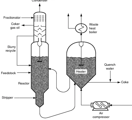
Figure 1-1. Schematic diagram of a fluid coke system (Speight, 2007). ... 4

Figure 1-2. Schematics of unwanted coke deposition (fouling) in the sheds and walls of the stripper section of a Fluid Coker (Adapted from Bi et al., 2005). ... 7

Figure 1-3. Mechanism of agglomerate formation (Bruhns and Werther, 2005). ... 8

Figure 1-4. Effect of liquid properties on the formation of agglomerates (McDougall et al., 2005). ... 9

Figure 1-5. Au198 decay graph (Moreira et al., 2010). ... 15

Figure 2-1. a) Fluidized bed apparatus components and instrumentation: Blower (1), air by-pass (2), orifice plate for flow measurement (3), wind box (4), air distributor (5), radioactive tracer-agglomerate (6), NaI scintillation sensors (7), USB hub (8), computer (9), 1.3 m of disengagement section (10), cyclone (11), fine powder collector recipient (12), shed (13). b) Schematic of the conical section of the fluidized bed with the single shed plus six layers of simulated foulant on top of it. ... 28

Figure 2-2. Schematic of the single shed structure with variable thicknesses of simulated foulant in the observation space. The height has a value of 8.5 cm divided in sections of 0.5 cm, which are 19 divisions... 29

Figure 2-3. An example of a calibration curve for detector 1. The X- axis presents the radiation in normalized data and the Y- axis presents the distance between the center of the detector and the tracer-agglomerate. As the particle is closer, the radiation is higher for that detector. ... 31

Figure 2-4. Schematics of a tracer-agglomerate motion to test accuracy of the RPT method (software and hardware) to determine its location (for clarity, only three detectors are

(15)

xiv

Figure 2-5. Typical RPT response for: a) X- at a constant 5 cm, b) Y- radius of 3cm, and c) Z- radius of 3cm plus 14 cm of height of the base; these graphs are plotted for the three coordinates in time in a non-stationary tracer environment... 34

Figure 2-6. Average standard deviation as a function of the tracer-agglomerate radiation. ... 34

Figure 2-7. Typical velocity arrow plot in the polar coordinates for the hydrodynamics behavior of the tracer particle when: (A) no shed is present, (B) shed is present, (C) shed plus maximum (3 cm) of foulant is present and (D) shed plus maximum (6 cm) of foulant is present. ... 35

Figure 2-8. Typical velocity arrow plot in the X coordinate for the hydrodynamic behavior of the tracer particle when: (a)No shed is present, (b) Shed is present, (c) Shed plus maximum (3cm) of foulant is present. (d) Shed plus maximum (6cm) of foulant is present. ... 36

Figure 2-9. Selected: a) Axial Segregation of the tracer particle along the fluidized bed; b) Accumulation of occurrences of the tracer particle along the fluidized bed. ... 37

Figure 2-10. a) Local occurrences of the tracer-agglomerate near the shed. b) Accumulation of occurrences of the tracer particle along the fluidized bed. ... 38

Figure 2-11. Calibration curve and trend line of the height of the foulant as a function of the standard deviation. ... 39

Figure 3-1. a) Blueprint of the new fluidized bed. b) New fluidized bed photo. ... 43

Figure 3-2. Sparger loop air feedstock. ... 45

Figure 3-3. Fluidized bed apparatus components and instrumentations: (1) Compressed air inlet; (2) orifice plates for flow measurement; (3) ball valves; (4) pinch valve; (5) elbow pressure taps for solids flow measurement; (6) 6.35 cm I.D. riser; (7) loop sparger; (8) three top-row sheds and two complete bottom-row shed plus two half; (9) 29.21 cm I.D.

disengagement zone; (10) cyclone; (11) γ-rays emitter; (12) twelve NaI Scintillation detectors

(16)

xv

Figure 3-4. a) Pressure taps along the fluidized bed. b) NI-DAQ and pressure transducers. . 47

Figure 3-5. a) Pressure tap to measure the flow of solids in the riser. b) Non-mechanical valve to divide the bed in two. ... 48

Figure 3-6. Screen shots of: a) the in-house software’s main windows, b) position rendition window and c) result analysis window. ... 49

Figure 3-7. Screenshot from: a) Complete Master/Slave System. b) The Slave computer screen. c) The Master computer screen... 51

Figure 3-8. Cold Flow Recirculating Fluidized Bed Measuring Zone. ... 52

Figure 3-9. Pyrolysis of Athabasca vacuum reside mix with gold. ... 56

Figure 3-10. Energy spectrum for: a) Epoxy/Gold agglomerate, b) Coke/Gold tracer-agglomerate. ... 56

Figure 3-11. Wet agglomerate behavior according to the model. ... 58

Figure 4-1. Simulated Agglomerate with: a) 1.94 mm diameter and a density of 1060 kg/m3. b) 12.65 mm diameter and a density of 1390 kg/m3. ... 67

Figure 4-2. Type of Interactions of the agglomerates with the sheds: a) Small cycle of the tracer-agglomerate in the measurement zone; b) Interaction from above the shed; c)

Interaction from below the shed; d) Crossing the shed zone interaction starting from below the shed; and e) crossing the shed zone interaction staring from above the shed. ... 69

Figure 4-3. Zones definitions to characterize the interactions of agglomerate with the shed: a) Measurement zones; b) Vicinity of the shed volume. ... 70

Figure 4-4. Average residence time per loop of the agglomerate inside the complete shed zone area (error bars represent the standard deviation). ... 71

(17)

xvi

Figure 4-6. Average residence time of the agglomerate below the shed zone (error bars

represent the standard deviation). ... 72

Figure 4-7. a) Typical mean Lagrangian velocity plot arrow for the X- and Z- coordinates. The X- coordinate is the coordinate that looks at the shed. b) Magnitude of the vertical component of the Lagrangian Velocity... 73

Figure 4-8. Typical frequency map of occurrences. ... 74

Figure 4-9. Change in velocity in the shed zone as a function of size and density. ... 74

Figure 4-10. Breakthrough velocities (error bars represent the standard deviation). ... 75

Figure 4-11. I) Velocity plot arrow for agglomerates: a) Tracer 1 ρ=1400 kg/m3 Ø_≈2.00 mm. b) Tracer 3 ρ=1060 kg/m3 Ø_≈2.00 mm. and c) Tracer 5 ρ=960 kg/m3 Ø_≈2.00 mm. II) Velocity plot arrow for agglomerates: a) Tracer 2 ρ=1400 kg/m3 Ø_≈13.00 mm. b) Tracer 4 ρ=1060 kg/m3 Ø_≈13.00 mm. and c) Tracer 6 ρ=890 kg/m3 Ø_≈13.00 mm. ... 76

Figure 4-12. Fraction of liquid entering the stripper lost to the burner for wet agglomerates (C0 = 30 wt%, for tracers 1 and 2) and semi-dry (C0 = 5 wt%, for tracers 3 and 4). ... 77

Figure 4-13. Fraction of liquid entering the stripper that reach the sheds level as vapor for wet agglomerates (C0 = 30 wt%, for tracers 1 and 2) and semi-dry (C0 = 5 wt%, for tracers 3 and 4). ... 77

Figure 5-1. Simulated Agglomerate with: a) 2.01 mm diameter and a density of 960 kg/m3. b) 12.65 mm diameter and density of 1400 kg/m3. ... 86

Figure 5-2. Zones definitions to characterize the interactions of agglomerate with the shed: a) Measurement zones. b) Vicinity of the shed area. ... 89

Figure 5-3. a) Residence time of the agglomerate in the shed zone as a function of the

(18)

xvii

shed as a function of the fluidization gas velocity. (With a 95% Confidence Interval, the error bars are very small to appear) ... 90

Figure 5-4. Residence time percentage of the agglomerate in the four distinctive of the fluidized bed plus the differential pressure of the shed zone as a function of the fluidization gas velocity. ... 91

Figure 5-5. Velocity plot arrow in the shed zone as a function of the fluidization gas velocity. ... 91

Figure 5-6. a) Residence time of the agglomerate in the shed zone as a function of the solid recirculation rate. b) Residence time of the agglomerate in the vicinity of the shed as a function of the solid recirculation rate. c) Residence time of the agglomerate below shed as a function of the solid recirculation rate. And, d) Residence time of the agglomerate above the shed zone as a function of the fluidization gas velocity. (With a 95% Confidence Interval, the error bars are very small to appear) ... 92

Figure 5-7. Percentage of time of the agglomerate in the four distinctive of the fluidized bed plus the differential pressure of the shed zone as a function of the solid recirculation rate. .. 93

Figure 5-8. Velocity plot arrow in the shed zone as a function of the solid recirculation rate. ... 94

Figure 5-9. Velocity plot arrow for polar coordinates in the entire measurement zone. ... 94

Figure 5-10. a) Residence time of the agglomerate in the shed zone as a function of the percentage of beads. b) Residence time of the agglomerate in the vicinity of the shed as a function of the percentage of beads. c) Residence time of the agglomerate below shed as a function of the percentage of beads rate. And, d) Residence time of the agglomerate above shed as a function of the fluidization gas velocity. (With a 95% Confidence Interval, the error bars are very small to appear) ... 95

(19)

xviii

Figure 5-12. a) Velocity plot arrow in the shed zone for dense agglomerate as a function of the beads in the bed. b) Velocity plot arrow in the shed zone for light agglomerate as a function of the beads in the bed. ... 97

Figure 5-13. Fraction of liquid entering the stripper that reaches the sheds level as vapor for: a) wet agglomerates; and, b) dry agglomerates. (With a 95% Confidence Interval, the error bars are very small to appear) ... 98

Figure 6-1. Simulated Agglomerate with: a) 1.94 mm diameter and a density of 1060 kg/m3. b) 12.65 mm diameter and a density of 1390 kg/m3. ... 105

Figure 6-2. Types of sheds tested: a) No shed; b) Normal sheds; c) Mesh-Shed and d) Mega-Sheds. ... 107

Figure 6-3. Normal-shed configuration with a: a) Small, b) Normal and c) Big, Cross Section Area Reduction. ... 107

Figure 6-4. Zones definitions to characterize the interaction of agglomerate with the sheds. ... 109

Figure 6-5. a) Average residence time of the agglomerate above the shed level as a function of agglomerate density; b) Average residence time of the agglomerate in the shed zone as a function of agglomerate density; and c) Average residence time of the agglomerate below the shed level as a function of agglomerate density. (With a 95% confidence interval, the error bars are very small to appear). ... 110

Figure 6-6. Fraction of liquid entering the stripper that reaches the sheds level as vapor for wet (C0 = 30 wt%, for tracers 1 and 2) and semi dry (C0 = 5 wt%, for tracers 3 and 4) agglomerates. This for: a) when sheds are located inside the bed; and b) when no internals are present. (The error bars represent the data with a 95% confidence interval) ... 111

(20)

xix

Figure 6-8. a) Upward velocities as a function of agglomerate densities, and b) Downward velocities for as a function of agglomerate densities. (With a 95% confidence interval, the

error bars are very small to appear). ... 112

Figure 6-9. Velocity plot arrow in the shed zone as a function of agglomerate density for: a) small agglomerate (Ø ≈ 2) and b) big agglomerate (Ø ≈ 13). ... 113

Figure 6-10. Differential pressure of the shed zone as a function of the shed type. (The error bars represent the data with a 95% confidence interval). ... 114

Figure 6-11. Average residence time of the agglomerate above the shed, in the shed, below the shed zones as a function of the shed type. (The error bars represent the data with a 95% confidence interval). ... 115

Figure 6-12. a) Fraction of liquid entering the stripper that reaches the sheds level as vapor as a function of shed type for wet agglomerate (C0 = 30 wt%, for tracer 2). b) Fraction of liquid entering the stripper lost to the burner as a function of shed type (C0 = 30 wt%, for tracer 2). (The error bars represent the data with a 95% confidence interval) ... 115

Figure 6-13. Percentage of liquid entering the stripper that reaches the shed as vapor as a function of the percentage of liquid entering the stripper lost to the burner, for each of the different internals. ... 116

Figure 6-14. Upward and downward velocities as a function of the shed type. ... 117

Figure 6-15. Velocity plot arrow in the shed zone as a function of the type of shed. ... 118

Figure 6-16. Frequency map of occurrences as a function of the type of shed. ... 119

Figure 6-17. Differential pressure of the shed zone as a function of the bed open area. (With a 95% confidence interval, the error bars are very small to appear). ... 120

(21)

xx

Figure 6-19. a) Fraction of liquid entering the stripper that reaches the sheds level as vapor as a function of the bed open area (C0 = 30 wt%, for tracers 7). b) Fraction of liquid entering the stripper lost to the burner as a function of the bed open area (C0 = 30 wt%, for tracers 7).

(The error bars represent the data with a 95% confidence interval) ... 121

Figure 6-20. Upward and Downward breakthrough velocities as a function of the bed open area. ... 121

Figure 6-21. Velocity plot arrow in the shed zone as a function of the bed open area. ... 122

Figure 7-1. Simulated Agglomerate with 12.65 mm diameter. ... 129

Figure 7-2. Voltesso injection system. ... 131

Figure 7-3. Zones definitions to characterize the interaction of agglomerate with the sheds. ... 132

Figure 7-4. Differential pressure of the shed zone as a function of the amount of liquid inside the bed using: a) tracer 2; and b) tracer 1 (With a 95% confidence interval, the error bars are too small to appear) ... 133

Figure 7-5. Residence time in the above the shed, in the shed and below the shed zone as a function of the amount of liquid inside the bed using tracer 1 (With a 95% confidence interval, the error bars are too small to appear). ... 133

Figure 7-6. Residence times above the shed, in the shed zone and below the shed as a function of the amount of liquid inside the bed using tracer 2 (With a 95% confidence interval, the error bars are too small to appear). ... 134

Figure 7-7. Fraction of liquid entering the stripper that reaches the sheds level as vapor for semi-dry and wet agglomerates as a function of the amount of liquid inside the bed (With a 95% confidence interval, the error bars are very small to appear). ... 135

(22)

xxi

Figure 7-9. Avalanche time as a function of the percentage of liquid in the bed. ... 137

Figure 7-10. Residence time in the above the shed, in the shed and below the shed zone as well as differential pressure as a function of the amount of coke inside the bed using tracer 1 (With a 95% confidence interval, the error bars are very small to appear). ... 138

Figure 7-11. Fraction of liquid entering the stripper and reaches the sheds level as vapor for wet agglomerates as a function of the amount of coke inside the bed (With a 95% confidence interval, the error bars are very small to appear). ... 139

Figure 7-12. Fraction of liquid entering the stripper lost to the burner for wet agglomerates as a function of the amount of coke inside the bed (With a 95% confidence interval, the error bars are very small to appear). ... 140

Figure 7-13. Lagrangian velocity vector plot. ... 141

Figure 8-1. Schematics of ring baffle (Wyatt et al., 2011). ... 146

Figure 8-2. Simulated Agglomerate with 12.65 mm diameter. ... 148

Figure 8-3. Baffle dimensions and characteristics. ... 149

Figure 8-4. Frequency map of occurrences. ... 150

Figure 8-5. Flux tubes. ... 150

Figure 8-6. Zones definitions to characterize the interaction of agglomerate with the baffles. ... 151

Figure 8-7. Residence time above the baffle zone, in the baffle zone and below the baffle zone of the big agglomerate as a function of the baffle angle (Vg = 0.24 m/s) ... 152

Figure 8-8. Fraction of the ratio of residence time with baffle divided by the residence time without internals as a function of the baffle angle (Vg = 0.24 m/s) ... 153

(23)

xxii

Figure 8-10. Fraction of liquid entering the stripper lost to the burner as a function of the baffle angle (Vg = 0.24 m/s) ... 154

Figure 8-11. Average time it takes a wet agglomerate to enter the baffle zone once it enters the measuring zone as a function of the baffle angle (Vg = 0.24 m/s) ... 155

Figure 8-12. Average Lagrangian velocity plot arrows in polar coordinates for baffles, shed and no internals (Vg = 0.24 m/s) ... 155

Figure 8-13. Time to first pass for all the baffles with (only flat to the bottom) and without flux tubes, as well as with and without sheds as a function of the fluidization gas velocity (for baffles with flux tubes, the flux tube length was 2.90 cm for the 45° angle baffle and 5.11 cm for a 30° angle baffle). ... 157

Figure 8-14. Ratio of time to first pass for a baffle with flux tubes to the time to first pass for a baffle without flux tubes, as a function of the fluidization gas velocity (Flux tube length of 2.70 cm for the 45° angle baffle and 4.91 cm for a 30° angle baffle) ... 157

(24)

xxiii

List of Appendices

Appendix A: RPT Single Computer Software Code ... 166

Appendix B: RPT Master Computer Software Code ... 216

Appendix C: RPT Slave Computer Software Code ... 223

Appendix D: Matlab Presentation Software Code ... 231

Appendix E: Drying Model Equation ... 236

Appendix F: John Wiley and Sons License Terms and Conditions ... 239

(25)

xxiv

Nomenclature

A Strength of the radiation source SD Square root of the mean sum of square differences

a Coefficient of the polynomial Regression

ST Sampling time (t)

b Coefficient of the polynomial

Regression StD Critical defluidization Stoke number

C Counts Stv Stoke number

C0 Initial liquid concentration Stv* Minimum Stoke number

Cp Heat capacity (J/K) T Temperature (°C)

CSum Summation of the counts from all

twelve detectors t Time (s)

c Coefficient of the polynomial Regression

tc Time for full conversion (s)

ci Counts for ith detector uo Granule collisional velocity (m/s)

e Particle coefficient or restitution U Superficial gas velocity (m/s)

Fs Flow of solids (kg/s) Um Minimum modify fluidization velocity (m/s)

Fv Mass flowrate of vapor (kg/s) Ur Gas velocity in the riser. (m/s)

F Oscillation frequency Us Amplitude of oscillation (m/s)

h Binder thickness (µm) v γ-rays per disintegration

hFouling Height of foulant in the shed (cm) XShed Occurrences at a certain height

ho Length of asperities (µm) XFouling Occurrences at a certain height register for the shed plus fouling k Thermal conductivity of coke layers

W/(m·K)

x Coordinate x from the tracer particle (m)

m Mass (kg) xi Coordinate x from the detector i

(m) mL Mass of liquid in the agglomerate at

time t (m/s)

y Coordinate y from the tracer particle (m)

mL0 Initial mass of liquid in the

agglomerate at t = 0 (m/s) yc Coke yield

R Particle Radius (m) yi Coordinate y from the detector i (m)

r Distance between detectors and

tracer particle (m) z Coordinate z from the tracer particle (m)

(26)

xxv

Greek Letters

α Unknown constant ∆HLiq Enthalpy change when the liquid

reacts (J/kg)

γ Constant φ Photopeak ratio

ε Total efficiency η Normalize radial position

µ viscosity (kg/m·s) Ø Diameter (mm)

ρ Density (kg/m3) ΦD Rate of deposition (kg/s)

∆P Pressure drop in the elbow (Pa) ΦR Rate of removal (kg/s)

∆H Enthalpy change (J/kg) Ψi Relative counts for a particular

(27)

xxvi

Preface

The thesis was written in an integrated article format, with six articles in total, and three extra sections were added:

1. Introduction (Chapter 1): Literature review of bitumen; the Fluid CokerTM, specifically the stripper section; the Radioactive Particle Tracking technique; and finally the objectives of the research.

2. Equipment and Software Design (Chapter 3): The design and construction of the experimental unit; development of the software and mathematical tools that were used to analyze the data; and finally the construction of the simulated agglomerates. 3. Conclusion and Recommendations (Chapter 9): General conclusions of the research

and recommendations for future work in the unit or the potential use of the Radioactive Particle Tracking technique.

The order of the Chapters 2 to 8 reflects when the experiment or the construction was made; i.e. the experimental work described in Chapter 2 (Application of Radioactive Particle Tracking to Indicate Shed Fouling in the Stripper Section of a Fluid Coker) was performed before the Cold Flow Recirculating Fluidized Bed was completed (Chapter 3). The six integrated articles are:

1. Application of Radioactive Particle Tracking to Indicate Shed Fouling in the Stripper Section of a Fluid Coker (Chapter 2). The license for publication in this thesis is presented in Appendix F.

2. Agglomerate Behavior in Recirculating Fluidized Bed with Sheds: Effect of Agglomerate Properties (Chapter 4)

3. Agglomerate Behavior in Recirculating Fluidized Bed with Sheds: Effect of Bed Properties (Chapter 5)

4. Agglomerate Behavior in Recirculating Fluidized Bed with Sheds: Effect of the Sheds (Chapter 6)

5. Agglomerate Behavior in Recirculating Fluidized Bed with Sheds: Effect of Voltesso and Amount of Fluidized Material (Chapter 7)

(28)

xxvii

If you take a look at science in its everyday function, of course you find that scientists run the

gamut of human emotions and personalities and character and so on. But there’s one thing

that is really striking to the outsider, and that is the gauntlet of criticism that is considered

acceptable or even desirable. The poor graduate student at his or her Ph.D. oral exam is

subjected to a withering crossfire of questions that sometimes seem hostile or contemptuous;

this from the professors who have the candidate’s future in their grasp. The students

naturally are nervous; who wouldn’t be? True, they’ve prepared for it for years. But they

understand that at that critical moment they really have to be able to answer questions. So in

preparing to defend their theses, they must anticipate questions; they have to think, “Where

in my thesis is there a weakness that someone else might find—because I sure better find it

before they do, because if they find it and I’m not prepared, I’m in deep trouble”.

(29)

Chapter 1

1 INTRODUCTION

The research presented in this dissertation addresses the behavior of simulated agglomerates and their interactions with the internals of the stripping section of Fluid CokersTM that are called sheds. A key motivation for this research is to understand the hydrodynamics of the agglomerates and why they foul internals. Extensive fouling impairs stripping and may cause the premature shutdown of the reactor. This chapter presents a brief introduction of bitumen, Fluid Coking, agglomerates and the Radioactive Particle Tracking (RPT) technique. Finally, it introduces the objectives of this research.

1.1 Fouling

One of the most persistent problems encountered in Fluid CokingTM is the fouling of the stripper section of the reactor by solid coke deposits. The accumulation of unwanted material on the surfaces of process equipment is usually referred to as fouling. The rate of fouling [Equation (1.1), where m is mass and t is time] can be defined by the difference between the rate of deposition (ΦD) and the rate of removal (ΦR). When

fouling occurs in a process, two possible scenarios can occur:

1. The rate of deposition is always greater than the rate of removal, and in time, a complete obstruction to the flow is formed.

2. At certain point in time, the rate of removal is equal to the rate of deposition and equilibrium is reached (Bott, 1995).

_D _R

t m

φ

φ −

= ∂ ∂

(1.1)

(30)

1.2 Bitumen

With the quality of crude oil diminishing all around the world, the lowest quality crude oils rich in sulfur, metals and fractions that boil above 560°C are becoming more important to the petrochemical industry (Hammond et al., 1997).

Bitumen is a naturally occurring product that is found in deposits where there is little permeability. Oil sand bitumen is a high-boiling material with little material that boils below 350 °C. Oil sands have been described in the United States (FE-76-4) as:

“…the several rock types that contain an extremely viscous hydrocarbon which is not

recoverable in its natural state by conventional oil well production methods including

currently used enhanced recovery techniques. The hydrocarbon-bearing rocks are

variously known as bitumen-rocks oil, impregnated rocks, oil sands and rock asphalt”

(Speight, 2007).

Oil sands are a mixture of sand, bitumen, mineral-rich clays and water. The bitumen content of the mined oil sands is about 10 – 12 wt% depending upon the location. When compared to conventional crude oils, bitumen is a thick material that has higher concentrations of high molecular weight species and heteroatomic species such as nitrogen, sulfur and metals (Soundararajan, 2001).

The oils sands in the Athabasca region of Alberta, Canada, are first mined. The bitumen is then extracted in two steps. First, the oil sands are washed with hot water to remove most of the sand and clay. This results in a sticky froth containing large volumes of water and solids. In the second step, the froth is diluted with a light hydrocarbon to cause the water and solids to settle out quickly, yielding diluted bitumen with only traces of water and solids. The light hydrocarbons are boiled off and bitumen is obtained. In an alternate, in-situ, process, called Steam Assisted Gravity Drainage (SAGD), steam is injected underground to heat the bitumen, thus reducing its viscosity and allowing it to drain into a lower well, from which it can be pumped out.

(31)

fraction is then routed to a vacuum distillation unit where reduced pressure is used to achieve further separation without thermal cracking. The temperature limit for conventional distillation is an atmospheric boiling point of 524-540 °C, which corresponds to a temperature of 250 °C in a typical vacuum system. In the vacuum distillation unit, the atmospheric tower residue is separated into vacuum gas oil, lubricating oil and vacuum residue fractions. The residue from the atmospheric tower is vacuum distilled for two reasons. First, vacuum distillation helps remove volatile materials and recover a higher fraction of product hydrocarbons. Secondly, removing the volatiles prevents them from being lost to gas through over-cracking in downstream refining operations (Soundararajan, 2001).

The enormous resources of oil sands bitumen in Western Canada require extensive processing in order to produce transportation fuels (gasoline, diesel, etc.), particularly the vacuum residue fraction which makes up to 50-60 wt % of the hydrocarbons in the oil sands. Coking is one of the most important technologies for processing the vacuum residue, which is converted to permanent gases, valuable distillable products and solid coke residues (Gray et al., 2003).

1.3 Coking

Coking is a thermal process for the continuous conversion of heavy hydrocarbons into synthetic crude oil plus coke and permanent gases as by-products. Several processes have been used to thermally crack bituminous materials (Speight, 2007):

• Visbreaking: Short for Viscosity Breaking. This process was developed to reduce the viscosity of highly viscous hydrocarbons by introducing the product into a furnace in order to achieve “mild” thermal cracking and thus meet fuel oil specifications.

• Delayed Coking: Semi-continuous process in which vacuum residues are

heated and then introduced into a coking drum, which provides very long residence times that enable more severe thermal cracking.

(32)

products. This process decreases the yield o greater quantities of more valuable liquid products.

• FlexicokingTM

gasification unit where excess coke is gasified.

1.3.1 Fluid Coking

Fluid Coking is a process for

thermal cracking into lighter hydrocarbon products. The heavy feed is preheated to 350 °C and injected through steam

500 °C to 550 °C. The bed temperature must be at a moderate level to avoid over

2004).

Figure 1-1. Schematic diagram of a fluid coke system (Speight, 2007).

The feedstock is injected in a downward it heats up and cracks into smaller

the particles flow down to a stripper where valuable oil vapors trapped between the c particles are recovered through steam stripping. The stripper section of the Coker consists of a system of baffles (sheds) that enhance the removal of hydrocarbon vapors

products. This process decreases the yield of undesirable coke and produces greater quantities of more valuable liquid products.

TM_{: A process that is very similar to Fluid Coking, but includes a} gasification unit where excess coke is gasified.

Fluid Coking

is a process for refining heavy hydrocarbon bitumen through thermal cracking into lighter hydrocarbon products. The heavy feed is preheated to C and injected through steam atomization spray nozzles into a fluidized bed at °C to 550 °C. The bed temperature must be high enough to achieve cracking but kept at a moderate level to avoid over-cracking to low value permanent gases (House et al.,

Schematic diagram of a fluid coke system (Speight, 2007).

The feedstock is injected in a downward-flowing bed of hot coke particles, where up and cracks into smaller vapor molecules. Vapors rise through the bed while the particles flow down to a stripper where valuable oil vapors trapped between the c particles are recovered through steam stripping. The stripper section of the Coker consists of a system of baffles (sheds) that enhance the removal of hydrocarbon vapors

f undesirable coke and produces

: A process that is very similar to Fluid Coking, but includes a

refining heavy hydrocarbon bitumen through thermal cracking into lighter hydrocarbon products. The heavy feed is preheated to atomization spray nozzles into a fluidized bed at high enough to achieve cracking but kept cracking to low value permanent gases (House et al.,

(33)

from the fluidized coke particles. The down-flowing coke particles are then conveyed to a burner where they are reheated through partial combustion and hot coke particles are recirculated back to the reactor where they provide the heat required for the endothermic thermal cracking process, as described in Figure 1-1. Excess coke particles are removed, quenched and stockpiled.

When sprayed into the fluidized bed, the hydrocarbon feed is dispersed into very fine droplets in a wide spray, which significantly increases the phase contact area, in the reactor in order to provide a proper cracking environment for the bitumen feed, without major heat and mass transfer limitations. The evenly distributed droplets enhance the heat transfer, which is desirable, for a rapid and effective process (Base et al., 1999). The liquid-solid contact for this process is measured by the amount and quality of the product yields, the reactor operability and finally the process efficiency (House et al., 2004).

Gray et al. (2003) reported that the time required for Athabasca bitumen to react and lose its adhesion or ability to form stable liquid bridges between particles, thus form agglomerates is around 24 s at 503 °C. In addition, the adhesive forces due to the reacting material are significant only when the film was still liquid and able to form liquid bridges between particles. Coke particle growth can occur by two mechanisms:

1. Normal growth by virtue of product coke laid down on the individual particles.

2. By agglomeration of coke-particles.

(34)

1.3.2 Sheds

In some fluidized beds, especially with Group B powders (Geldart, 1973), internals are used in order to improve the fluidization by breaking and re-distributing the bubbles (Issangya et al., 2008). Bubble size is very important for gas/solid mass transfer in bubbling fluidized beds. The gas from inside the bubbles comes in contact with the coke particles in the clouds around the bubbles. This mass transfer between gas and solid is improved by reducing the bubble size and renewing the bubble surroundings by interchanging the gas component from the bubbles with that from the emulsion phase (Yang, 2003).

Horizontal baffles have been used to eliminate gas bypassing in deep fluidized beds of Geldart A powders, i.e. Fluid Catalytic Cracking (FCC) (Issangya et al., 2008; Issangya et al., 2013). Moreover the ability of baffles to reduce the gas bypassing is dependent on the vertical baffle spacing, effective open area and the spacing of the internals in the fluidized bed (Issangya et al., 2007). Rings, inverse cones and bluff bodies internals have been studied in the riser of Circulating Fluidized Beds (CFB) and are said to improve the radial solid distribution and improve gas-solids mixing (Jiang et al., 1991; Zhu et al., 1997). Hartholt et al. (1997) have shown that perforated plates located in the middle of a fluidized bed promote particle segregation by size while reducing the bubble size (Yang, 2003).

Luckenbach (1969) was the first one to patent and use shed decks in a fluid catalytic cracking reactor. Later, Blaser et al. (1986) patented the use of shed decks in the stripping section of a Fluid Coker.

(35)

Figure 1-2. Schematics of unwanted coke deposition (fouling) in the sheds and walls of

the stripper section of a Fluid Coker

1.4 Agglomerates

The agglomeration of solids occurs in many fluidization processes. In the pharmaceutical and fertilizer industries, agglomeration is something that is desirable and is used to reduce process problems like dustiness (Weber et al., 2009). In thermal cracking processes such as

production yield (agglomerates leave the Coker valuable un-cracked hydrocarbons, only to be burn

the reactors internals and surfaces. Fouling of the sheds in the stripper section leads to the premature shutdown of the unit.

1.4.1 Agglomerate Formation

Bruhns and Werther

formation based on experimental research; as the injected liquid is introduced into the fluidized bed not all the liquid is instantaneously vaporized (although the bed is oper above the boiling point of the liquid). Particles are suck

Schematics of unwanted coke deposition (fouling) in the sheds and walls of of a Fluid Coker (Adapted from Bi et al., 2005).

Agglomerates

The agglomeration of solids occurs in many fluidization processes. In the pharmaceutical and fertilizer industries, agglomeration is something that is desirable and is used to reduce process problems like dustiness (Weber et al., 2009). In thermal such as coking, agglomeration is not desirable because it affects production yield (agglomerates leave the CokerTM with a considerable amount of highly cracked hydrocarbons, only to be burned in the burner) and creates fouling of reactors internals and surfaces. Fouling of the sheds in the stripper section leads to the premature shutdown of the unit.

Agglomerate Formation

Bruhns and Werther (2005) proposed a model (Figure 1-3) of agglomerate on experimental research; as the injected liquid is introduced into the fluidized bed not all the liquid is instantaneously vaporized (although the bed is oper above the boiling point of the liquid). Particles are sucked into the liquid jet and

Schematics of unwanted coke deposition (fouling) in the sheds and walls of

The agglomeration of solids occurs in many fluidization processes. In the pharmaceutical and fertilizer industries, agglomeration is something that is desirable and is used to reduce process problems like dustiness (Weber et al., 2009). In thermal coking, agglomeration is not desirable because it affects amount of highly in the burner) and creates fouling of reactors internals and surfaces. Fouling of the sheds in the stripper section leads to the

(36)

immediately form agglomerates. These agglomerates then are transported into the rest of the fluidized bed.

Figure 1-3. Mechanism of agglomerate formation (Bruhns and Werther, 2005).

Ariyapadi et al. (2003) studied the agglomerate formation mechanism by using X ray imaging while injecting a radio opaque liquid tracer mixed with ethanol in order to visualize the jet cavity. Agglomerates appeared to form via coalescence of droplets and particles at the end of the jet cavity.

1.4.2 Effect of Liquid Properties

Schafer and Mathiesen

the formation of agglomerates. The research identified two mechanisms through which the initial wetting of the liqu

1. For small droplets: Wetting occurs through the distribution of droplets on individual solid particles. The

occurs.

2. For large droplets: The immersed inside the liquid.

immediately form agglomerates. These agglomerates then are transported into the rest of

Mechanism of agglomerate formation (Bruhns and Werther, 2005).

Ariyapadi et al. (2003) studied the agglomerate formation mechanism by using X ray imaging while injecting a radio opaque liquid tracer mixed with ethanol in order to

ity. Agglomerates appeared to form via coalescence of droplets and particles at the end of the jet cavity.

Effect of Liquid Properties

Schafer and Mathiesen (1996) used a shear mixer to study the effect

the formation of agglomerates. The research identified two mechanisms through which the initial wetting of the liquid droplets and particles occur:

For small droplets: Wetting occurs through the distribution of droplets on individual solid particles. Thereafter, coalescence between wet particles

For large droplets: The wetting involves a large number of particles be immersed inside the liquid.

immediately form agglomerates. These agglomerates then are transported into the rest of

Mechanism of agglomerate formation (Bruhns and Werther, 2005).

Ariyapadi et al. (2003) studied the agglomerate formation mechanism by using X-ray imaging while injecting a radio opaque liquid tracer mixed with ethanol in order to

ity. Agglomerates appeared to form via coalescence of droplets and

1996) used a shear mixer to study the effect of viscosity on the formation of agglomerates. The research identified two mechanisms through which

For small droplets: Wetting occurs through the distribution of droplets on after, coalescence between wet particles

(37)

Because of the results of open air experiments in which the Sauter mean diameter of the liquid droplets is equivalent to the Sauter mean diameter of the coke particles, the first mechanism is believe to be happening inside Fluid CokersTM (House, 2007).

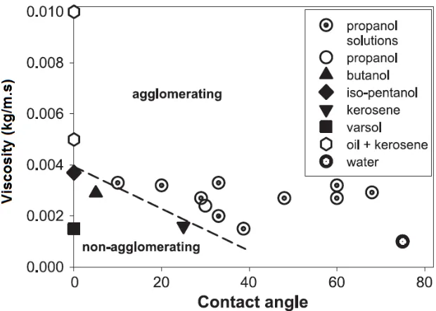
McDougall et al. (2005) studied the liquid properties that affect the formation of agglomerates inside fluidized beds when liquid is sprayed in. The research reported that the viscosity of the liquid and contact angle are the most important variables in the formation of agglomerates independently of the fluidization gas velocity. The formation of agglomerates with liquid that wets well the 135 µm particles (low contact angle

between the liquid and the solid surface) occurs only when the liquid has a high viscosity. For liquids that do not wet well particles (high contact angle), there is always the formation of agglomerates as presented in Figure 1-4.

Figure 1-4. Effect of liquid properties on the formation of agglomerates (McDougall et al., 2005).

1.4.3 Granulation

(38)

In their work on agglomerates fragmentation, Salman et al. (2004) presented different failure modes of agglomerates breakage as a function of the impact velocity. Larger and porous agglomerates promote the chipping (localised damage) of the agglomerate. Moreover Salman et al. (2003) concluded that the probability of agglomerate fragmentation is dependent upon size, material and impact velocity. Finally Subero and Ghadiri (2001) determined that there are two main types of breakage, localized damage and distributed damage. These findings are in accordance with results from Weber et al. (2006): at low fluidization gas velocities, erosion predominates and fragmentation prevails at high fluidization gas velocities.

Weber et al. (2009) showed that when erosion is the dominant mechanism of destruction, bigger and denser agglomerates are more stable than smaller and lighter ones. In addition, and up to 3 cP viscosity, an increase in liquid viscosity makes the agglomerates more stable (they can survive the harsh environment inside fluidized beds, something that is not desirable for Fluid CokersTM). Weber et al. (2006) concluded that the most stable agglomerates are formed with small spherical particles that are completely wetted by liquid. This is in accordance with findings from Dunlop et al. (1958), who found that particles larger than 70 µm adhere to each other because of liquid coating will be pulled apart because of fluidized bed forces, at the same time particles below 70 µm stay together to form an agglomerate.

Because the fouling in the stripper section is closely related to particle agglomeration, further study of the mechanism that leads to the coalescence between coke particles by liquid bitumen is needed. Granulation theory has been used in the past to study the mechanism that leads to fouling.

Ennis et al. (1991) proposed a minimum Stokes number [Stv*, Equation (1.2)] above which colliding granules rebound, which avoids agglomerate formation.

(1 )ln( )

0 *

h h e

(39)

Where:

• e is the particle coefficient of restitution.

• ho is the length of asperities on particle surface.

• h is the binder layer thickness.

By comparing Stokes number, Equation (1.3), with the minimum Stokes number [obtained from Equation (1.2)], Ennis et al. (1991) came up with a classification of the coalescence phenomena. When particles with initial Stokes number less than the critical value collide (Stv < Stv*), they coalesce. Collisions of particles with higher Stokes number (Stv > Stv*), result in a rebound of the colliding particles.

µ ρ

9 8 u₀R

St_v = _(1.3)

Where:

• ρ is the particle density.

• uo initial relative granule collisional velocity.

• R particle radius

• µ is the binder viscosity.

Equations (1.2) and (1.3) can be used to analyze defluidization in fluidized bed granulation. The addition of a binder to the fluidized bed increases the minimum fluidization velocity due to changes in the porosity of the fluidized medium. The liquid bridges generated by the binder have a tendency to increase the porosity of the bed, thus this increases the velocity of the gas, and results in a pressure drop equal to the weight of the bed, for example, the minimum fluidization condition. Therefore, the critical defluidization Stokes number [Equation (1.4)] is:

(1 1)ln( )

9 ) ( 8 0 0 * h h e R U U St m

D = +

− = µ ρα (1.4) Where:

(40)

• Um is the modified minimum fluidization velocity due to viscous layers.

• Uo is the minimum initial fluidization velocity.

Gray (2002) analyzed the work done by Ennis et al. (1991) in relation to the context of Fluid Coking. Solving for the minimum fluidization velocity [Equation (1.5)] suggests that this velocity increases in proportion to the logarithm of the liquid film thickness:

ln( )

8 ) 1 1 ( 9

0 0

h h R

e U

U_m

ρα

µ +

+

= (1.5)

The film thickness is directly controlled by the rate of liquid feeding into a fluidized bed with a given amount of particles. The reaction and mass transfer processes favor minimal values of h, and this relationship suggests simultaneous benefits for thin films in avoiding defluidization. Optimizing process variables such as feed atomization, the number, position and orientation of jets or nozzles for the liquid feed, gas flow rate, and the reactor length to diameter ratio may help to achieve thinner films. In addition, Equation (1.5) suggests that the larger the particle, the smaller the increase in minimum fluidization velocity due to the presence of liquid binder. The overall conclusion can be summarized as: thinner films, larger particles and rougher particles help reduce the rate of particle adhesion. Moreover, the increase in the local characteristic velocity, Uo, increases the Stokes number near the reactor internal surfaces and helps avoid falling below the critical Stokes number and thus mitigates fouling.

(41)

fluidizing medium is effective to promote dispersion. The larger particles are fluidized easily and generate impaction and attrition forces that act as a dispersion forces on the adhesive particles (Masuda et al., 2006)

Parveen et al. (2013) presented a novel way to detect fragmentation of agglomerates inside a fluidized bed by using Radio Frequency Identification (RFID). The research concluded that the stability of an agglomerate is a function of its liquid content, its bulk density and the size of its constituent particles. An increase of the liquid content or bulk density increase the agglomerate stability, while larger constituent particles will make the agglomerate less stable. Also concluded that the average survival time for an agglomerate inside the bed is directly proportional to the critical shear force that is needed to break the agglomerate. The superficial gas velocity plays an integral role in determining which mechanism, erosion or fragmentation, cause agglomerate destruction: erosion predominates at low velocities and fragmentation at high velocities. When the superficial gas velocity is sufficiently high, fragmentation predominates, all agglomerates are fractured and no type of agglomerate is able to survive in a fluidized bed (Weber et al., 2006).

Wang and Rhodes (2005) presented a way to increase the velocity of the fluidized bed without affecting the overall operation of the bed. A major constraint associated with an increase in gas velocity is that the rate of particle elutriation may significantly increase. This is particularly true when the bed consists of particles with a wide size distribution. To take advantage of the effect of higher fluidization velocity without incurring excessive particle elutriation, a higher fluidization velocity is intermittently applied without increasing the time-averaged superficial gas velocity; such as applying gas-phase pulsation in the form of Equation (1.6).

U(t)=U₀+U_ssin(2πft) (1.6)

Where:

• U is superficial gas velocity.

(42)

• Uo time-averaged superficial gas velocity.

• Us amplitude of oscillation.

In practice, Us is set to be considerably smaller than Uo so that the oscillation component makes up only a small fraction of the total gas flow; with this approach, elutriation should not be impacted. Also, it has been reported that the effect of pulsation is most pronounced when the frequency of imposed pulsation matches the natural frequency of the bed.

1.5 Radioactive Particle Tracking

The Radioactive Particle Tracking (RPT) technique applied to fluidized beds consists of detecting the amount of radiation in the form of γ-rays, emitted by a single

radioactive tracer-particle (Because the focus of this research is related to agglomerates, the radioactive tracer-particle term, which is used in most RPT publications, will be changed to radioactive tracer-agglomerate in this work). The detected radiation is a function of distance from an array of gamma ray detectors located externally to the bed. The main advantage of this method is its non-intrusive nature; data can thus be obtained without disrupting the gas-solid flow inside the vessel.

A complete RPT system includes:

• A single radioactive tracer-agglomerate emitting γ-rays.

• Several scintillation detectors to sense the radiation emitted by the tracer-agglomerate.

• One computer or computers to record, process, and analyze the data from each detector.

(43)

polyurethane to match the diameter and density to that of the bed particles. Chaouki et al. (1997) described other attempts to introduce material that can be irradiated to produce a radioactive tracer. Regardless of the method or tracer preparation and the materials used, all suffer from similar limitations, i.e. the material is not exactly the same as the fluidized medium.

Radioactive gold (Au198), is preferred for RPT experiments because it decays very fast (as presented in Figure 1-5) and it decays into a stable isotope of Mercury (Hg198), which is very desirable for health concerns (Moreira et al., 2010).

Figure 1-5. Au198 decay graph (Moreira et al., 2010).

(44)

There are several position rendition techniques that can be used to determine the x-, y-, and z- coordinates of the tracer-agglomerate inside the reactor as a function of time using the radiation signal obtained from the scintillation detectors. The Computer Automated Radioactive Particle Tracking (CARPT) and the Monte Carlo simulation methods are the two most common ones.

1.5.1 CARPT Rendition Technique

The CARPT method was originally developed by Lin et al. (1985). The main outcome of this method is that the number of γ-rays counted by a detector depends

unequivocally on the distance between the tracer-agglomerate position and a virtual center in the detector surface. Once this virtual center is determined, a calibration curve relating γ-rays counts to distance is established for each detector for a condition identical

to those of the particle tracking. The calibration data obtained is expressed in a functional form using a curve fit of the raw data. Polynomial fits with various orders are used in order to describe the different domains of distance versus γ-rays counts relationships

(Chaouki et al., 1997).

By defining an arbitrary reference frame and denoting by (x,y,z) the unknown coordinates of the tracer as well as the coordinates of the virtual center of ith detector (xi, yi, zi), then for each detector the formula can be written as shown in Equation (1.7):

2 2 2 2

) ( ) ( )

( i i i

i x x y y z z

r = − + − + − (1.7)

Where r is the distance obtained from the polynomial fitting. The availability of distance measurements from many scintillation detectors results in data redundancy for location determination. To take advantage of this planned redundancy, a weighted least-square method based on an exact linearization scheme is used to obtain the tracer position (Lin et al., 1985).

(45)

between the tracer and a horizontal plane through the virtual center of the scintillation detector.

1.5.2 Monte Carlo Rendition Technique

In order to avoid extensive in-situ calibration, Professor Chaouki and his group at École Polytechnique de Montréal developed a phenomenological approach to account for geometry and radiation effects in RPT. With their rendition technique, the determination of the tracer position from the detectors counts requires the construction of a map of counts as a function of the possible coordinates of the particle by using Equation (1.8). Since a certain fraction of the γ-rays are absorbed by the fluidized material and by the

vessel walls, a new map is needed whenever the density of the medium to be studied changes (Chaouki et al., 1997).

ϕε τ

ϕε

A vA ST C

+ =

1 ) (

(1.8)

Where:

• C is the theoretical counts.

• ST the sampling time.

• v the number of γ-rays emitted per disintegration.

• φ the photopeak ratio.

• ε the total efficiency.

• τ is the dead-time per recorded pulse.

• A is the strength of the radiation source.

The advantages of Monte Carlo method are that it requires less calibration, and that the mathematics takes into account the angle at which the γ-rays enter the sensor.

(46)

1.6 Thesis Objectives and Outline

As mentioned before, agglomeration of small fluid coke particles is believed to be the main cause of fouling of the Fluid Coker internal surfaces. Nonetheless, and to the best of the author’s knowledge, there is no research dealing with the hydrodynamic mechanisms that contribute to or control fouling of internal surfaces in Fluid Cokers.

It has been suggested by the industry, that in order for significant shed fouling to occur in the Fluid Coker, three factors should be present in the shed zone of the reactor:

1. Wet agglomerates in the vicinity of the sheds.

2. Heavy organics vapors that cement the wet agglomerates on the shed surfaces. 3. Furthermore, low local characteristic velocities that allow enough time for the

agglomerates to foul the surfaces.

In order to study the hydrodynamic mechanism of the stripping section of a Fluid Coker the research proposed herein will focus on the following seven objectives:

1. Design and construction of a lab-scale cold flow recirculating fluidized bed surrounded by scintillation detectors to track the trajectory of a single radioactive tracer-agglomerate placed into a recirculating flow of real coke particles. The experimental reactor contains replaceable internals (sheds) that improve the contact between the solids and the gas. The bed does not contain irregular surfaces where the tracer-agglomerate can latch on to.

2. Fabrication of a tracer-agglomerate consisting of coke laced with gold or epoxy laced with glass bubbles and gold in order to mimic typical wet agglomerates encountered in Fluid Cokers. The tracer will be radiated in the Slowpoke II nuclear reactor at the Saskatchewan Research Council (SRC) or later, in the Material Test Reactor at McMaster University.