A model for syringe grading based on extracted features from high dimensional friction data

~.

A MODEL FOR SYRINGE GRADING BASED ON EXTRACTED FEATURES FROM HIGH DIMENSIONAL FRICTION DATA

by

Michael O'Connell, Douglas Nychka, Gerry Gray, David Martin and Perry Haaland

Mimeo 2256

Series M. Oconnel, D.

Nychka, G. Gray, D.

Martin

&

P. Haaland

A Model for Syringe Grading Baaed on Extracted Features from High Dimensional Friction Data

Name DATE

Department of Statistics

Library

;

-A Model for Syringe Grading Based on Extracted

Features From High Dimensional Friction Data

By Michael O'Connell, Doug Nychka,

Gerry Gray, David Martin and Perry Haaland*

Abstract

In the biomedical products industry, measures of the quality of individual clinical specimens or manufacturing production units are often available in the form of high dimensional data such as continuous recordings obtained from an analytical instrument. These recordings are then examined by experts in the field who extract certain features and use these to classify individuals. To formalize and quantify this procedure an approach for extracting features from recordings based on nonparametric regression is described. These features are then used to build a classification model which incorporates the knowledge of the expert automatically.

The procedure is presented via an example involving the grading of syringes from associated friction profile data. Features of the syringe friction profiles used in the classification are extracted via smoothing splines and grades of the syringes are assigned by an expert tribologist. A nonlinear classification model is constructed to predict syringe grades based on the extracted features. The classification model makes it possible to grade syringes automatically without

expert inspection. Using leave one out cross-validation, the prediction accuracy of the classification model is found to be the same or better than the accuracy obtained from the expert.

KEY WORDS: Cross-validation; Quantile splines; Model selection.

1

INTRODUCTION

The classification of an individual production unit or clinical specimen based

on a recording from an analytical instrument presents a common problem in many

biomedical applications. Often, the instrument evaluating a material, sample or

system, yields a continuous set of measurements which are used in the classification.

Such continuous recordings must be reduced to a useful summary in order for an

appropriate diagnosis to be made. Often this is done subjectively by experts in

the field of application. In what follows a statistical approach to this problem is

presented. The approach provides a means to automate the instrument diagnosis by

building a classification model which incorporates the knowledge of the application

expert.

The approach is presented by way of an application involving the quality

as-sessment of hypodermic diabetic syringes. The syringes considered are made up

of a rubber stopped piston sliding within a plastic cylinder, aided by a lubricating

fluid. Syringe quality is indicated by ease of use and includes requirements of low

force and smooth movement in actuating the syringe, control of subsequent syringe

movement, and no leakage. Also it is important that the syringe retain its smooth

operation after a pause in use.

One way of evaluating the performance quality of a syringe is to measure the

amount of force necessary to produce constant acceleration of the plunger. This is

achieved using an Instron™ machine and results in a force/velocity curve which

we refer to as a friction profile. The friction profile consists of several hundred

some examples of friction profiles for three syringes of different qualities.

In general, profiles from better syringes plateau at a lower force and exhibit

little oscillation after the first peak. Although the testing procedure is not a

real-istic simulation of syringe use, these features in the profiles are able to predict the

smoothness of actuating a syringe after a pause in use. Furthermore, an engineer

familiar with the testing procedure, and the hydrodynamic principles that control

the frictional forces in this system plunger, can reliably convert a friction profile

into a absolute grade for the syringe. In the current application syringes are graded

on a soft ten point scale, with 1 being a poor syringe and 10 being the best. A

tribologist can convert the friction profiles of syringes to grades with an accuracy

of about

±

1 grade. The drawback to this type of procedure is that the grades are

assigned subjectively based on a visual assessment. Thus the test is not generally

practical for quality improvement in a manufacturing setting and also may not even

be consistent among different graders.

The statistical problem is then to build a model, based on a diverse set of friction

profiles, that can be used to estimate the grade of a syringe. Besides providing a

rapid and objective method for grading syringes, such a model may suggest salient

features in the friction profiles missed by a visual assessment. The prediction of

syringe grades involves a combination of nonparametric curve fitting techniques and

nonlinear regression. For each syringe the friction profile is first summarized by

curve estimates describing the upper and lower boundaries. From these smooth

estimates of the envelope of the friction profile, a smaller subset of features relating

to the curves and their derivatives, are extracted. A classification regression model

is then built to predict the visual score from the extracted features. Cross-validation

is used to assess the predictive power of the model. For a diverse training sample

of 51 syringes we found that the statistical classification approach is expected to be

accurate to within

±

1 grade with 95% confidence.

scien-tific format of: material and methods, results and discussion. Section 2 describes

the syringe data. Section 3 describes the feature extraction process based on

non-parametric regression. Section 4 describes the classification using regression models

and the estimates of predictive power based on cross-validation. Some conclusions

and discussion of alternative methods are given in Section 5.

2

THE FRICTION PROFILE DATA

2.1 Frictional forces in syringes

Lubricated friction can be divided into two regimes: boundary lubrication and

hy-drodynamic lubrication (Adamson, 1976). Boundary lubrication occurs at lower

speeds when the lubricating film is penetrated by some points of the sliding

sur-faces, causing a relatively high frictional force. As the speed is increased the system

makes a transition between boundary and hydrodynamic lubrication and this may

lead to a phenomenon known as "stick-slip" or "chatter". During this period the

sy-ringe system oscillates between the high and low frictional forces associated with the

boundary and hydrodynamic regimes. Hydrodynamic lubrication occurs at higher

speeds when the lubricant film is not penetrated by the sliding surfaces, and the

only resistance is the relatively low frictional force due to fluid shear. Thus in

the hydrodynamic regime, frictional force can be adjusted by varying the lubricant

viscosity.

Factors considered in the visual scoring procedure are listed in Table 1. For

example, force/velocity profiles which are flat, smooth, and less than about 300 g

score high. This is due to the absence of excessive boundary lubrication friction and

stick-slip oscillations (w

=

0 'v'v). Profiles that exhibit high forces in overcoming initial boundary friction changing to low force at high velocities (F = j(v», and

frequently accompanied by stick-slip oscillations (w

:f;

0), are scored low. We refer to the force required to overcome initial boundary friction loosely as "break-out"

Three friction profiles are given in Figure 1. The associated grades cover the

range from best (10) to worst (1). Profile 1 (grade=l) has a high break-out force

of over 800 g and as the velocity is increased and the initial force is overcome, an

oscillatory area of stick-slip behavior can be seen. This region covers a broad range

of velocities, and operating a syringe in this range would result in lack of control

when dispensing small amounts of medicament. At high velocity the force drops

dramatically to a lower and steady level. All of the negative factors in Table 1 may

be observed in profile 1.

Profile 6 (grade=6) exhibits the characteristics of profile 1 but to much less an

extent. The break-out force is much lower than that observed for profile 1, but still

higher than the subsequent sustaining force by at least a factor of 2. Some stick-slip

oscillations are evident, though these are of lower magnitude and over a narrower

range of velocities than seen in profile 1. This profile is typical of some commercially

available syringes.

Profile 10 (grade=10) is an exceptionally well performing syringe. Initiation

of movement requires little force, with no stick-slip throughout the range. Also

the amount of force necessary to achieve constant acceleration is low and increases

gradually across the range of velocities after break-out. This syringe would be easy to

start and easy to control. Experience has shown that the low amplitude oscillations

seen in this curve are not perceptible by a syringe user. This profile exhibits all the

positive properties listed in Table 1.

2.2

Friction profile data for modeling

Initially friction profiles for three 1cc diabetic syringes were obtained and used to

develop the feature extraction process. These are the profiles given in Figure 1.

Subsequently, for the purpose of building the classification model, friction profiles

were obtained for an additional 51 syringes. These syringes were chosen to reflect the

Table 1: Factors influencing visual scoring

positive

F

<

3009

F::j:.

I(v)

w = O,Vv

F = frictional force v= velocity of sliding

w = frequency of oscillations

negative

F> 5009 F =

I(v)

F(low v)

>>

F(high v)

w::j:. O,some v

w::j:. 0, wide range ofv

in quality improvement applications. This range of syringe quality was achieved by

varying the lubricant and cross-linking conditions in production of the individual

syringes.

An Instron™ instrument was used to obtain the friction profiles. This

instru-ment is set up to hold the barrel of the syringe in place, and records the velocity of

the plunger, and the force required to maintain constant acceleration of the plunger,

as it is moved down the barrel of the syringe. The friction profile is constructed as

a plot of force versus velocity.

3

ESTIMATION OF FEATURES

We now describe the statistical methods that reduce the friction profile data to

a lower dimensional set of distinctive features that may be effective for grading. The

nonparametric curve estimates were developed by experimenting with the friction

qualitative features used to grade syringes. The functionals that were considered are

all derived from three nonparametric curve estimates. These are a mean function

f,

and two other curves

!L

and

fu

that estimate a smooth envelope for the the

measured force. The intent was that the mean function and

fu

would be used to

estimate the break out force and the average amount of force needed after the break

out. The difference between the upper and lower curves was thought to be useful in

quantifying the stick-slip effect. These curve estimates are described below.

3.1 Spline estimates for the mean force curve

The curve estimates considered in this work areall variations on a cubic smoothing

spline where the smoothing is chosen adaptively from the data. For estimating the

mean function consider the nominal model:

where Yk is the force exerted when the plunger is at velocity Vk, f(v) is a smooth

(differentiable) function andekis a random component with mean zero and variance

proportional to l/wk. Under this model a cubic smoothing spline estimate of

f

is the function that minimizes:

N

(liN)

I:

Wk(Yk - h(Vk))2

+

A

J

(h"(v))2dv

k=l [lIt,lIN)

over all h such that J(h"(v)?dv is finite and A

>

O. The spline estimate at a

particular point can be interpreted simply as weighted local average of{Yk} where

the weights depend on the independent variable, {Vk} and the smoothing parameter

A. Computing a cubic smoothing spline estimate is an efficient operation (O(N)).

Also, in between observation points, the estimate has the form of a cubic polynomial

and thus it is simple to evaluate the estimate or its derivatives at arbitrary points.

The choice ofthe smoothing parameter is important. As Abecomes very large the

extreme as >. - 0, the estimate is a function that interpolates the data. Intermediate

choices for >. strike a balance between fitting the data well and constraining the

resulting estimate to be a smooth curve. Often the smoothing parameter is chosen

subjectively by examining the data. However, since the interest in this study is

in providing an objective procedure for grading, a data-based method is used to

estimate>.. For fixed >. and

{Vk},

the spline estimate is a linear function of

{Yd.

If

f>.

denotes the spline estimate then there is a "hat" matrix A(>.) such that (

f>.

(VI)'

... , f>.(VN)f

= A(>')Y. With this notation the generalized cross-validation (GCV) function is

V(>') = (1jN)[RSS(>')]

[1 - m(>')jN]2

where RSS(>.) is the residual sum of squares as a function of the smoothing pa-rameter and m(

>')

= trA(

>')

is one measure for the effective number of parameters needed to describe the curve estimate. A suitable value for the smoothing parameter

is taken as the value that minimizes V(>') over all >. in the range

[0,00].

For some background on splines and other smoothing methods see Eubank (1988) and Hastie

and Tibshirani (1990, Chapter 3).

3.2 Smooth estimates of the upper and lower boundaries

Two methods for estimating the functional form of the lower and upper boundaries,

!L

and

fu,

are developed. The first method, which we refer to as extremal splines,

is based on estimating the upper boundary by smoothing subsets of the data that

are local maxima. The lower curve is found in a similar manner by considering local

minimum. The second strategy estimates the 5% and 95% conditional quantiles of

the friction profile data and is referred to as quantile splines.

To estimate an envelope that contains the limits of the force applied to the

syringe one can take advantage of the physical properties of these data. Although

the response for a poor syringe might be represented as an additive model, possibly

as the result of under-sampling a rapidly oscillating function. In these tests the

measurement error is actually negligible and the variation in the amount of force

is due to interactions among the rubber in the plunger, the silicon lubricant and

the barrel of the syringe. For this reason friction profiles such as those in Figure 1

can be interpreted as points from a continuous function where the sampling rate is

on the order of the higher frequency oscillations. Were it possible to measure the

force in smaller increments of the velocity, the trajectory would tend to trace out a

smooth but rapidly varying curve. From this perspective the envelope of the friction

profile should be related to the amplitude of these oscillations. Thus one method

for calculating such an envelope would be to find points that are local maxima and

minima, and then fit smooth curves through these points. A simple definition of

a local maximum (minimum) is a point which is larger (smaller) than each of its

two nearest neighbors. That is, based on the original velocityjforce pairs, form the

subsets:

{Vj,U,

¥i,u} :

the set of{Vk, Yk}whereYk-l, Yk+I

<

Yk

{Vj,L,

¥i,d :

the set of{Vk,Yk}where Yk-b Yk+I

>

Yk

Upper and lower envelope curves are now estimated by fitting smoothing splines

to these sets of local minima and maxima. One advantage of this approach is that

the usual cross-validation function can be used to select smoothing parameters.

Figure 2 gives the estimated extremal spline for the friction profile of the grade 1

syringe. It is our experience that the extremal spline estimates were found to work

well in capturing one's visual impression of the features that affect a syringe's grade.

One problem with these estimates, however, is the bias in describing the sharp rise

in the friction profiles before breakout. This problem is due to the fact that no local

minima or maxima occur in this range of the data and thus the estimated envelope

is based on extrapolation from larger velocities.

As an alternative, quantile splines (Bloomfield and Steiger, 1983), were also

thus capture some form of smooth boundary. Let

{

a

lui

ifu

~

0 Pa(u) =

(l-a)lul ifu>O

For any vector Z it well known that theathquantile is a minimizer of

Ek=l

Pa(Zk-q) overall values ofq. Based on this characterization a quantile spline is taken as the

minimizer of

N

(l/N)LPa(Yk-h(vk))+'x

J

(h"(v))2dv

k=l [VI1V N]

over all h such that the roughness penalty is finite. Although a quantile spline

is a nonlinear function of the data, an approximate minimizer can be calculated

by a iterative procedure based on weighted least squares smoothing splines. Since

the least squares spline can be calculated rapidly, the computational burden for

determining a quantile spline is not large. (See the Appendix for details.)

An appropriate choice of smoothing parameter may vary as a function ofa and

for this reason it is important to estimate,X adaptively from the data. One strategy

for choosing ,X is an approximate form of leave-one-out cross-validation. Let

j!k]

"Ia

denote the quantile spline having omitted the kth data point, (Vk' Yk). Now suppose that jlk~_, has been computed for each k then one might consider the quantile cross-validation criterion:

N

QGV('x)

=

(liN) L Pa(Yk -

jl:~(

Vk))

k=l

as a measure of the fit of the quantile spline to the data. For a particular a, an

estimate of'x is obtained as the smoothing parameter that minimizes QCV. Because

the quantile spline is a nonlinear function of the data it is computationally intensive

to determine QCV exactly. However, one can approximate

jlk~

with the result of

I

just one iteration of the weighted least squares algorithm using the estimate for the

full data as the initial value (see Appendix). This strategy may not be accurate

the sample sizes encountered in this application we found that approximate

cross-validation was stable and gave reasonable results.

Figure 2 also shows the 5% and 95% quantile spline estimates for the friction

profile data where A has been found by the approximate cross-validation procedure

mentioned above. Note that in contrast to the envelope splines these quantile

es-timates give a sharper characterization of the boundary in the initial part of the

curve. One reason for this difference is that the quantile estimates use the full data

while the extremal splines are restricted to a subset (either local maxima or

min-ima). Because the first part of the friction profile is monotonic, no points in this

range are used in deriving the extremal splines.

It was also found that the quantile estimates based on cross-validation tend to

smooth the data more than the extremal splines. This property resulted in more

stable estimates of the derivatives of the force/velocity curves. Section 4.1 and

Figure 6 discuss this issue further.

3.3

Extracting distinctive features from the friction profiles

Based on the visual features used to grade a syringe, we considered the following

functionals based on the mean and boundary curves. They are numbered in

accor-dance with later figures regarding model selection.

1 Effective number of parameters for

J,

where the smoothing parameter is chosen

by cross-validation.

2 Maximum difference between

Ju

and

h

3 Mean difference between

Ju

and

JL .

4 Velocity at minimum second derivative of

Ju

5 Minimum second derivative of

Ju .

7 Velocity at first maximum of

Ju (

breakout point), VBP

8 Force at first maximum of

Ju

,FBP .

9 25th percentile of {

J'(

Vk)} for Vk ~ VBP

A 50th percentile of {

J'(

Vk)} for Vk ~ VBP

B 75th percentile of {

J'(

Vk)} for Vk ~ VBP

The first functional is an overall measure of the complexity of the estimated

mean function. The next two functionals are measures of the difference between the

upper and lower curves and are intended to quantify the stick-slip effect. There are

two strategies to identify the breakout point. One is to find the point of maximum

curvature in the upper envelope (4-6) and the other is to identify the first local

maximum in the test (7 and 8). The last three measures attempt to summarize the

smoothness of the profile after the breakpoint and the trend of the profile. Recall

that a syringe with a high grade tends to have a smooth but slightly increasing force

trajectory after the breakout point. Smoothness in this region may be characterized

by the scatter in the first derivative of the mean curve while a gradual trend in the

profile is indicated by a positive median first derivative.

4

CLASSIFICATION OF SYRINGES FROM A

TRAINING SAMPLE

4.1 Selecting a subset of features

For each of the 51 syringes tested mean, upper and lower boundary curves were

estimated using extremal and quantile splines. Based on these curves the 11

sum-mary functionals were computed. The first step was to identify a subset of the

classification models of the form

(1)

where Zk is the grade of the kth syringe as assigned by the tribologist; X~,l is the kth row of XT which corresponds to the extracted features of the kth syringe;

f3

is the vector of coefficients corresponding to the features and ek is a random error

term. Since the main interest is in the predictive power of these summary measures,

Mallow's Cp statistic was used to identify a subset of the functionals. Figure 3

includes a plot of the C_p statistics for the different subsets of features based on

extremal splines. This model selection criterion indicates that a linear model based

on 8 features is the best choice for the extremal splines approach. Itis interesting to

note that the best three variable model includes the basic visual aspects of grading:

the stick-slip effect noticed for poor syringes (3), the break out force as indicated

by the force at the minimum second derivative of

Ju

(6), and the general trend in

the friction profile after breakout (A).

Besides using Mallow's criterion, generalized cross validation (GCV) was also

considered. For linear regression the GCV function for a subset of size pis V(p)

=

(1/n)RSS(p)/(1-p/n)2. Under the assumption that pinis small and

RSS(p)/(n-p) is approximately equal to &2 based on the full set of variables, V(p) is similar to

&2Cp. However when pin is large GCV is more conservative and penalizes larger

models more heavily. For this reason the GCV criterion was also considered for

subset selection. Figure 3 also includes a plot of the GCV statistics for the different

subsets of features based on extremal splines.

For features derived from the extremal splines the GCV and Cp criteria (Figure

3) indicate a local minima(GCV == .5) at 5 features. The additional two features are:

the effective number of parameters for

J

(1), and the minimum second derivative of

Ju

itself (5). In the interest of parsimony this was the subset offeatures considered in subsequent analysis. Itshould be noted that the GCV criterion is a nearly unbiased

subset to grade syringes has a prediction standard deviation of approximately 0.7.

Thus the linear model using these five features can identify the syringe grade to

within ±1.4 with about 95% confidence.

The best subset of features based on quantile splines has four members namely

3, 8, A and B as indicated in Figure 4. This model has a slightly higher prediction

error compared to the extremal spline model discussed above.

The two linear classification models showed a substantial difference in predicting

the grades of two grade 3 syringes (Figure 5). The grade for these two cases was

predicted well by the extremal features and not well by the quantile features. Figure

6 shows the friction profile for one of these syringes and the estimated envelopes

for the two methods. The results are counter to what one would expect in that

although the quantile spline doesn't estimate the grade as well, it does appear

to estimate the features more accurately than the extremal spline. The extremal

spline undersmooths the set of local maxima to give a poor estimate of the upper

boundary. The rough upper boundary estimate translates into an unstable estimate

of the breakout force based on the second derivative. This breakout force estimate

of PBP ==

j(

v= 0.05) == 1.25, is substantially lower than what one would estimate from just a visual inspection ofthe force/velocity curve(PBP == 1.6). In contrast the

quantile spline yields a smooth estimate of the upper boundary and appears to give

an accurate estimate of the break out force for this syringe. Given the discrepancy

between these two estimates of the envelope it is not surprising that the predicted

grades differ. However, it is unusual that the poorer extremal curve estimate does

better. One simple explanation is that the syringe was incorrectly graded by the

expert and more will be said about this in the discussion.

4.2

Nonlinear modifications of the model

For all of the linear models based on subset selection, the residuals indicated some

quan-tile spline model (Figure 7) and the best five feature subset extremal spline model

(Figure 8) suggest that agreement with the actual grades can be improved if the

estimated grades are transformed. Because the grades are qualitative there is no

reason to assume the unit differences among grades correspond to equal spacing in

the curve features. We therefore consider the nonlinear model

(2)

where Zk is the grade and (Xkb ... , Xkp) are the functionals estimated from the kth

friction profile and H is a smooth transformation. A direct way for estimating H is

to fit a smooth curve to the pairs (Zk, Zk) where Zk are the predicted values based

on fitting a linear model. Figures 7 and 8 summarize the results of estimating H in

this way using a smoothing spline. Note one adjustment made by the transformation

for both the quantile and extremal spline models is to discount predicted grades in

the range of 4 to 6. The residuals for the transformed models (Figure 9) appear to

have less dependence on the predicted values than the untransformed linear model

residuals (Figures 7 and 8) but there is still some bias in estimating very high grades.

After estimating the transformation the parameter vector f3 was re-estimated using nonlinear least squares, with the transformation considered fixed. From a practical

point of view this refinement of the parameter estimates gave little improvement.

Several other models were also considered. Given the large range for some of

the features, such as the average difference in the upper and lower envelopes, it is

unlikely that a linear model for the features is optimal even when the results are

sharpened by a nonlinear transformation. In order to explore some alternatives we

tried an additive model based on the best subsets indicated by the GCV criterion.

Additive models of the form:

P

Zk = "L!i(Xk,j)

+

ek

j=1

were found to have the same bias in the residuals observed in the linear models

dependent variable rather than the prediction equation:

This model can be estimated using the same alternating strategy for determining

an ACE model (Friedman and Breiman 1985). Surprisingly this model did not

adequately adjust for the nonlinear effect in predicting the intermediate grades and

gave a similar residual pattern to the simple linear model.

An extension of this ACE-type model is

p

h(Zk)=

L

!i(Xk,j)

+

ek·

j=l

This model combines both the nonparametric flexibility of how features enter the

model along with the chance to consider transformations of the grades. We did not

fit this model due to the small size of the training sample.

4.3 Estimating prediction error

The final aspect of our analysis of the training sample was to assess the prediction

error from the nonlinear model that incorporates a transformation (model (1)).

Since the number of data points is small (51) the prediction error was estimated

by cross-validation. Each syringe was sequentially omitted from the data set and

model (11) was fit to the remaining data. The estimated model was then applied

to the omitted point to predict the syringe grade. Let ilk] denote this prediction.

Note that Zk is independent of ilk] and the mean square of the cross-validation

residuals is an estimate of the mean square prediction error. Also the CV residuals

themselves are useful for model checking. For this training sample of 51 syringes, the

mean prediction error was estimated to be (0.638? based on extremal spline features

and (0.642)2 based on quantile splines on the transformed scale. Not surprisingly

these results are an improvement over assigning grades based on linear models.

the transformation of the linear grade reduces the bias for predicting intermediate

grades (compare with Figures 7 and 8). One systematic pattern in these plots is

that the model does not do an adequate job in distinguishing between syringes of

grades 9 and 10.

5

DISCUSSION

The results from modeling the training sample of friction profiles indicate that

syringes can be classified with a average accuracy of approximately ±1 grade with

95% confidence. Since visual evaluation by a trained engineer is only expected to

be this accurate we believe that this prediction makes a significant contribution to

the automatic grading of syringes.

Our strategy for predicting syringe grades combined four basic methods:

non-parametric regression techniques to extract distinctive features of the friction

pro-files, variable selection for identifying a parsimonious subset of features, nonlinear

regression to estimate a predictive classification model and finally leave-one-out

cross-validation of this model to estimate the average prediction error. Although

some of the details in this are necessarily specific to the friction profile

measure-ments we believe that this work may serve as a blueprint for other studies that

involve predicting semi-qualitative properties from continuous recordings produced

by an instrument. Perhaps the most difficult part in this process is identifying

po-tential features of the instrument recording that may be useful for prediction. In

the syringe application these features could be motivated in part by the physical

system.

Despite a low average prediction error there are several minor problems with the

final prediction models. Based on the features extracted from the friction profiles

it does not seem possible to distinguish among syringes with grades 9 or 10. We

choose not to refine the model because from a practical point of view the differences

residuals observed for the two syringes of grade 3 when the features are based on

quantile splines. Besides affecting the prediction error these two also influence the

smoothness of transformation estimate, H. Examining Figure 7 one may note the

II

dips slightly in the range [2,4] in an attempt to compensate for these two points.

We decided to leave these data in the model so that estimates of the prediction error

would be conservative.

REFERENCES

Adamson, A. W. (1976), Physical Chemistry of Surfaces, New York: John Wiley. Bloomfield, P., and Steiger, W. (1983), Least absolute deviations: theory,

applica-tions and algorithms, Boston: Birkhauser.

Brieman, 1., and Friedman, J. H. (1985), "Estimating optimal transformations for

multiple regression and correlation" (with comments), Journal of the American Statistical Association 80, 580-619.

Eubank, R. (1988), Smoothing Splines and Nonparametric Regression. New York: Marcel Dekker.

Hastie, T. J., and Tibshirani, R.

J.

(1990), Generalized Additive Models. New York: Chapman and Hall.

Reinsch, C. (1967), "Smoothing by spline functions". Numer. Math. 10, 177-83.

APPENDIX: QUANTILE SPLINES

This appendix describes the iterative technique for computing a quantile spline

and also defines the approximate cross-validation function associated with this

5.1

Background for the Computational Algorithm

It is first necessary to present an alternative characterization of a cubic smoothing

spline. Throughout this discussion we will assume that at least three of the

ob-servation points, Vk , are unique. From basic theory for splines one can show that

the function that minimizes the spline objective function must be a piecewise cubic

polynomial with join points (knots) at Vk , 1 :$ k :$ N and 'natural' boundary

con-ditions. Based on this form, it is enough to know the value of the spline at the knot

points. The rest of the values in between knots can be inferred from the piecewise

cubic form. Thus, an alternative version of the usual spline minimization problem

is

N

minhE~n(1/N)2:(Yk - hk)2Wk

+

>'htRh (A)

k=l

wherehk

=

h(tk)and Ris anN

x

N matrix that can be derived from the roughness

penalty and the cubic spline basis. (For this discussion, it is not necessary to give

an explicit formula for R.)

The solution to (A) is equivalent to solving the linear system:

2(Yj - hj)wj

+

>'(Rh)j

=

0 (B)

for 1 :$ j :$ N. This solution can be found very efficiently by taking advantage of

the banded structure of the matrix R. The best known algorithm is that of Reinsch

(1967).

The strategy for computing a (approximate) quantile spline estimate is based on

an iterative procedure where each step involves the solution to a system of equations

like those in (B). Inorder to carry this out, however, it is necessary to make a slight modification toPOI so that it is differentiable at zero. The intuitive idea is round out

the corner ofPOI at zero by piecing in a quadratic function. Accordingly let

1

POI for

I

u

I>

€

POI(U)

=

au2

/€

forO:$u:$€

When a = .5, POi,f is the Huber weight function used in robust regression. The

important difference is that in our calculations € is chosen to be effectively zero

relative to the magnitude of the data values. In robust regression, €is usually of the

same order as the residuals.

Ifthis approximation is applied to the minimization functional below, one can

characterize the solution in a similar manner to the weighted least squares spline in

(A).

Consider

N

(lIN)I:POi,f(Yk - h(Vk))

+

A

J

(h"(V))2dv

k=l [Vt,VNl

(3)

Representing the solution in terms of the value of the function at the observation

points, a necessary condition for achieving the minimum value of(3) is

'l/JOi,lYj - hj)

+

A(Rh)j = 0 1~ j ~ n (C)

where 'l/JOi,f = P~,f • Moreover, with at least three unique knots it is known that

a unique minimum of(3) will always exist. This result implies that (C) provides

a sufficient set of conditions for the solution. Note that (C) is a nonlinear set of

equations but has a similar form to those associated with the weighted least squares

spline.

Let hO denote an initial starting value for the solution to (C). Rewrite the system as

2(Yi -

h ) ['l/JOi'f(Yk - hk)]

+

A(Rh) =

0

(D)

k k 2(Yk _ hk) k

and now substitute the intial estimate for the occurrences ofhk in the bracketed

term. With this substitution one obtains a linear system of equations in h.

Identify-ingWk with ['l/JOi,f(Yk - h~)/2(Yk - h~)] one can solve this approximate system using

the standard algorithm for weighted least squares smoothing splines. In general if

system where the weights are based on hJ. Note by construction of the weighting function, at convergence hOO _{will solve (C).}

In our computations the quantile splines were estimated for a grid of smoothing

parameters and the estimates were computed in descending order with respect to )..

An ordinary least squares spline was used as the starting value for computing the

estimate with the largest value of the smoothing parameter. Computations at other

values of ). use the previous quantile estimate as a starting value. Since the

quan-tile spline is a continuous function of the smoothing parameter, using the previous

estimate can significantly reduce the number of iterations needed for convergence.

5.2

Approximate Cross-validation

The approximate cross-validation for quantile splines is based on the approximation

of the estimate

it

by a particular weighted least squares smoothing spline. For

weighted least squares splines there is a simple formula for leave-one-out

cross-validation of the estimate. Let

il

kl denote the least squares spline estimate in (A)

but having omitted the kth data point, Yk. It can be shown (Craven and Wahba 1979) that

YI _fA[kl(v)= Yk-i>.·(Vk)

k >. k 1 - Akk().*)

where Ais the "hat" matrix discussed in Section 3.1 and i>.. is the spline estimate

based on the full data with smoothing parameter ).*= n~1 ). .

Unfortunately since the quantile spline estimate is a nonlinear function of Y,

it does not reduce to such a simple form. However, recall that at convergence of

the iterative algorithm the quantile spline is the solution to an associated weighted

least squares spline problem. IfAw ()') is the associated 'hat' matrix for the quantile

estimate at convergence, then one could consider the approximate leave-one-out

This form has an attractive interpretation in terms of the computational

algo-rithm. Using the quantile spline for the full data as the starting vector, the

approxi-mation is the result of doing just one iteration of the algorithm on the reduced data

set. This is a reasonable approximation if the quantile estimate for the full data set

is not particularly sensitive to the omitted data point. With good starting values

it is our experience that the convergence of the iteratively reweighted least squares

procedure is rapid. Thus a single iteration should be adequate in terms of

approxi-mating the leave-one-out estimate for the purpose of constructing the comparative

statistic

N

QGV(A) = (liN)EPa(Yk -

jl:~(vk)).

FIGURE LEGENDS

Figure 1. Examples of friction profiles. Friction profiles for grade 1, grade 6 and

grade 10 syringes. Force is force required to maintain constant acceleration and is

plotted against measured velocity.

Figure 2. Extremal and quantile spline fits to a grade 1 friction profile, (a) extremal

splines, (b) 5% and 95% quantile splines. Upper and lower envelopes are estimated

using extremal and quantile splines.

Figure 3. Linear classification model selection: features from extremal splines, (a)

model selection based on GCV and (b) on Cp statistics. For each number of features

in the model the combination with the lowest value of the model selection statistics

is labeled with the appropriate feature labels (see text). Labels are centered at the

number of features. Other combinations are denoted with a

+

symbol.

Figure 4. Linear classification model selection: features from quantile splines, (a)

model selection based on GCV and (b) on Cp statistics. For each number offeatures

in the model the combination with the lowest value of the model selection statistics

is labeled with the feature numbers (see text). Labels are centered at the number

of features. Other combinations are denoted with a

+

symbol.

Figure 5. Residual plots for linear models, (a) residuals from both models, (b)

resid-ual difference. Residresid-uals from linear models based on extremal spline features are

plotted against those from linear models based on quantile spline features. Note the

two grade 3 syringes that were predicted differently by the two models.

Figure 6. Comparison of extremal and quantile spline estimates of a grade 3 syringe,

second derivatives for the upper boundary estimates. Break-out forces based on the

two estimated second derivatives are marked. Note the smooth estimated second

derivative based on the quantile spline and the resulting accurate estimate of the

break-out force.

Figure 7. Non-linear classification model construction: features from extremal

splines, (a) residual plot for the linear model, (b) spline estimate of the

trans-formation. The spline estimate of the transformation is obtained from a spline fit

to the pairs (Zk, Zk), where Zk are the predicted grades based on the 5 term linear model of features obtained from extremal spline fits to the friction profiles.

Figure 8. Non-linear classification model construction: features from quantile

splines, (a) residual plot for the linear model, (b) spline estimate of the

trans-formation. The spline estimate of the transformation is obtained from a spline fit

to the pairs (Zk, Zk), where Zk are the predicted grades based on the 4 term linear model of features obtained from quantile spline fits to the friction profiles.

Figure 9. Residual plots for non-linear models, (a) extremal spline model, (b)

quan-tile spline model. Note the better overall fit, and in particular the better fit between

grades 4 and 8, of these spline transformed models as compared to the residual plots

given in Figures 7 and 8.

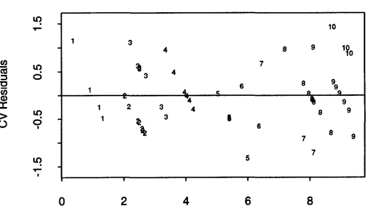
Figure 10. Cross-validated residual plots for non-linear models, (a) extremal spline

Figure 1. Examples of friction profiles

•

·

..

• ••

...

....

..

..

•

• # ••

..

•

..

.. ..

..

..

.

..

•

..

ex>

o

<0

o

• •

•

..

•

..

.. ..

..

•

..

•

...

•

•

..

...

.

•

•

•

..

•

•

..

.

•

•

•

• •

•

+ .+

•

•

grade=1

•

••• + + +++

...

_{#• • • •}

..

~ + .+

.+.

+ to. .~.+ .+ + +++ ~ +..+ ++ + +

+.... •...

." ..." . ,... •t.,\~

".to¥....~ ~

•

•

•

..

•

•

•

..

•

•

•

+ : + + + + + • • • ++ + ...

•

•

..

+

..

+

•

•

•

..

•

•

..

Q) ~

o

u..

•

C\I

o

o

o

Y~'t&\,

!

~rade=6

.

.

.,-:

....

~~

...

_/-/I

grade=10

~:.

. . . . ._

-D D D D

:

.I D

Figure 2. Extremal and quantile spline fits to a grade 1 friction profile

Extremal splines

ex>

o

o

o

o

100

200

Velocity

300

Q)

~

o

U-ex>

o

o

o

50;0

and

950;0

quantile splines

Figure 3. Linear classification model selection:

features from extremal splines

GCV

statistics

...

0 t: Q) c: 0 a>

*

'';:: 0 6 Co)

+

:a

~ +

=

a. r--. 36

Q) c::i + C) +

f

~ + + Q) _36A +

$

₊

*

:j:

!

+123456789AB

> 346A

ctI _{+ ~ + 123451S789A}

"0 L() 1356A 1 6At34567A 12345678A

Q) _c::i 1345678A

CiS E -.;::; _'=t (/J c::i

w

1

3

5

7 9 11

Number of variables

Cp

statistics

+ 0 ₆

t

L() ~

$

+

Co) _/+ +

'';::

36A

=

(/J

~ 0 346A

-

_(/J

...

a. () L()

...

+ :j: + + + +

; • + + :

~123456789AB

+ _± + + 123451S789A

1356A 134S6'i34567A 12345678A 1345678A

Figure 4. Linear classification model selection:

features from quantile splines

GCV

statistics

l -e l I -Q) c::: e +:: _en

t

(,) ci 8

:c

+

e

+ +

C. +12345678SAB

Q)

18 ~ 1345et8SAB

~

I""- + 1345;aSAB

ci +

38!B 38JAB

134~SAB

Q)

-

Ii

134!9AB

~ 38A 34 AB

"0 <0 Q) ci

c;

E '';:: IJ') CIJ ci w

1

3

5 7 9 11

Number of variables

Cp

statistics~ 0 c::i IJ') 8 _$ +

:I: + +

(,) _:ta

*

₊

*./

$

~123456789AB

+ ₊ .1345 89AB

+:: _{+ + 1345 SAB}

CIJ + +

.~ ₀ + 13488SAB

+

+ 134119AB

-

CIJ Lri ;

+

34~AB

C. ; :j:

c.:> 38A :j: 38SAB 38AB IJ') ci

Figure 5. Residual plots for linear models

Residuals from both models

Q)

"0

o

E

Q)

05 Q.

(/)

~

; ;

c

aj

:J C"

E

e

-...

10

o

10

o

I

Lq

...

I

-1.0

-0.5

0.0

0.5

1.0

1.5

-

C"

I

Q)

-

(/)

(ij

:J

"0

Ow

~

.5

Q)

o c

~

~

C

...

Residuals from extremal spline model

Figure 6. Comparison of extremal and quantile spline estimates of a grade 3 syringe

Envelope based on extremal splines

U!

..

"":

..

C\!

..

CD

e

If

..

C!

co

0

U!

0

0.0 0.02 0.04 0.06

Veloclly

0.08 0.10 0.12

Envelope based on 5% and 95% quantile splines

U!

..

"":

..

C\!

..

CD e

If C!

..

co

0

U) 0

0.0 0.02 0.04 0.06

Velocity

0.08 0.10 0.12

Estimated second derviative for the upper boundary

Figure 7. Non-linear classification model construction:

features from extremal splines

Residual plot for linear model

LO ₁₀

T"" ₁₀

9

3

4 9

LO 3 4 9 ₁₀

en _ci 2 9

cti

•

7

'aft

~ _1. 3 9

"'C

"(ij

.

..

Q)

LO

\

3 8

a:

_ci 3 ₄ 5

5 6 ₈ 9

I ₅

"

4

6 ₉

LO 5

T""

I

2 4

6

8 10

Predicted Grades

Spline estimate of transformation

o

T""

C\I

Figure 8. Non-linear classification model construction:

features from quantile splines

•

Residual plot for linear model

LO 10

~

3 9 1?0

2

,

4 8 9

en ~ 9

as

0 ₄ 8 9

:::J 11 ₂ 3

.,

_{\. 9}

"'C

88

0iij

~ 9

Q)

LO 2

a:

_ci 2 3 8 ₉

4

I _{3 5}

6

,

7

~ 6 7

~ 5

~

I

2 4 6 8

Predicted Grades

Spline estimate of transformation

o ~

Figure 9. Residual plots for non-linear models

•

Extremal spline model

LO

...

3 4

LO 3 4

C/) _{ci 2}

44

as

::3 3 5

" A

'0

"0 1 1 2 .. 4 5

CD _{LO 2'2:1} 3₄

a:

_ci 1 2 2 3

I 5 6 7 LO

...

I 9 10 10 7 9 10 9 88 9 "

..

8 9 8 8 8 99 78

2 4 6 8

Predicted values from non-linear model

Quantile spline model

LO

...

10

4 9

3 8 1'\9

LO _~ 4 ₇

C/) _ci

ca

3 8 ₉

::3 2 4 44 5 9

'0

..

"0 1 4

'"

5 6 81:1 "

CD 3 8 9₉

LO 1 2

a:

_ci 22 3 ₅ 8 9

I _{2 I} 6

7 8

7

LO

...

I

Figure 10: Cross-validated residual plots for non-linear models

•

Extremal spline model

T

LO

,...

_1Rl

9

3 3 ₇

f/) 4 10

as

It? 2 4 9

:::J 0

4l 9

"C

•

9

"Ci:i 3 ~ ~ A

Q) 1

"

5

u,

a:

\

₃ 4

LO 1 5

>

_{0 ~} 3 8 9

U I 4 8

3

6 77 8 9

LO 5

,...

I

2

4

6 8

Predicted values from non-linear model

Quantile spline model

It? ₁₀

,...

3 9 1?0 4 8 f/)

LO

,

7

as

4

:::J 0 3

"C ₆ 8 9

"Ci:i 4. _"

..

9"

Q) ₄

,

9

a:

1 2 3 _{4 9}

>

LO

3

•

8

0 1 _~

A

U I 6

\

8 9 7 7 It? 5

,...

I