Analysis and Modeling of Wave-current Interaction

(1)

ABSTRACT

LIU, HUIQING. Analysis and modeling of wave-current interaction. (Under the direction of Dr. Lian Xie).

(2)

(3)

Analysis and modeling of wave-current interaction

By

Huiqing Liu

A dissertation submitted to the Graduate Faculty of North Carolina State University

In partial fulfillment of the Requirements for the degree of

Doctor of Philosophy

Marine, Earth and Atmospheric Sciences

Raleigh, NC 2006 Approved by:

Dr. Leonard J. Pietrafesa Dr. John M. Morrison

Dr. Gerald S. Janowitz Dr. Lian Xie

(4)

DEDICATION

To my wife, Yao Liu. Without her love, encouragement and support, I couldn’t have

(5)

BIOGRAPHY

Huiqing Liu was born on the 11th of May, 1976, in AnQiu a city of Shandong province. In 1995, he was enrolled to Ocean University of Qingdao (now called Ocean University of

China), where he spent seven years in the Department of Oceanography and graduated with a

BS degree in 1999 and a MS degree in 2002. He joined the Department of Marine, Earth and

Atmospheric Sciences of North Carolina State University in fall 2002 as a graduate student

(6)

ACKNOWLEDGMENTS

I got much help from many great people during this work. Here, I wish to acknowledge

these great people, without their help, this dissertation would not have been possible. First, I

wish to express my extreme gratefulness to my advisor Dr. Lian Xie, whose knowledge,

guidance and kindness gave me much help throughout my time at NCSU. His encouragement

and patience led me step-by-step to complete this work. I also acknowledge the other

committee members: Dr. Pietrafesa, Dr. Morrison and Dr. Janowitz for their assistance and

comments to this study.

I also would like to thank my friends in the Coastal Fluid Dynamics Laboratory: Dr.

Machuan Peng, Dr. Shaowu Bao, Dr. Shiqiu Peng, Dr. Tingzhuang Yan, Dr. Xiaoming Liu,

Dr. Binyu Wang, Dr. Kristen Foley, Xuejin zhang, Meng, Xia and Yanyun Liu for their help

and suggestions in this study. Many thanks are also given to Bob Bright, Joshua Palmer,

Mike Lin and Sondra Artis for their help in my English pronunciation and writing skills.

I would also like to say thank you to my parents, Xinai Zhang and Junming Liu, and my

brothers, Huidong Liu and Huisheng Liu, for your tremendous love and financial support

throughout my life.

This study is supported by the Carolina Coastal Ocean Observation and Prediction

System (Caro-Coops) project under NOAA Grant No. NA16RP2543 via the National Ocean

Service, through Charleston Coastal Services Center. Caro-COOPS is a partnership between

(7)

LIST OF TABLES

Table 2.1 The water depth of buoy data stations get from different resolution topography.

Where Bias equal water depth get from topography minus actual water depth; ∈=

Bias/actual water depth..………..… … … …… ………..22

Table 3.1 List of experiments carried out in the study………...56

Table 4.1 List of experiments.………...……….89

Table 5.1 List of experiments.………...123

Table 5.2 Difference of flooding areas (total) among experiments.………124

(12)

LIST OF FIGURES

Figure 2.1 Computational domain, distribution of Buoy data stations and the best tracks of

hurricane Bonnie, Dennis and Floyd… … … …… …… … …… …… 23

Figure 2.2.1 a) The mean wave direction along the center line from deep water to coastal

line. The asterisk is the analytical solution and lines are results of SWAN.

Dashed line is swell wave with peak wave direction 450 and solid line is swell wave with peak wave direction 150. b) Water depth (m) along the center line..24 Figure 2.2.2 a) The mean wave direction and b) significant wave height along the center line

from deep water to coastal line. Solid line is the result of swell wave propagates

on the beach without any channels; dashed line is the result of swell wave

propagates on the beach with a channel without considering diffraction effect

and dotted line is considering diffraction effect. c) water depth (m) along the

center line…… … …… … … …… …… … …… … … … …... 25

Figure 2.2.3 Same as Figure 2.2.2 but for case 3. … … … …… …… … …… ……..26

Figure 2.3.1 Significant Wave height (SWH) at buoy data stations for hurricane Bonnie Solid

line is buoy data, dashed line is WAVEWATICH-III results and dot-dashed line

is SWAN results. X-axis is time (hour) and Y-axis is SWH (meter) …… ….. 27

Figure 2.3.2 SWH at buoy data stations for hurricane Bonnie. Solid line is buoy data, dashed

line is SWAN results and dot-dashed line is SWAN (depth-induced wave

breaking not be included) results…… … …… … … …… ……. 28

Figure 2.4.1 Same as Figure 2.3.1 but for hurricane Dennis. … … … …… …… … 29

(13)

Figure 2.5.2 Same as Figure 2.3.2 but for hurricane Floyd... … … … …… …… … 32

Figure 2.6 The original and shifted track of hurricane Floyd. Dashed line is original track

and solid line is the shifted track, which shifted to right 1o… … … ….. 33 Figure 2.7 SWH at buoy data station for modified hurricane Floyd by shifting track to right

1o. Dashed line is WWATCH-III results and solid line is buoy data… … ….. 34 Figure 2.8 The setup of nesting domain. The outermost domain covers from 200 to 400 N and 850 to 600 W with resolution 12 minute. The mid domain is 280-350 N, 820 -700W with 4 minute as the spatial grid size. The inner most domain is 310-340N, 81.50-76.50W with resolution 2 minute... … … … …… …… ………... 35 Figure 2.9 SWH at buoy data stations for hurricane Floyd. Blue solid line is buoy data, red

solid line is Swan coarse run result, black solid line is WaveWatch III coarse

run and blue dash line is Swan nested in WaveWatch III run… … … … ….. 36

Figure 2.10 SWH at buoy data stations for hurricane Floyd. Dashed line is the results of

outer domain, dotted line is med domain, dot-dashed line is inner domain and

solid line is the buoy data … …… … … …… ………. 37

Figure 3.1 a) Computational domain and Gulf Stream current field simulated by HYCOM.

One line traversing the Gulf Stream is from 80.60W to 79.40W longitude and latitude is 30.20N; b) The profile of current speed (y direction) along this line.57 Figure 3.2 a) Significant wave height (NE wind condition) variation between including the

effect of the Gulf Stream (Solid line) and without the Gulf Stream (dashed line)

along the line; b) Same as a) but for mean wave direction; c) two-dimensional

(14)

condition. The location of this spectra is 800 west longitude and 30.20 north latitude (location B in Figure 1b); d) same as c) but including current………58

Figure 3.3 a) Same as figure 3.2b but for swell wave case; b) and c) same as figure 3.2c and

3.2d but for swell case………59

Figure 3.4 a) Same as figure 3.2a but under SE wind condition; b) two-dimensional spectra

of wind waves with and without current under SE wind condition at location A

(shown in Figure 3.1b); c) same as b but for location B; d) same as b but for

location C; e) same as figure 3.2b but under SE wind condition………60

Figure 3.5 a) Same as figure 3.3a but main swell direction is SE; b) and c) same as figure

3.2b and figure 3.2d but for swell case………..62

Figure 3.6 a) Same as figure 3.2a but for east wind condition; b) same as figure 3.2b but for

east wind condition……….…………63

Figure 3.7 a) Same as figure 3.5a but main swell direction is east; b) same as figure 3.5b

but for location B and main swell direction is east………65

Figure 3.8 The distributions of the best track of hurricane Bonnie (1998), the buoy data

station and the observation points of SRA………..66

Figure 3.9 a) Significant Wave Height induced by hurricane Bonnie at buoy data station 4-

1002, 41004 and Fpsn7. Solid line is the result of SWAN model including the

Gulf Stream effect, dashed line is the result of SWAN model without

considering the Gulf Stream effect and star point is buoy data………..67

Figure 3.10 The peak wave direction along the sample SRA points under hurricane Bonnie

(15)

results without considering the effect of the Gulf Stream and black square

represents model results considering the effect of the Gulf Stream…………...68

Figure 4.1 The distribution of significant wave height (SWH) driven by static symmetric

hurricanes (a) and symmetric hurricanes with different translation speeds b) 2

m/s; d) 4 m/s; f) 6 m/s; h) 8 m/s; j) 10 m/s; i) 12 m/s and different SWH

differences between them and these generated by the static hurricane c) 2 m/s;

e) 4 m/s; g) 6 m/s; i) 8 m/s; l) 10 m/s; m) 12 m/s………...90

Figure 4.2 The locations of two points. Point ‘A’ locates in the first quadrant one RMW

from the storm center, while point ‘B’ locates in the third quadrant, also one

RMW away from the storm center………..91

Figure 4.3 SWH values of waves generated by symmetric hurricanes moving with different

translation speeds of location ‘A’ a) and location ‘B’ b) (shown in Figure 4.2) at

MWRs……….92

Figure 4.4 One dimensional directional wave spectrum at Point A, which were generated b-

y symmetric hurricanes moving with different translation speeds: a) 0 m/s; b) 2

m/s; c) 4 m/s; d) 6 m/s; e) 8 m/s; f) 10 m/s; g) 12 m/s and h) 14 m/s………….93

Figure 4.5 Same as Figure 4.4 except for Point B……...……….94

Figure 4.6 Schematic picture of swell (of Point A and Point B) propagating in the direction

tangential to the circle defined by the RMW at an earlier position of storm…..95

Figure 4.7 SWH values of waves generated by static and symmetric hurricanes with differ-

ent intensity of location ‘A’ a) and location ‘B’ b) (shown in Figure 4.2) at

(16)

Figure 4.8 Normalized SWH difference (NSD) at location ‘A’ a) and location ‘B’ b)

(show-n i(show-n Figure 4.2)...97

Figure 4.9 The model topography and domain used in experiment D, extends latitudinally

from 25o to 35o north and longitudinally from 85o to 70o west. Dashed-X line and solid-point line are the best tracks of Bonnie and Floyd respectively. The

X-mark is the distribution of the buoy data stations………...98

Figure 4.10 a) The distribution of symmetric hurricane wind fields (Bonnie) at 18:00 of Aug.

25, 1998; b) Same as a) but for asymmetric hurricane wind and c) The

difference between these two wind fields………...99

Figure 4.11 a) The distribution of SWH generated by symmetric hurricane wind (Bonnie) at

18:00 of Aug 25, 1998; b) Same as a) but driven by asymmetric hurricane wind

and c) The difference between these two SWH fields………..100

Figure 4.12 SWH values during hurricane Bonnie at buoy data station a) 41002; b) 41004

and c) Fpsn7. Solid line is buoy data, dashed line is model results driven by

symmetric hurricane and dotted line is model results driven by asymmetric

hurricane wind………..101

Figure 4.13 Wind speed during hurricane Floyd at buoy station a) 41004; b) 41008 and c)

Fpsn7. Solid line is buoy data, dashed line is the result of asymmetric hurricane

model and dot-dashed line is the result of symmetric hurricane model……...102

Figure 4.14 Same as Figure 4.13 but for SWH field…...……….103

Figure 5.1 Flow diagram illustrating the coupling process between the wave and current

model……….125

(17)

Figure 5.3 a) Locations in the study area where data are used to plot the peak surges in

panel b). b) Peak storm surges at the locations shown in a) for Case NN (green)

and YYR (red)………127

Figure 5.4 Simulated maximum flooding areas induced by Hugo of case NN. The green color represents the maximum flooding areas………...128

Figure 5.5 (a) Simulated maximum flooding areas induced by Hugo of case YN……….129

Figure 5.5 (b) the different maximum flooding areas between case YN and NN (case YN – case NN). The dark red color represents the shoreward increase flooding areas and the light green color represents the reduced flooding areas………...130

Figure 5.6 The definition of North, East and Southwest regions………131

Figure 5.7 (a) Same as Figure 5.5(a) but for case NY………132

Figure 5.7 (b) Same as Figure 5.5(b) but for case NY………133

Figure 5.8 (a) Same as Figure 5.5(a) but for case NNR……….134

Figure 5.8 (b) Same as Figure 5.5(b) but for case NNR……….135

Figure 5.9 (a) Same as Figure 5.5(a) but for case YYR……….136

(18)

CHAPTER 1. INTRODUCTION

1.1Scientific Background

Wind-generated waves are the prime energy supplier to the nearshore area, generating

currents and transporting sediments, so shaping our coasts. It is logical therefore that they are

a prime subject of research in physical oceanography and coastal engineering, which has led

to significant advances in understanding as well as modeling capability. Prediction of wind

waves in extensive areas such as oceans and shelf seas is only practically feasible in a

phase-averaged sense. This has led to numerical models based on the spectral wave energy balance,

with linear propagation and a set of source terms accounting for wind input, cross-spectral

transfer and dissipation. The archetype model in this category is WAM [WAMDI Group,

1988; see also Komen et al., 1994], primarily developed for deep water, with some

allowances for restricted depth. WAVEWATCH (WW) [Tolman, 1991] is a similar model,

while the model SWAN, based on the same principles, is designed especially for shallow

coastal regions [Booij et al., 1999]. The prediction skill of these models has been

demonstrated in many experimental exercises. Generally the skill of wave prediction is

mainly determined by wind field input as well as boundary condition, current condition and

topography (depth-induced breaking). For example, when waves encounter a strong current

(e.g. Gulf Stream), the changes of wave height and direction induced by current will be

significant, and wind is the principal source of energy creating and driving waves. Therefore

(19)

Wind waves, storm surges and ocean circulation are important, mutually interacting

physical processes in coastal waters. Over the past two decades, there have been a number of

studies focusing on wave-current interactions [Tolman, 1990, Zhang and Li 1996, Xie et al.

2001, 2003]. It is believed that wind waves can indirectly affect the coastal ocean circulation

by enhancing the wind stress [Mastenbroek et al., 1993] and by influencing the bed friction

coefficients [Signell et al., 1990, Davies and Lawrence, 1995]. Xie et al. [2001, 2003] studied

wave-current interactions through surface and bottom stresses and found that wind waves can

play a significant role in the overall circulation in coastal regions.

The key questions here must address how these processes affect one another and how

these processes can be properly coupled in numerical models. In general, these processes

influence one another in several ways: (1) wind stress, which is changed by incorporating the

wave effect [Donelan et al., 1993]; (2) radiation stress, which is considered to be an

additional mechanical force in storm surge models [Xie et al., 2001, Mellor, 2003, Xia et al.,

2004] and can be incorporated into wave models by invoking wave-action conservation

[Komen et al., 1994, Lin and Huang, 1996]; (3) bottom stress, which is a function of

wave-current interaction in the near bottom layer when the water depth is sufficiently shallow for

wave effects to penetrate to the bottom [Signell et al., 1990]; (4) the depth variation and

current conditions, which are inputted into wave models [Tolman, 1991]; (5) the Stokes’ drift

current induced by the non-linearity of surface waves [Huang, 1979]; and (6) wave run-up,

which has an impact on storm surge and inundation prediction [Holman et al., 1985 and

(20)

Because of the importance of these interactions, there have been several studies which

have attempted to incorporate these separate but important and linked effects into coupled

models. Tolman [1991] described the effects of astronomical tides and storm surges on wave

modeling via the consideration of unsteady currents and varying topography. Tolman’s

results suggest that the effects of tides and storm surges should be considered in modeling

physical waves in shelf seas. Tolman’s insightful study assumed one-way coupling and did

not consider the effect of wind waves on storm surge. Signell et al. [1990] studied the effect

of waves on bottom shear stress and Davies and Lawrence [1995] showed that wind waves

could play an important role in determining surface and near bottom currents as well as on

water level variations over and along a coastal region. In the Signell et al and Davies and

Lawrence studies, surface waves were considered to be a constant external input into the

current model, a one-way coupling.

Xie et al. [2001, 2003] investigated the dynamic coupling between waves and currents

and found that it was important to incorporate the surface wave effects into coastal

circulation and storm surge modeling. The results of their study showed an improved storm

surge prediction capability. However, they did not consider depth variations in their wave

model, which limited the more complete application of their results. Moon [2005] also

developed a wave-tide-circulation coupled system, in which the effects of wave-current

interactions on surface stress, a wave breaking parameterization, and depth variations in their

wave model were included. However, the effects of wave-current interaction on the bottom

shear stress were not included. Moreover, all of the above mentioned storm surge models did

(21)

et al., 2004] and did not include inundation as part of their storm surge model architecture.

Flooding caused by coastal storms is an occasional threat to people living in coastal regions.

So it is important to investigate the effect of wave-current interaction on coastal atmospheric

storm induced storm surge and inundation.

1.2Purposes of the Study

Ocean waves play an important role in the transfer of momentum and energy across the

air-sea interface and strongly impact current, storm surge and coastal inundation flooding.

Specifically, waves generated by hurricanes are relatively large and can easily reach 10-20

meters or even larger in sufficiently deep open ocean waters. Although the waves reduce

their SWH when they reach the shallow water areas, they can still significantly impact the

coastal zone. High waves can create hazardous conditions including debris overwash,

flooding, erosion, high wave energy and turbulence in the nearshore zone, and strong

currents. It is well known that hurricane waves are one of the most damaging phenomena

during the passages of hurricanes. Severe wave conditions are dangerous to vessels in ocean

and coastal waters, and waves can also run up over the storm surge in the coastal zone to

cause more severe damage along and on the coast, for example it can overwash coastal roads

and properties. So the ability to predict hurricane waves precisely is a very important

challenge and is of great value to many user communities.

To predict hurricane waves, you have to quantify the sensitivity of waves to several

(22)

hurricane wind fields. In order to address this issue, a suite of study topics are designed to

quantify the influence of: 1) depth-induced refraction-diffraction, wave breaking and spatial

resolution; 2) major western currents (e.g. Gulf Stream); 3) wind distribution, storm

translation speed and intensity on ocean surface wind waves using SWAN.

As shown in the first section of this chapter and previous studies, wind waves have an

important role in storm surges, inundation and ocean circulation in coastal waters. Generally,

surface waves and currents influence one another in several ways: 1) wind stress, which is a

function of the drag coefficient which is strongly tied to wave parameters [Donelan et al.,

1993]; 2) the radiation stress, which is considered to be an additional mechanical force in

storm surge models [Xie et al., 2001, Mellor, 2003, Xia et al., 2004] can be incorporated into

wave models by invoking wave-action conservation [Komen et al., 1994]; 3) the bottom

stress, which is a function of wave-current interaction in the near bottom layer when the

water depth is sufficiently shallow for wave effects to penetrate to the bottom [Signell et al.,

1990]; 4) water depth variation and current conditions, which are input parameters for the

wave models [Tolman, 1991]; 5) the Stokes’ drift current induced by the non-linearity of

surface waves [Huang, 1979]; and 6) wave run-up, which impacts storm surge and

inundation prediction [Holman et al., 1985 and 1986].

Therefore, we will develop a three-dimensional (3-D) wave-current dynamic coupled

modeling system, including the effect of wave-current interaction on storm surge and

(23)

surface wind stress, wave-current-dependent bottom shear stress, and time-dependent sea

surface elevation in the wave model, and three-dimensional radiation stress.

1.3Organization of dissertation

Investigation of depth-induced refraction-diffraction, wave breaking and nesting impacts

on waves using SWAN are given in chapter 2. Chapter 3 introduces a numerical study on the

effect of the GULF STREAM on waves. Sensitivity of near-shore wind waves to hurricane

wind asymmetry and translation speed are investigated in chapter 4. The effect of

wave-current interactions on the storm surge and inundation in CHARLESTON harbor during

(24)

CHAPTER 2. INVESTIGATION OF DEPTH-INDUCED

REFRACTION-DIFFRACTION, WAVE BREAKING AND

NESTING IMPACTS ON WAVES USING SWAN

2.1.Introduction

Simulation WAves Nearshore (SWAN) [Booij et al. 1999] and WAVEWATCH-III

[Tolman, 2002] are the third-generation wave models, which solve the spectral action

balance equation without prior assumption of spectral shape. The prediction skill of these

models has been demonstrated in many experimental cases [Ris et al., 1999, Rogers et al.,

2003, Hsu et al., 2005, Zijlema and Westhuysen, 2005, Tolman, 1991]. There are many

factors that affect their performance in prediction, e.g. spatial resolution, dissipation and

wind fields. Especially in coastal areas, depth-induced refraction-diffraction and wave

breaking is important for wave prediction due to shoaling effect. In simulating hurricane

induced waves, wave models frequently yield inordinately high values of wave heights in

shoal areas if wave breaking effect is not taken into account in models. This is also one of

driving forces to develop SWAN wave model. The main purpose of developing SWAN

model is to obtain realistic estimates of wave parameters in coastal areas, lakes and estuaries

from given wind, bottom and current conditions [SWAN Group, 2003]. Hence, the

depth-induced refraction-diffraction [Holthuijsen et al., 2003], wave breaking [Booij et al. 1999]

(25)

determine in which domain depth-induced refraction-diffraction should be considered, in

which domain depth-induced wave breaking should be activated and in which domain fine

grids should be selected; whereas some domain coarse grids could be ok.

Many studies have been focused on the wave breaking effect, e.g. Battjes and Janssen

[1978] presented a wave breaking dissipation approach, in which the local mean rate of

energy dissipation is modeled. The results of their models indicated a good agreement with

field experiments. The calibration and verification of their model was conducted by Battjes

and Stive [1985] using both laboratory and field data. Massel and Gourlay [2000] developed

a model which predicted wave transformation and wave-induced set up on coral reefs. Two

energy dissipation mechanisms had been incorporated into that model, i.e., wave breaking

and bottom friction. Considering waves on shallow foreshores are subject to depth-induced

breaking, Battjes and Groenendijk [2000] proposed a Composite Weibull distribution to

describe the wave height distributions on shallow foreshores. Zhao, et al. [2000] developed a

two-dimensional wave model which included wave breaking effects to simulate three cases.

The results showed that wave height in the nearshore areas was higher obtained from

Non-wave breaking than Non-wave breaking results. As the Non-wave breaking is one of important

dissipation aspects in shallow water areas, it suggests that switching off the depth-induced

breaking term is usually unwise, since that leads to unacceptably high wave heights (the

computed wave heights ‘explode’ due to shoaling effects) [SWAN user manual]. At the same

time, waves may be refracted and diffracted due to the presence of shoals and channels or

obstacles such as islands, headlands, or break waters when they approaching a coastline

(26)

numerical model in order to obtain realistic simulating results around coastal areas. The

widely used methods accounting for diffraction effect in models are mild-slope model

[Berkhoff, 1972, Ito and Tanimoto, 1972, Gao and Radder, 1998] and Bossinesq model

[Madsen and Sørensen, 1992, Li and Zhan, 2001]. In SWAN model, the effects of refraction

and diffraction are readily accounted by adding the diffraction-induced turning rate of the

waves (obtained from mild-slope equation) to model.

So far, there are few studies which focus on investigating the effect of wave breaking

dissipation on waves induced by a Hurricane, and few studies focus on examining the

conditions controlling this effect on waves, i.e., did wave breaking effect play the same role

on waves throughout the domain? In this chapter, we will discuss the wave breaking how to

affect the wave height during hurricane passing the domain, test the effect of depth-induced

refraction-diffraction incorporated into SWAN and examine the spatial resolution effect on

wave field using nesting method. SWAN and WAVEWATCH-III wave models were used to

simulate several real hurricane cases in our experiment in order to investigate the

depth-induced wave breaking and spatial resolution impacts on waves, in which the hurricane fields

were simulated by Holland hurricane model [Holland, 1980]. At the same time, several ideal

experiments were conducted to examine the impacts of depth-induced refraction-diffraction

presented in SWAN on waves. Wave models and hurricane model employed in this chapter

are described in section 2.2. Section 2.3 introduces ideal and real hurricane experiments,

model domains and buoy data stations used in this chapter. Section 2.4 provides experiment

(27)

cases (wave breaking and nesting effect). Discussions and summary are presented in section

2.5.

2.2.Models description

2.2.1 SWAN

The model is based on the wave action balance equation (or energy balance in the

absence of currents) with sources and sinks. In SWAN the evolution of the wave spectrum is

described by the spectral action balance equation which for Cartesian coordinates is (e.g.,

Hasselmann et al., 1973):

σ θ σ σ θ S N C N C N C y N C x N

t x y ∂ =

∂ + ∂ ∂ + ∂ ∂ + ∂ ∂ + ∂ ∂ (2.1)

Where N is the action density (N(σ, θ) = E(σ, θ) / σ), E is the energy density spectrum and σ

is the relative frequency. Cx, Cy and Cσ are propagation velocity in x-, y-, σ- and θ-space

respectively. S is the source term that represents the effects of generation, dissipation and

nonlinear wave-wave interactions. The governing equation is expressed in spherical

coordinates is: σ θ σ ϕ ϕ ϕ λ λ ϕ σ θ S N C N C N C N C N

t ∂ =

∂ + ∂ ∂ + ∂ ∂ + ∂ ∂ + ∂

∂ _(cos ₎−1 _cos

(2.2)

Where λ and ϕ represent longitude latitude respectively.

Depth-induced wave breaking has been considered in SWAN, which is expressed by the

(28)

2 ) 2 ( 4 1 m b BJ

tot Q H

D π σ α − =

in wich αBJ = 1 and Dtot is the mean rate of energy dissipation per unit horizontal area due to

wave breaking. It is based on the bore-based model of Battjes and Janssen [1978]. Qb is the

fraction of breaking waves determined by: 8 ₂

ln 1 m tot b b H E Q

Q ₌₋

−

in wich H m is the maximum

wave height that can exit at the given depth.

2.2.2 WAVEWATCH-III

WAVEWATCH-III was developed at the Marine Modeling and Analysis Branch

(MMAB) of the Environmental Modeling Center (EMC) of the National Centers for

Environmental Prediction (NCEP) [Tolman, 2002] in the spirit of the WAM [WAMDI group,

1998]. It is the operational ocean wave predictions model of NOAA/NCEP, in which the data

assimilation is included. WAVEWATCH-III solves the spectral action density balance

equation for wave number-direction spectra. The implicit assumption of this equation is that

properties of medium (water depth and current) as well as the wave field itself vary on time

and space scales that are much larger than the variation scales of a single wave.

(http://polar.ncep.noaa.gov/waves/wavewatch/wavewatch.html) The governing equation is:

σ θ θ S N N k k N x t N

x _∂ =

∂ + ∂ ∂ + • ∇ + ∂

∂ _& _&

& (2.3)

U C

x& = _g + (2.4)

s U k s d d k ∂ ∂ • − ∂ ∂ ∂ ∂ − = σ

(29)

    ∂ ∂ • − ∂ ∂ ∂ ∂ − = m U k m d d k σ

θ& 1 (2.6)

K and θ are wave number and propagation direction, respectively. s is a coordinate in the

direction θ and m is a coordinate perpendicular to s. The main difference between the two

wave models is that parameterizations of physical processes included in WAVEWATCH-III

model do not address conditions where the waves are strongly depth-limited.

2.2.3 Holland hurricane model

The wind speed is the function of radial distance from the center of the storm described

as:

[ ( )exp( / )/ a B]1/2 B

c

n P A r r

P AB

V = − − ρ _(2.7)

where V is wind speed at radius r, Pc is the central pressure of hurricane, Pn is the ambient

pressure, ρa is the air density, A and B are constants. In which Pn = 105 Pa, ρa = 1.2 kg/m3, B

= 1.9 and A = (Rmax)B. The value of Rmax depends on the value of Pc.

2.3.Experiments and model setup

In order to examine the influence of depth-induced refraction-diffraction on waves, three

ideal experiments (named case 1, 2 and 3) are conducted in this chapter. Only swell waves

(avoid other effects except refraction-diffraction effect) propagate from deep water to coastal

(30)

width of the Gaussian frequency spectrum is 0.007 Hz; the significant wave height is 1.2 m;

peak frequency is 0.071 Hz; peak wave direction is 150 or 450 in case 1 and 00 in case 2 and

3; the directional width is 12.40. All the angles used in this chapter are under Cartesian

convention. The domain of these ideal experiments is 45 km in x direction and 15 km in y

direction with 1 km grid size resolution of both directions. The water depth decreases from

50 m to 5 m in x direction and the water depth in y direction is uniform for case 1. There is a

sub-water channel and ridge at the distance 21~26 km from coastline in case 2 and case 3

respectively. For case 2, the depth of channel is 50 meter. On the other hand, the water depth

of ridge in case 3 is 8 meters.

Three real hurricane cases (Bonnie 1998, Dennis 1999 and Floyd 1999) are selected in this

chapter to examine the effect of depth-induced wave breaking and the influence of spatial

resolution on waves. The best tracks of these hurricanes are shown in Fig. 2.1. These tracks

data is provided by Unisys Weather Hurricane/Tropical data center. Figure 2.1 alsodescribes

the computational domain of these hurricane cases, which covers latitude from 25o to 35o

north and longitude from 85o_{to 70}o_{west. The bottom topography is derived from the ETOP5}

bathymetry database. The resolution of both wave models is 1/5o in both directions. The last

information presented in Fig. 2.1 is the distribution of buoy stations, in which data was used

to compare with model results.

2.4.Results

2.4.1 The effect of depth-induced refraction-diffraction on waves

The effect of depth-induced refraction-diffraction plays an import role on waves

(31)

encounter sub-water channels or ridges. That is why these effects are incorporated into most

wave models. In this section, several ideal experiments were conducted to investigate these

processes represented in SWAN.

The results of the first ideal experiment (case 1) are illustrated in Fig. 2.2.1. In this case,

swell waves propagate through a plane beach with a slope 10-3 in the depth range from 5 to

50 m. Two swell waves are considered in this case, one propagates with peak wave direction

450 and the other is 150. Figure 2.2.1a shows the variation of mean wave direction due to

depth-induced refraction on the plane beach including model and analytical results. It

indicates that depth refraction makes waves bend toward to the normal direction of beach (00)

and shows a good agreement with the analytical results (symbols in Fig. 2.2.1a). The

analytical results are calculated by using Snel’s law:

, sin

const

c =

θ

c k

σ =

(2.8)

Where θis the wave direction, c is the wave phase speed, σis the wave frequency and k is

the wave number. The constant is determined from the (deep water) boundary conditions.

To illustrate the influences of depth-induced diffraction on waves, two cases (case 2 and

case 3) have been considered. In case 2 (second ideal experiment), swell waves with peak

wave direction 0 propagate from deep water to a plane beach (same as the first case) but with

a sub-water channel. The setups of case 3 are the same as the second case except that there is

a sub-water ridge not a channel in the beach. Figure 2.2.2 presents the results of the second

(32)

suggests that diffraction makes waves propagate closer to their original direction (reduced the

effect of channel) during through and after passing the channel. Furthermore it increases the

wave height of the back areas of channel (Fig. 2.2.2b). In Fig. 2.2.3 the results of case 3 are

presented. As the same anticipated, the modulation of wave propagation (Fig. 2.2.3a) and

wave height (Fig. 2.2.3b) due to the diffraction is obvious. Whereas Figure 2.2.2 and Figure

2.2.3 indicate that the effects of diffraction are to enhance the energy penetrates into the areas

behind the sub-water channel or ridge. In other words, the impacts of diffraction help reduce

the influence induced by sub-water channel or ridge on waves.

2.4.2 The effect of depth-induced wave breaking on waves

To explore the depth-induced wave breaking and spatial effects on wave field, three real

hurricane cases were selected as the forcing fields of SWAN and WAVEWATCH-III wave

models. The best tracks of these hurricanes are shown in Fig. 2.1 which includes Bonnie

(1998), Dennis (1999) and Floyd (1999). Hurricane wind fields of each case was simulated

by Holland hurricane model [Holland, 1980] and inputted into wave models. Wave fields

induced by the same hurricane were simulated three times by the two wave models. The first

two simulations were conducted by SWAN and the difference between them is that one

switched on wave breaking term and the other switched off wave breaking term. And the last

one was simulated by WAVEWATCH-III.

Figure 2.3-Figure 2.5 show the significant wave height (SWH) induced by hurricanes at

(33)

Bonnie are shown in Fig. 2.3 including outputs of SWAN (switch on and off wave breaking

term) and WAVEWATCH-III and observed buoy data. Figure 2.4 and Figure 2.5 display

results of Dennis and Floyd hurricane case respectively. In view of these comparison, two

wave model results display a good coincidence with buoy data no matter whether the wave

breaking term on or off in SWAN at most of buoy stations for these three hurricane cases.

However, it can be noted that the results of WAVEWATCH-III and SWAN (wave breaking

term is off) are extremely higher than those of SWAN (including breaking term) and

observed data in station Fran Pan Shoals, NC (FPSN7) for hurricane Bonnie and Floyd

cases (Fig. 2.3c and Fig. 2.5d). The character of station FPSN7 is that its position is 33.49N

and 77.59W, which is very close to shore line, and its water depth is 20~21m. Therefore, the

reason of why SWH simulated by SWAN (wave breaking term is off) and

WAVEWATCH-III is poor may be that water depth of buoy station FPSN7 is shallow enough to consider

wave breaking dissipation. In other words, depth-induced wave breaking is an important

dissipation mechanism in shallow water regions, which should be incorporated into wave

models. Otherwise, numerical models would produce unrealistic results in these regions.

Whereas, the more interesting phenomenon is that the performances of

WAVEWATCH-III and SWAN (no wave breaking term) at buoy station FPSN7 are good for hurricane

Dennis case compared to buoy data. The apparent difference among these three hurricane

cases is the relative location of buoy station FPSN7 to the best track of hurricane. It can be

obviously noticed that the best track of hurricane Dennis passed through right of buoy station

FPSN7 (Fig. 2.1), however, buoy station FPSN7 lies in the right area of the best tracks of

(34)

(depth-induced wave breaking no considered) at buoy station FPSN7 will be extremely high

when it lies in the right of the best track of hurricane, however, this phenomenon will be

disappeared when buoy station FPSN7 lies in the left of the best track of hurricane. Why? It

is known that hurricane is a tropical cyclone system and its wind direction is shoreward at

upper-right quadrant (along east coast of North Hemisphere). Therefore waves induced by

the hurricane at this quadrant would propagate from deep water to coastal water. To the

contrary, the hurricane wind direction is seaward and waves induced by the hurricane will

propagate from coastal water to deep water at lower-left quadrant. It means that larger waves

(SWH is high) will propagate from deep water to shallow water at the right areas of the best

track of hurricane, whereas, small waves will propagate from shallow water to deep water at

the left areas of the best track of hurricane. Therefore, it is obvious that the effect of

depth-induced wave breaking would play a significant role in simulating waves at the right areas of

the best track of hurricane and not have the same impact on waves at the left areas. To verify

this explanation, an experiment had been conducted, in which the best track of Floyd was

shifted to right by adding 1o in west longitude named hurricane Floyd-fix for every point in

order to make it pass on the right of FPSN7. Figure 2.6 shows the positions of original and

modified best track of Floyd (hereafter named fix). All parameters of hurricane

Floyd-fix are the same as the hurricane Floyd except the passage of the best track. The SWH

induced by hurricane Floyd-fix at station FPSN7 is presented in Fig. 2.7. The result indicates

that there is no significantly difference between SWH simulated by SWAN (no wave

breaking and including its effect) and WAVEWATCH-III. Hence, the above explanation is

(35)

On the other hand, WAVEWATCH-III shows a better performance in station 41002

(water depth is about 3785 m) than SWAN does compared with buoy data, i.e.

WAVEWATCH-III has a better performance in deep water areas than SWAN (Fig. 2.3a,

Fig. 2.4a and Fig. 2.5a).

2.4.3 The effect of spatial resolution on waves

In order to investigate the impact of spatial resolution on wave fields, two nesting runs

were conducted for the hurricane Floyd case. The first one was SWAN nested in SWAN

itself run and the other one was SWAN nested in WAVEWATCH-III run. Figure 2.8 shows

the computational domain and the nesting windows: The outermost domain covers from 200

to 400 North and 850 to 600 West with resolution 12 minute. The mid domain is 280-350N,

820-700W with 4 minute as the spatial grid size. The inner most domain is 310-340N, 81.50

-76.50W with resolution 2 minute. Time step for integration is 6 minutes. Number of

frequencies of waves is 31 (0.04177~1.0 Hz) and directional resolution is 100 (00~3600).

As was indicated in the previous section of this chapter, WAVEWATCH-III doesn’t

perform as well as SWAN wave model does in shallow water areas but does better in deep

water (more efficient than SWAN). Hence, SWAN nested in WAVEWATCH-III run (first

experiment) could be used to study the effect of boundary condition on waves, in which the

mid domain and outermost domain were used. Except this experiment, SWAN nested in

SWAN run was conducted in these three nesting domains to study the effect of spatial

(36)

Same as the previous experiments, Hurricane Floyd was also simulated by Holland

hurricane model [Holland, 1980] and Buoy data was employed to compare with model

results. The results of the first nesting run are presented in Fig. 2.9. It shows that the

significant wave height simulated in nesting run (SWAN nested in WAVEWATCH-III) is

closer to WAVEWATCH-III (independent run) result during hurricane not approaching

computational domain; however, it bends to SWAN (independent run) result during

hurricane dominating the domain. The reason is that the wind speed is very small before the

front edge of a hurricane reaches the model domain (due to no background wind field

incorporated in Holland hurricane model) and wave energy is mainly transported from

boundary condition (supplied by the coarse run of WAVEWATCH-III). On the other hand,

wind will play much more important role in wave generation when hurricane effect reaches

the domain due to the large wind speed. Thus, the significant wave height simulated in the

first nesting run is mainly impacted by boundary condition when hurricane effect does not

enter the domain, whereas it will be controlled by wind forces during hurricane approaching

the domain. In other words, boundary conditions have little impact on waves (could be

disregarded) when wind forces are strong in computational domain.

In the second nesting run experiment (SWAN nesting itself), the results are displayed in

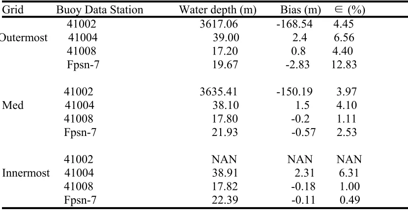
Fig. 10. Before describing the results, it is worthwhile to show the difference of the water

depth at buoy stations among gaining from different resolution bathymetry (Table 2.1). It

can be seen that the water depth at buoy data stations is various from grid to grid. Water

(37)

m, for innermost it is 17.82 m and actual water depth is 18.0 m. The water depth bias

indicated by table 2.1 is significant among different grids and the bias of outermost is

largest. Hence, the SWH values (Fig. 2.10) computed by the models show that the results of

outermost grid are the worst compared to buoy data, mid grid and innermost grid are better.

Furthermore, the results are improved more obviously from outermost to mid grid than from

mid grid to innermost. It suggests that the effect of bathymetry resolution should be

considered in wave prediction but not necessary to consider too fine grid resolution.

2.5.Discussions and summary

The depth-induced refraction-diffraction process presented in SWAN was tested using

several ideal experiments in this chapter. The results of the beach refraction experiment

indicate that depth-induced refraction has a significant impact on wave propagation; it also

shows a good agreement with analytical result. At the mean time, the influence of

depth-induced diffraction plays an important role in wave propagation and wave height when

waves cross a sub-water channel or ridge in a beach. The results of experiments show that

there is a significant impact on waves if we activating the diffraction option in the SWAN. It

suggests that it is important to consider depth-induced diffraction effect to compute the wave

field in some specific case.

The effect of depth-induced wave breaking is often neglected or not given regard enough

by researchers in their wave simulation. Especially in hurricane cases, there are fewer studies

(38)

including breaking term) and WAVEWATCH-III forced by hurricane was conducted in this

chapter. Three hurricane cases and one modified hurricane case were selected as examples to

examine the effect of wave breaking in shallow water area. In most cases, the results in

station FPSN7 are poorer compared with observation data if the effect of wave breaking is

not considered in wave models than the results that include this effect. However, the wave

models exhibit no much different prediction skill at station FPSN7 when the track of

hurricanes passed through its right area. Therefore, depth-induced wave breaking is not

always important in shallow water areas in hurricane-induced wave simulation case. It has

more significant impact on wave field in areas which lies on the right of hurricane than those

lies on the left of hurricane.

The effect of topography resolution on waves is important when bathymetry feature is

complex, which need fine grid to represent it. Otherwise, it is not necessary to pick too fine

grid resolution to compute wave field using nesting run. The effect of boundary condition on

waves depends on the wind conditions, it is significant during weak wind conditions but it

can be disregarded during peak wind conditions. That is to say, waves are mainly determined

by boundary conditions during hurricanes increase phase and hurricanes play the main role in

(39)

Table 2.1 The water depth of buoy data stations get from different resolution topography. Where Bias equal water depth get from topography minus actual water depth; ∈=

Bias/actual water depth.

Grid Buoy Data Station Water depth (m) Bias (m) ∈ (%) 41002 3617.06 -168.54 4.45 Outermost 41004 39.00 2.4 6.56 41008 17.20 0.8 4.40 Fpsn-7 19.67 -2.83 12.83

41002 3635.41 -150.19 3.97 Med 41004 38.10 1.5 4.10 41008 17.80 -0.2 1.11 Fpsn-7 21.93 -0.57 2.53

(40)

Figure 2.1.Computational domain, distribution of Buoy data stations and the best tracks of hurricane Bonnie, Dennis and Floyd.

-85 -80 -75 -70

25 26 27 28 29 30 31 32 33 34 35

(41)

4 k0 3 k 2 k 1 k k 5 10 15 20 25 30 35 40 45 M ea n W a ve D ir e ct io n ( 0) 450 150

45km 35km 25km 15km 5km

60 40 20 0 Wa te r D e p th ( m )

Distance from coast (m)

Figure 2.2.1. a) The mean wave direction along the center line from deep water to coastal line. The asterisk is the analytical solution and lines are results of SWAN. Dashed line is swell wave with peak wave direction 450 and solid line is swell wave with peak wave direction 150_{. b) Water depth (m) along the center line.}

a

(42)

45km 35km 25km 15km 5km -0.5 0 0.5 1 M ea n W a ve D ir e ct io n ( 0)

45km 35km 25km 15km 5km

0.9 1 1.1 1.2 S ign W a v e H eig ht ( m )

45km 35km 25km 15km 5km

60 40 20 0 Wa te r D e p th ( m )

Distance from coast (m)

channel-no Beach channel-Dif a b c

(43)

45km 35km 25km 15km 5km -4 -2 0 2 M ea n W a ve D ir e ct io n ( 0 )

45km 35km 25km 15km 5km

0.8 1 1.2 1.4 S ign W a v e H eig ht ( m )

45km 35km 25km 15km 5km

60 40 20 0 Wa te r D e p th ( m )

Distance from coastline channel-no Beach channel-Dif a b c

(44)

(45)

(46)

(47)

(48)

(49)

(50)

Figure 2.6. The original and shifted track of hurricane Floyd. Dashed line is original track and solid line is the shifted track, which shifted to right 1o.

-85 -80 -75 -70

26 28 30 32 34 36 38

(51)

Figure 2.7. SWH at buoy data stations for modified hurricane Floyd by shifting track to right 1o. Dashed line is WWATCH-III results and solid line is buoy data.

0 10 20 30 40 50 60 70 80 90 100 0

5 10

15 a) Floyd SWH Station 41002 (32.27N 75.42W)

W aveW atchIII Swan

0 10 20 30 40 50 60 70 80 90 100 0

5 10

15 b) Floyd SWH Station 41004 (32.50N 79.10W) W aveW atchIII Swan

0 10 20 30 40 50 60 70 80 90 100 0

2 4 6

8 c) Floyd SWH Station 41008 (31.40N 80.87W) W aveW atchIII Swan

0 10 20 30 40 50 60 70 80 90 100 0

2 4 6 8

10 d) Floyd SWH Station Fpsn7 (33.49N 77.59W)

(52)

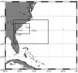
Figure 2.8. The setup of nesting domain. The outermost domain covers from 200 to 400 N and 850 to 600 W with resolution 12 minute. The mid domain is 280-350 N, 820-700W with 4 minute as the spatial grid size. The inner most domain is 310-340N, 81.50-76.50W with resolution 2 minute.

85oW 80oW 75oW 70oW 65oW 60oW

20oN

24oN

28oN

32oN

36oN

40oN

41002 Fpsn7 41004

(53)

(54)

0 5 10 15 SWH ( m )

a)Floyd SW H 41004(32.50N 79.10W )

BUOY Data Swan(Med) Swan(Inner) Swan(Outer) 0 2 4

6 b)Floyd SW H 41008(31.40N 80.87W )

SW

H

(

m

)

0 10 20 30 40 50 60 70 80 90 100

0 5 10

c)Floyd SW H Fpsn7(33.49N 77.59W )

Time (Hr) SW H ( m )

(55)

References

Battjes, J.A. and H.W., Groenendijk, 2000. Wave height distributions on shallow foreshores.

Coastal Eng. 40, 161-182.

Battjes, J.A. and M.J.F. Stive, 1985. Calibration and verification of a dissipation model for

random breaking waves. J.Geophys. Res. 90 (c5), 9159-9167.

Battjes, J.A., J., Janssen, 1978. Energy loss and set-up due to breaking of random waves.

Proc. 16th Int. Conf. Coastal Engg. ASCE, New York, pp. 569-587.

Berkhoff, J.C.W., 1972, Computation of combined refraction-diffraction. Proc. 13th Int.

Conf. Coastal Eng., ASCE 1, 471-490.

Booij, N., Ris, R.C., Hothuijsen, L.H., 1999. A third-generation wave model for coastal

regions: 1. Model description and validation. J. Geophys. Res. 104 (c4), 7649-7666.

Gao, Q., Radder, A.C., 1998. A refraction-diffraction model for irregular waves. Proc. 26th

Int. Conf. Coastal Eng. 1, 366-379.

Hasselmann, K., T.P. Barnett, E. Bouws, H. Carlson, D.E. Cartwright, K. Enke, J.A. Ewing,

(56)

Richter, W. Sell and H. Walden, 1973. Measurements of wind-wave growth and swell decay

during the Joint North Sea Wave Project (JONSWAP), Dtsch, Hydrogr.Z. Suppl., 12, A8.

Holland, G.J., 1980. An analytic Model of the wind and pressure profiles in Hurricanes.

Mon. Wea. Rev., 108, 121-1218.

Holthuijsen, L.H., A. Herman and N. Booij, 2003, Phase-decoupled refraction-diffraction for

spectral wave models, Coastal Engineering, 49, 291-305.

Hsu, T.-W., S.-H. Ou and J.-M. Liau, 2005, Hindcasting nearshore wind waves using a FEM

code for SWAN, Coastal Engineering, 52, 177-195.

Ito, Y., tanimoto, K., 1972, A method of numerical analysis of wave propagation-application

to wave diffraction and refraction. Proc. 13th Int. Conf. Coastal Eng., ASCE 1, 503-522.

Li, Y.S. and Zhan, J.M., 2001, Boussinesq-type model with boundary-fitted coordinate

system. J. Waterw., Port, Coast. Ocean Eng., ASCE, New York, 127 (3), 152-160.

Madsen, P.A. and Sørensen, O.R., 1992, A new form of the Boussinesq equations with

improved linear dispersion characteristics: Part2. A slowly-varying bathymetry. Coast. Eng.

(57)

Massel, S.R. and M.R. Gourlay, 2000. On the modeling of wave breaking and set-up on coral

reefs. Coastal Eng. 39, 1-27.

Ris, R.C., N. Booij and L.H. Holthuijsen, 1999, A third-generation wave model for coastal

regions, Part II, Verification, J.Geoph.Research C4, 104, 7667-7681.

Rogers, W.E., P.A. Hwang and D.W. Wang, 2003, Investigation of wave growth and decay

in the SWAN model: three regional-scale applications, J. Phys. Oceanogr., 33, 366-389.

SWAN group, 2003. SWAN Cycle III version 40.20 USER MANUAL.

Tolman, H.L., 1991, A third-generation model for wind waves on slowly varying, unsteady

and inhomogeneous depths and currents. J. Phys. Oceanogr., 21, 782-797.

Tolman, H.L., 2002. User manual and system documentation of WAVEWATCH-III version

2.22.

WAMDI group, 1998. The WAM model---a third generation ocean wave prediction model. J.

Phys. Oceanogr., 1775-1810.

Zhao Liuzhi, Vijay Panchang, W. Chen, Z. Demirbilek, N. Chhabbra, 2001. Simulation of

wave breaking effects in two-dimensional elliptic harbor wave models. Coastal Eng. 42,

(58)

Zijlema, M. and A.J. van der Westhuysen, 2005, On convergence behaviour and numerical

accuracy in stationary SWAN simulations of nearshore wind wave spectra, Coastal

(59)

CHAPTER 3. A NUMERICAL STUDY ON THE EFFECT OF

THE GULF STREAM ON WAVES

3.1.Introduction

The important and interesting fluid mechanical and environmental problem of the effect

of currents on waves has been the subject of significant community interested as reflected in

the many observing programs [e.g., Meadows et al., 1983; Mapp et al., 1985; Liu et al.,

1989] and theoretical studies [e.g., Treloar, 1986; Longuet-Higgins and Stewart, 1961;

Kengyon, 1971; Mathiesen, 1987]. Longuet-Higgins and Stewart [1960, 1961] developed the

theory of conserved wave-current interactions. They introduced radiation stress into the

governing equation. Kengyon [1971] investigated wave refraction in ocean currents by using

the geometrical optics approximation, and discussed the kinematical effects of currents on

waves. Mapp et al. [1985] developed a numerical model for the refraction of ocean swell by

current that was tested with Seasat synthetic aperture radar (SAR) data, in which integration

of the ray equation was applied in a moving medium. In 1987, Mathiesen developed another

model to study wave refraction by a current whirl, which extended the study of Mapp et al.

[1985]. Simons and Maciver [1998] performed experiments with regular deep-water waves

propagating obliquely across a relative narrow jet-type current.

The results of previous studies of current induced changes in wave height and direction

(60)

Stream) could be significant. In particular, the trapping of waves in currents and the total

reflection of waves by currents is theoretically possible. Irvine and Tilley [1988] discussed

the trapping of waves by straight and meandering shear currents. Holthuijsen and Tolman

[1991] investigated the effects of the Gulf Stream on surface gravity waves by employing the

WAVEWATCH wave model. Ocean waves were propagated across a current ring and as

well as across an infinitely long and straight northward flowing Gulf Stream from the

northeast (NE) and southeast (SE) directions. The results showed that refraction may trap

locally generated waves in the straight Gulf Stream or it may reflect wave energy back to the

open ocean depend on wind and wave conditions. However, in their research paper, they

didn’t investigate the condition of waves crossing the Gulf Stream from the normal direction.

The Simulating WAves Nearshore, or SWAN [Booij et al., 1999] a wave model that

includes depth induced dissipation and other sophisticated physics has been extensively

studied [Padilla-Hernandez and Monbaliu, 2001; Rogers et al., 2003; Holthuijsen et al., 2003;

Hsu et al., 2005]. However few studies have been focused on investigating the effects of

major currents on waves by employing SWAN. In the study of this chapter we repeat the

Holthuijsen and Tolman [1991] experiment but we use SWAN and we also investigate the

case of normal encounter of the wave field with the Gulf Stream as well as consider the case

of the Hurricane Bonnie induced wave field with an idealized Gulf Stream.

A brief outline of model setups and ideal experiments conducted in this chapter are given

in section 3.2. Section 3.3 presents the results of the ideal experiments to analyze the

(61)

introduced in Section 3.4. The comparison between model results and observation data for

the case of Bonnie is given in section 3.5. The last section in this chapter presents the

summary and discussion.

3.2.Setups of wave model and experiments

The computational domain is from 850 to 700 (W) longitudes and from 250 to 350 (N)

latitude with grid resolution 0.20. The water depth is set to 5000 m in order to avoid wave

refraction due to topography. The integration time step is 6 minutes. Wave frequencies range

from 0.04177 to 1.0 Hz and the directional resolution is 10° (00~3600). The current fields

(Gulf Stream) used in ideal experiments of this paper were simulated by X. Liu (personal

communication) using the HYbrid Coordinate Ocean Model, or HYCOM ocean current

model results published in Xie et al. [2006]. In Liu’s study, the Gulf Stream current fields

were simulated in the presence of climatological wind fields (COADS). The Gulf Stream

current field varies slowly in time and the result of the 51st day of the run is selected and

treated constant in time. Figure 3.1a shows the Gulf Stream current field of Day 51 from

Liu’s study.

In order to examine the influence of the Gulf Stream on waves, six ideal experiments

(Table 3.1) are conducted in this chapter. Locally generated wind waves and waves

propagating in as swell propagating in a direction counter to the direction of current

constitute cases NEW and NES. The cases SEW and SES are wind waves and swell

(62)

encountering the Gulf Stream from the east are investigated in the cases EW and ES.

Homogeneous and constant wind fields (10 m/s) were set as the wind input term of SWAN in

all of wind waves cases (NEW, SEW and EW). Three directions of the wind fields were

selected: one the NE wind (2250) (case NEW); the SE wind (1350) (case SEW); and the E

wind (1800) (case EW). The set up of the wave swell cases for SWAN are as follows: the

boundary condition is characterized with a Gaussian-shaped frequency energy spectrum; the

width of the Gaussian frequency spectrum is 0.007 Hz; the significant wave height is taken as

1.99 m; peak frequency is 0.071 Hz; peak wave directions are 2250 (NES), 1350 (SES) and

1800 (ES); and the directional width is 12.40. All angles used in this paper assume a Cartesian

convention.

3.3.Results

A single line (Fig. 3.1a) traversing the Gulf Stream was set to sample the wave character

parameters to show the variation in wave fields. The line is from 80.60W to 79.40W

longitudes and the latitude is 30.20_{N. The profile of the current speed (y direction) along this}

line is shown in Fig. 3.1b.

3.3.1．Case NEW

First we consider the results under the NE wind condition. Figure 3.2a shows the

Analysis and Modeling of Wave-current Interaction

Analysis and modeling of wave-current interaction

Huiqing Liu

Marine, Earth and Atmospheric Sciences

DEDICATION

BIOGRAPHY

ACKNOWLEDGMENTS

TABLE OF CONTENTS

LIST OF TABLES

LIST OF FIGURES

CHAPTER 1. INTRODUCTION

CHAPTER 2. INVESTIGATION OF DEPTH-INDUCED

REFRACTION-DIFFRACTION, WAVE BREAKING AND

NESTING IMPACTS ON WAVES USING SWAN

CHAPTER 3. A NUMERICAL STUDY ON THE EFFECT OF

THE GULF STREAM ON WAVES