ABSTRACT
ALTUNTAS, ALPER. An Adaptive Multi-Analysis Technique and Software Architecture for Ocean Circulation Models. (Under the direction of Dr. John Baugh.)
Hydrodynamic models are widely used by scientists and engineers to assess the impacts of coastal hazards such as tides, hurricane storm surge, and wind waves. These models require a substantial amount of computational resources due to the geographical extent of coastal pro-cesses and complex nature of ocean physics. When multiple what-if scenarios are to be evaluated, either as part of a forecasting/hindcasting study or a sensitivity analysis, the computational demand further increases.
This dissertation presents an adaptive multi-analysis technique to increase the computa-tional efficiency of ocean models when multiple local scenarios are to be evaluated. The tech-nique, calledadaptive subdomain modeling, is realized by the concurrent execution of multiple child domains, each corresponding to a local scenario, and a full-scale parent domain providing the boundary conditions for the child domains. During runtime, the spatial extent of each child domain is adaptively adjusted depending on the movement of altered hydrodynamics, i.e., the differences between the solutions of the child domain and the parent domain, to maintain both the efficiency and the reliability.
In addition to the adaptive subdomain modeling approach, the study includes the develop-ment of a generic software architecture for numerical ocean models, based on object oriented design principles and data abstraction. The new architecture utilizes concurrent executions of multiple domain instances and facilitates adaptive behavior. To demonstrate the effectiveness and applicability of the software architecture, we develop a simple finite-volume shallow water model and re-implement ADCIRC, an advanced finite-element ocean circulation model, with the incorporation of the adaptive subdomain modeling approach.
© Copyright 2016 by Alper Altuntas
An Adaptive Multi-Analysis Technique and Software Architecture for Ocean Circulation Models
by Alper Altuntas
A dissertation submitted to the Graduate Faculty of North Carolina State University
in partial fulfillment of the requirements for the Degree of
Doctor of Philosophy
Civil Engineering
Raleigh, North Carolina
2016
APPROVED BY:
Dr. Joel Dietrich Dr. Gnanamanikam Mahinthakumar
Dr. Alina Chertock Dr. John Baugh
DEDICATION
BIOGRAPHY
ACKNOWLEDGEMENTS
TABLE OF CONTENTS
LIST OF TABLES . . . vii
LIST OF FIGURES . . . .viii
Chapter 1 Introduction . . . 1
Chapter 2 Adaptive Subdomain Modeling: A Multi-Analysis Technique for Ocean Circulation Models . . . 5
2.1 Introduction . . . 6
2.2 Background . . . 8
2.2.1 ADCIRC . . . 8
2.2.2 Conventional subdomain modeling and applications . . . 9
2.3 Adaptive subdomain modeling . . . 12
2.3.1 Error indicator . . . 12
2.3.2 Adaptivity algorithm . . . 15
2.3.3 Boundary conditions . . . 26
2.4 Workflow and hybrid approach . . . 27
2.5 Test cases . . . 28
2.5.1 ASM control parameters . . . 29
2.5.2 Applications and Performance . . . 49
2.6 Conclusions and future work . . . 54
Chapter 3 A Generic Software Architecture for Concurrent and Adaptive Ocean Models . . . 57
3.1 Introduction . . . 57
3.2 Background . . . 59
3.2.1 Data Abstraction and OOP . . . 59
3.2.2 ASMFV Formulation . . . 61
3.2.3 ADCIRC Background . . . 63
3.2.4 Adaptive Subdomain Modeling . . . 64
3.3 Related Work . . . 66
3.4 The Architecture . . . 68
3.4.1 OpenHDM . . . 69
3.4.2 Inter-Domain Concurrency . . . 74
3.5 ASMFV . . . 77
3.6 ADCIRC++ . . . 79
3.6.1 Derived classes of ADCIRC++ . . . 80
3.6.2 Application of ASM in ADCIRC++ . . . 83
3.6.3 A case study: Hurricane Irene (2011) storm surge . . . 84
3.6.4 Discussion . . . 85
Chapter 4 Model Checking Wetting and Drying Algorithms . . . 89
4.1 Introduction . . . 89
4.2 Motivation . . . 92
4.3 Background . . . 94
4.3.1 ADCIRC Background . . . 94
4.3.2 Subdomain Modeling . . . 96
4.3.3 SPIN and Promela . . . 99
4.4 Abstracting Wetting and Drying Algorithms . . . 106
4.4.1 Discretization in Space and Time . . . 106
4.4.2 Data and Control Flow . . . 108
4.5 Case Study: ADCIRC’s wetting and drying algorithm . . . 109
4.5.1 Abstract Grid . . . 110
4.5.2 Control Flow . . . 112
4.5.3 Elemental drying with three wet nodes . . . 117
4.5.4 Verification of wetting and drying in subdomains . . . 119
4.6 Limitations . . . 124
4.7 Related Work . . . 128
4.8 Conclusions . . . 128
BIBLIOGRAPHY . . . .130
APPENDICES . . . .142
Appendix A ADCIRC++ Input File Formats . . . 143
LIST OF TABLES
Table 2.1 Comparison of computational costs for Case 5. . . 53 Table 2.2 Comparison of computational costs for Case 6. . . 54
Table A.1 Format of ADCIRC++ project input file, where header is an alphanumeric description of the input file,projectIDis an alphanumeric id for the project,
nd is the number of domains, domainIDi, configDiri, and outputPathi are the domain id, configuration file directory, and path to the output files of the i.th domain, respectively, andparentIDi is the id of the parent domain ofi.th domain. (If the domain i is a parent domain, the fourth column in line 3 +i is left blank. . . 143 Table A.2 Format of ADCIRC++ domain configuration file, whereheaderis an
alphanu-meric description of the input file, domainType is the type of the domain (=“ADCIRC” for ADCIRC domains), typei is the type of the i.th input file (=14 for grid files, =15 for model configuration files, etc.), formati is the for-mat of thei.th input file (=“ADCIRC” for ADCIRC domains),fileDiri is the directory of the i.th input file relative to the directory of the configuration file. 143 Table A.3 Format of ADCIRC++.dif file, wherenp is the number of properties to be
locally modified, propertyIDi is the id of i.th property to be modified (e.g., “bathymetry”, “mannings n at sea floor”, etc.), nni is the number of nodes with modified propertyIDi, ni,j and vali,j are the node number and the new value of the modified property i of the j.th node in the set of nodes with modified propertyIDi. . . 144 Table A.4 Format of optional ADCIRC++ .asm file, where header is an alphanumeric
description of the input file, tau is the tolerance, sigma is the safety factor,
LIST OF FIGURES
Figure 2.1 Expansion and contraction of a locally modified Shinnecock Inlet child
do-main patch at various timesteps. . . 8
Figure 2.2 Subdomain extraction with the SMT user interface. . . 11
Figure 2.3 Flowchart of the modified timestepping loop for adaptive subdomain mod-eling (ASM steps shaded, steps common to ASM and CSM patterned, and original steps left unshaded). . . 13
Figure 2.4 Initial patch of the modified Shinnecock child domain. . . 16
Figure 2.5 Relationship between tolerance and error indicator during a simulation. The patch expands at timestepst1,t3, and t4, and contracts at timestept2 since ρmax falls beneathστ0. . . 17
Figure 2.6 Summary of criteria for expanding a patch. . . 19
Figure 2.7 Illustration of criteria for expanding a patch. . . 19
Figure 2.8 Summary of criteria for contracting a patch. . . 20
Figure 2.9 Illustration of criteria for contracting a patch. . . 21
Figure 2.10 Expansion stage of the adaptivity algorithm. . . 22
Figure 2.11 Main steps of the expansion of a child domain patch, where the patch bound-ary noder is marked for expansion at the first step of the algorithm. . . 23
Figure 2.12 Contraction stage of the adaptivity algorithm. . . 24
Figure 2.13 Main steps of the contraction of a child domain patch, where the patch boundary noder is marked for contraction at the first step of the algorithm. 25 Figure 2.14 The complete workflow of a typical ADCIRC++ run with ASM. . . 28
Figure 2.15 Case 1: Local change near Shinnecock Inlet. . . 30
Figure 2.16 Case 1: Progression of a Shinnecock child domain patch for τ0 = 10−3, σ = 10−2,λ= 10−4, andθ= 10, with elements in the patch darkened. Snapshots: (a) initial extent, (b) expansion at timestep 812, (c) largest patch (occurring at timestep 2 949), and (d) final extent (timestep 71 276). . . 31
Figure 2.17 Case 1:l2-norms of maximum elevation errors in Shinnecock child domains. . 32
Figure 2.18 Case 1: max-norms of maximum elevation errors in Shinnecock child domains. 33 Figure 2.19 Case 1: Average percentage of active elements in Shinnecock child domains (with λ,τ axes reversed). . . 34
Figure 2.20 Case 2: Local change at Hatteras Inlet. . . 35
Figure 2.21 Case 2: Progression of a Hatteras child domain patch forτ0 = 10−3,σ= 10−2, λ= 5×10⁻⁴, andθ= 100, with elements in the patch darkened. Shapshots: (a) initial extent, (b) expansion at timestep 1 905, (c) largest patch, and (d) final extent (timestep 691 196). . . 36
Figure 2.22 Case 2:l2-norms of maximum elevation errors in Hatteras child domains. . . 36
Figure 2.23 Case 2: max-norms of maximum elevation errors in Hatteras child domains. . 38
Figure 2.24 Case 2: Average percentage of active elements in Hatteras child domains. . . 38
Figure 2.26 Case 3: Progression of a Walden Creek child domain patch for τ0 = 10−5, σ = 10−2, λ= 5×10⁻⁴, and θ = 10, with elements in the patch darkened.
Snapshots: (a) initial extent, (b) extent at timestep 546 520, (c) largest extent
(occurring at timestep 570 694), and (d) final extent (timestep 668 367). . . . 40
Figure 2.27 Case 3:l2-norms of maximum elevation errors in Walden Creek child domains. 41 Figure 2.28 Case 3: max-norms of maximum elevation errors in Walden Creek child do-mains. . . 42
Figure 2.29 Case 3: Average percentage of active elements in Walden Creek child domains (with λ,τ axes reversed). . . 43
Figure 2.30 Case 4: Local change at Brunswick intake canal in the refined Cape Fear subdomain. . . 44
Figure 2.31 Case 4: Progression of a Brunswick child domain patch for τ0 = 10−3, σ = 10−1, λ = 10−5, and θ = 100, with elements in the patch darkened. Snapshots: (a) initial extent, (b) extent at timestep 1 098 072, (c) largest extent (occurring at timestep 1 203 758), (d) final extent (timestep 1 374 294). 45 Figure 2.32 Case 4:l2-norms of maximum elevation errors in Brunswick child domains. . 46
Figure 2.33 Case 4: max-norms of maximum elevation errors in Brunswick child domains. 47 Figure 2.34 Case 4: Average percentage of active elements in Brunswick child domains (with λ,τ axes reversed). . . 48
Figure 2.35 Case 5: Recording stations at the intake canal. . . 50
Figure 2.36 Case 5: Water surface elevations at intake canal recording stations for varying depths and Manning’s n values. . . 51
Figure 2.37 Case 6: Local changes on the Cape Fear River. . . 52
Figure 2.38 Case 6: Recording stations along the river bank. . . 52
Figure 2.39 Case 6: Velocities at recording stations for varying elevation raises and Man-ning’s n values. . . 53
Figure 3.1 Expansion and contraction of locally modified Shinnecock Inlet child domain patch at various timesteps. (Elements included in the patch are highlighted in darker colors.) [3] . . . 65
Figure 3.2 The simplified class diagram of OpenHDM . . . 70
Figure 3.3 Main function of ADCIRC++ . . . 71
Figure 3.4 Phase execution criteria for parents and children . . . 75
Figure 3.5 State diagram of the composition of a parent domain and a child domain with two phases. (Actions with prefixes pr and ch correspond to the ones engaged by the parent and the child, respectively. The indices shown between square brackets show the phase index for the specified domain. The action notify which follows the action runis subjected to hiding operator for brevity.) . . . 76
Figure 3.6 Flowchart of the timestepping loop of ADCIRC++ domains. . . 77
Figure 3.7 Class diagram of ADCIRC++. (All classes are derived from the generic code, except NodalAttr and Wind. Specialized input and output classes are not included.) . . . 80
Figure 3.9 ADCGrid class inherited from Grid template. (Attribute accessors and data
members are omitted for brevity.) . . . 82
Figure 3.10 The subdomain used as the parent domain and the deepened intake canal for Hurricane Irene simulation . . . 85
Figure 3.11 Progression of Irene child domain patch for τ = 10−3, σ = 10−1, λ=10−5, θ= 100. Elements included in the patches are highlighted in darker colors. (a) Initial extent. (b) Extent at timestep 1,098,072. (c) Largest extent (occuring at timestep 1,203,758) (d) final extent (reached at timestep 1,374,294) . . . . 86
Figure 4.1 A typical unstructured triangular finite element mesh used in hurricane storm surge modeling, that covers the Western North Atlantic with 620,089 nodes and 1,224,714 elements. . . 91
Figure 4.2 Subdomain Modeling Tool (SMT) user interface. . . 98
Figure 4.3 Wetting and drying data dependencies [12]. . . 99
Figure 4.4 A global variable, a SPIN process, and a safety property. . . 101
Figure 4.5 Concurrent incrementation. . . 101
Figure 4.6 Synchronized incrementation. . . 102
Figure 4.7 Synchronized incrementation with a selective structure. . . 103
Figure 4.8 A busy-wait implementation using a repetitive statement. . . 103
Figure 4.9 A message channel used as a lock. . . 104
Figure 4.10 Conditions for an abstract grid to represent a subset of any possible grid. . . 107
Figure 4.11 Determining the size of the abstract grid. . . 110
Figure 4.12 Abstract grids with minimum and maximum number of interface nodes. In-ternal and interface nodes are shown in red and gray, respectively. . . 111
Figure 4.13 Compound data types:Node,Element,Domain. . . 112
Figure 4.14 Macros to retrieve incident nodes of elementi. . . 112
Figure 4.15 Timestep initialization routine. . . 113
Figure 4.16 SPIN model of the first stage of the wetting and drying algorithm. . . 113
Figure 4.17 SPIN model of the second stage of the wetting and drying algorithm. . . 114
Figure 4.18 SPIN model of the third stage of the wetting and drying algorithm. . . 115
Figure 4.19 SPIN model of the fourth stage of the wetting and drying algorithm. . . 116
Figure 4.20 Updating permanent wet/dry states of nodes. . . 117
Figure 4.21 An inline asserting that elements with three wet nodes must be wet. . . 118
Figure 4.22 The initial process of elemental drying verification. . . 118
Figure 4.23 The guided simulation of the execution trail that results in the assertion violation. . . 119
Figure 4.24 An example configuration for abstract full domain and subdomain grids. . . . 120
Figure 4.25 The declarations of the boundary conditions channel and inlines. . . 121
Figure 4.26 A mechanism for non-deterministic choice synchronization. . . 122
Figure 4.27 The modified inline of the third part of the algorithm. . . 122
Figure 4.28 The modified nodal loop inpart4(domain). . . 123
Figure 4.30 The shortest path to the counterexample found in absence of intermediate forcing. (The trail includes additional printf statements for further clarifica-tion.) . . . 126 Figure 4.31 Progression of wet/dry states of nodes and elements in absence of
intermedi-ate wet/dry forcings for the subdomain. Dry nodes and elements are shown in yellow, while wet nodes and elements are shown in blue. Inactive elements are either dry or has at least one dry node. . . 127
Chapter 1
Introduction
Hurricane storm surge poses a substantial threat to the built and natural environment in coastal communities. While the devastating impacts of the surge events in recent years, such as the ones induced by Hurricane Katrina (2005) and Hurricane Sandy (2012), remind us of the value of disaster preparedness and risk mitigation efforts, studies on the effects of climate change and sea level rise indicate an increasing risk associated with coastal hazards in the future [73, 89]. In addition to climatic factors, population growth and increasing urbanization in low-lying regions further escalate the vulnerability to inundation [52]. Thus, the prediction and analysis of coastal hazards are highly critical for creating more resilient coastal communities.
Given the spatial and temporal extent of coastal events and complex nature of ocean physics, numerical ocean models require a substantial amount of computational resources. When mul-tiple what-if scenarios are to be evaluated, whether as part of forecasting/hindcasting studies or sensitivity analyses, computational demand further increases, since regardless of the extent of the alterations, each design scenario requires a large-scale simulation to fully capture the physics of coastal processes.
This study presents an adaptive multi-analysis technique for ocean models to reduce the computational effort when multiple local changes are to be evaluated. The technique, called adaptive subdomain modeling, is realized by the concurrent analysis of any number of child domains, each corresponding to a unique design and failure scenario, and an original full-scale parent domain. Based on a prior subdomain modeling approach with static boundary locations, the new approach eliminates the requirement for users to determine the sizes and shapes of modified domains extracted from an original full-scale domain: the spatial extent of each child domain is automatically initialized to cover only the modified regions and is adaptively adjusted during runtime depending on the movement of altered hydrodynamics, i.e., the differences between the solutions of a child domain and its parent domain, originating from the local changes. At every timestep, an error measure indicative of the differences between the solutions of a child domain and its parent domain is calculated around the boundaries to assess the proximity of altered hydrodynamics. If the error indicator is determined to be greater than a user-specified tolerance, then the boundary is moved outward to ensure that the boundary conditions obtained from the concurrent parent domain remain valid. If the error indicator is sufficiently small, then the boundary is moved inward to reduce the computational effort. Thus, the approach ensures that child domain simulations are always accurate and efficient.
incorporation of new features. Our software architecture, however, is based on object oriented programming principles that enhance modularity, maintainability, and extensibility through data abstraction and encapsulation. The architecture, consisting of two levels of source code, facilitates adaptive behavior and utilizes concurrent executions of multiple domain instances. The first level source code is a generic framework consisting of class templates and abstract classes that can accommodate ocean models with different numerical methods and formula-tions, and the second level is implementation-specific source code that is specialized for the details of the model to be developed. The generic framework also includes a shared-memory parallel implementation for the concurrent execution of multiple domain instances. We demon-strate the effectiveness and flexibility of the architecture by modeling a simple finite-volume shallow water equation solver and by re-implementing ADCIRC, an advanced finite-element ocean circulation model. We incorporate the adaptive subdomain modeling approach in the new implementation, called ADCIRC++, and discuss the advantages of object oriented design in terms of maintainability, extensibility, and computational efficiency.
While object oriented software design facilitates the addition of new computational tech-niques, the correctness of the algorithmic behavior of an ocean model still needs to be verified for newly acquired features. As an alternative to testing and deductive reasoning, this study proposes the application of model checking tools for the formal verification of algorithmic model behavior. Mainly used for the verification of concurrent hardware and software systems, model checkers analyze the abstract representations of actual systems, which are generated by the users as inputs, and guarantee an effective verification procedure due to their exhaustive state-space exploration strategy. To demonstrate the applicability, the wetting and drying algorithm of ADCIRC is modeled using the SPIN model checker, and the correctness of the algorithm for adaptive subdomain modeling is verified.
Chapter 2
Adaptive Subdomain Modeling: A Multi-Analysis
Technique for Ocean Circulation Models
2.1
Introduction
A comprehensive evaluation of the damaging effects of coastal hazards on the built and natural environment requires the assessment of many potential model configurations. While modifica-tions corresponding to design and failure scenarios are often local in nature, ocean processes such as tides and hurricanes operate over significantly larger scales. As a result, despite the limited geographic extent of a region of interest, each local configuration requires a large-scale simulation to accurately capture the physics of the hydrodynamic processes involved [19].
To address this difference in scale, a prior study presented an exact reanalysis technique, called subdomain modeling, that enables the assessment of multiple local changes without requiring a separate full-scale simulation for each one [12]. The technique, implemented in ADCIRC, introduces a new boundary condition type that combines water surface elevation, velocity, and wet/dry status. The workflow begins with the extraction of subdomains from an original full-scale domain. Once subdomain grids are generated, a full-scale simulation is performed to obtain boundary conditions for each subdomain. Local changes corresponding to design and failure scenarios can then be applied to subdomain grids, provided the altered hydrodynamics remain within the boundaries, which are forced with data obtained from the original configuration. The technique substantially reduces the computational effort required to analyze local changes, but requires that users determinea priori the size and shape of each subdomain by anticipating the spatial extent of the effects of those changes. The efficiency of the technique may be reduced when subdomains are oversized, whereas, if undersized, the entire exercise may need to be repeated.
In this study, we present an adaptive subdomain modeling (ASM) technique where the sizes and shapes of computationally active regions, called patches,1 of locally modified grids are automatically determined and adaptively adjusted during runtime. The technique is real-1The termpatch has a variety of definitions depending on context. For instance, in GeoClaw, a finite-volume
ized by concurrently executing the simulations of multiple child domains, with each instance corresponding to a local scenario, and a full-scale parent domain providing the boundary con-ditions for the child domains. Initially encompassing only the modified regions, the patches of child domains are dynamically adjusted during runtime depending on the response of the model. An error indicator—a measure of the difference between the solutions of the parent and child domains—is calculated near the boundaries of patches to assess the proximity of altered hydrodynamics to the boundaries. In case the error indicator is determined to be larger than a user-specified tolerance, the patch boundary at that location is moved outward to ensure that the changing hydrodynamics approaching the boundary do not reach it before the next timestep. If the error indicator is determined to be sufficiently small, on the other hand, the patch is contracted to increase computational efficiency. An example of a child domain as a dynamically adjusting patch is shown in Fig. 3.1.
To accommodate the ASM approach, we make use of a re-implementation of ADCIRC with an updated software architecture that more readily supports adaptivity. In its original form, ADCIRC is based on procedural decomposition, with code that is structured by dividing control flow into subroutines, and where the primary data structures are global and non-reentrant. Our new architecture, on the other hand, is based on data abstraction, where the internal repre-sentation of a data type is distinct from its external view. This style of programming enhances modularity, maintainability, and extensibility by ensuring that the changes made within a data structure do not propagate to the rest of the program [13]. The new implementation, called ADCIRC++, facilitates adaptive grid behavior and utilizes concurrent executions of multiple domains by means of dynamic containers and object-oriented design principles [4].
Figure 2.1: Expansion and contraction of a locally modified Shinnecock Inlet child domain patch at various timesteps.
and CSM workflows and a hybrid approach that combines the two. Section 2.5 includes para-metric studies with test cases that serve as a guide for determining the ASM control parameter settings subsequently used, and a sensitivity analysis that demonstrates the applicability and computational efficiency of the method. Finally, conclusions and future work are presented.
2.2
Background
2.2.1 ADCIRC
Combined with the flexibility of unstructured triangular meshes, ADCIRC’s formulation of the governing equations and optimized numerical algorithms constitute an efficient and versatile modeling system [74].
As for the computational process, at every timestep ADCIRC solves the generalized wave continuity equation (GWCE) to obtain water surface elevations, then executes a wetting and drying algorithm to determine the geographic extent of hydrodynamic activity, and finally solves the momentum equations to obtain velocities in thex and y directions.
ADCIRC simulations can be performed as three dimensional or two dimensional depth integrated (2DDI) analyses. The linear system of the GWCE can be configured so that it is based on either consistent or lumped mass matrices, and time discretization may be performed either implicitly or explicitly. The consistent GWCE system is solved using an iterative Jacobi conjugate gradient method. For a 2DDI model with a consistent matrix solver and implicit timestepping scheme—as used in this study—both the GWCE and the momentum equations are discretized in space using the Galerkin finite element method [90], and the GWCE is discretized in time using a variably weighted three-time-level implicit scheme for the linear terms, while the momentum equations are discretized in time using a two-time-level implicit Crank-Nicolson approximation [74].
2.2.2 Conventional subdomain modeling and applications
The CSM workflow is as follows:
1. Construct a subdomain
1.1. Locate one or more regions of interest within the original full domain
1.2. Perform a simulation on the full domain to generate boundary conditions for each subdomain
1.3. Preprocess boundary condition files
1.4. Perform simulations on subdomains as a verification step
2. Generate engineering scenarios
2.1. Alter subdomains to realize engineering design and failure scenarios of interest
2.2. Perform simulations on altered subdomains
2.3. Check results of altered subdomains as a second verification step
The two verification steps in the workflow are performed to confirm that results from un-altered subdomains match their full domain counterparts, and that the new hydrodynamics induced by altered subdomains do not propagate to subdomain boundaries.
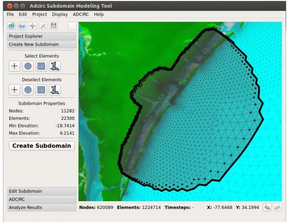
The pre- and post-processing steps of CSM are facilitated by a graphical user interface called SMT, the Subdomain Modeling Tool [42]. Multiple subdomains can be visually extracted using a variety of selection tools, as shown in Fig. 2.2. Once subdomains are defined by the user, the tool automatically generates the required input files for both the subdomains and the full domain.
Figure 2.2: Subdomain extraction with the SMT user interface.
Manning’s n fields are determined probabilistically, the results can then be used for predictive simulations, which may easily become computationally prohibitive. They point out, however, that the use of subdomain modeling can reduce the computational time and allow focusing on specific regions of interest that are prone to hurricane storm surge. Subsequently, Graham, one of the co-authors, reduces the cost of a series of forward models using the subdomain modeling approach for his Hurricane Gustav Case Study [47], where he extracts a subdomain grid with 15 001 elements from a full-scale grid consisting of 2 720 591 elements. He notes that the runtime required for the full-scale grid is about 3 300 CPU-hours, whereas for the subdomains it is only 11 CPU-hours.
sensitivity studies require substantial computational resources, they remark on the anticipated value of subdomain modeling in reducing the cost of repeated simulations with adjustments to the grid and the vegetation parameters in the regions of interest.
2.3
Adaptive subdomain modeling
ASM is an improved and complementary technique for ocean models that allows the simulation of locally modified child domains to be performed concurrently. Such modifications, for in-stance, might include changes to bathymetry, bottom friction, and elemental slope limiters that constitute an alternative modeling scenario. By adaptively moving boundaries that are forced with data from the parent, the technique avoids performing computations that are external to a child domain and therefore redundant.
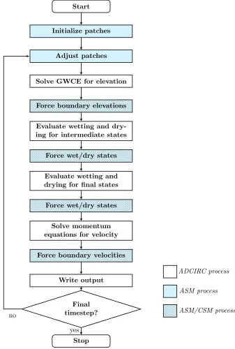
The ASM approach consists of three essential components. First, an error indicator de-termines the progression of altered hydrodynamics. Second, an adaptivity algorithm for the expansion and contraction of patches manages the insertion and removal of nodes and el-ements. Finally, boundary conditions are prescribed for accurate computations within child domain patches. In our implementation, the original ADCIRC timestepping loop is modified so that the adaptivity algorithm is executed at the beginning of each timestep to determine and apply any necessary adjustments to patch boundaries. Then, boundary conditions are en-forced at specified control points as is done in the CSM approach. A flowchart of the modified timestepping loop for ASM is shown in Fig. 2.3.
2.3.1 Error indicator
Start
Initialize patches
Adjust patches
Solve GWCE for elevation
Force boundary elevations
Evaluate wetting and dry-ing for intermediate states
Force wet/dry states
Evaluate wetting and drying for final states
Force wet/dry states
Solve momentum equations for velocity
Force boundary velocities
Write output
Final timestep?
Stop
ADCIRC process
ASM process
ASM/CSM process
yes no
timestep++
efficiency. Such indicators may be based on solutions [14, 43, 66], derivatives of solutions [72, 91], mass residuals [91, 36, 78], or truncation errors [16, 18]. Thus, their purpose is to guide decisions about mesh refinement and corresponding numerical schemes in an effort to improve overall convergence. In ASM, by way of contrast, the objective is to detect the altered hydrodynamics originating from local changes, and thereby ensure that each locally modified child domain behaves as though it were part of its own full-scale domain in a full-scale simulation. As a result, an error indicator based on differences between the solutions of child domains and parent domains is chosen:
ρ=max(ρη, ρu, ρv) (2.1)
where
ρη =
|ηchild−ηparent| p
0.5(|ηchild|+|ηparent|) 2
ρu=
|uchild−uparent|
p
0.5(|uchild|+|uparent|) 2
∆t
ρv =
|
vchild−vparent| p
0.5(|vchild|+|vparent|) 2
∆t
η: water surface elevation
u:x velocity
v:y velocity
∆t: step size in seconds
com-pared with the error indicators of the adjacent nodes to determine whether the patch boundary should be moved at that location.
2.3.2 Adaptivity algorithm
In the ASM approach, child domain patches are first initialized to include only the nodes whose properties have been modified as part of an alternative modeling scenario, along with a three-layer buffer of surrounding nodes and elements, as shown in Fig. 2.4. Each three-layer has a rationale: the first is adjacent to and directly affected by changes to modified nodes, the second assesses the potential for altered hydrodynamics, and the third enforces boundary conditions obtained from the parent domain. Once the initial patch of nodes and elements has been determined and
activated for each child domain, the corresponding systems of equations are constructed, and simulation can begin. Then, during runtime, child domain patches are adaptively adjusted to ensure that they are just large enough to cover the altered hydrodynamics. Control parameters that determine the shapes and sizes of patches are as follows:
tolerance (τ): a parameter that varies with timestep and against which error indicators are compared to determine whether a patch expands; the comparison is of the formρ > τ. An initial tolerance of τ0 is set by the user, and subsequent changes are made as necessary by the adaptivity algorithm.
minimum activation interval (θ): the minimum number of timesteps throughout which a newly activated node must stay active; nodes within a patch are referred to asactive.
decay constant (λ): a parameter controlling the exponential decay of toleranceτ based on a reduction of the form e−λ. Such reductions are applied after an increase in tolerance to return it over time to its initial setting,τ0.
contraction factor (σ): a constant set by the user that, along with the initial toleranceτ0, is
Figure 2.4: Initial patch of the modified Shinnecock child domain.
As an illustration of the relationship between control parameters, Fig. 2.5 shows a time history of the maximum error indicator at a timestep and its effect on the maximum tolerance for a hypothetical child domain. Each time the tolerance is exceeded by the error indicator near a patch boundary, the boundary is moved outward one layer, and the tolerance of the newly expanded boundary node (e) is set to the sum of the initial tolerance and the error indicator value of the marked node (m) causing the expansion; in other words,τet+1=τ0 +ρtm. Increasing the tolerance affords local errors some time to decrease without causing the boundary to be moved outward repeatedly at consecutive timesteps. Locally increased tolerances return to their initial setting over time based on the user-specified exponential decay constant (λ).
Boundary expansion and numerical stability
Before elaborating on the stages of the adaptivity algorithm, we consider the relationship be-tween the boundary expansion procedure and the stability of the numerical scheme, which taken together must ensure that altered hydrodynamics are contained within the patches of child domains throughout the simulation.
condi-Figure 2.5: Relationship between tolerance and error indicator during a simulation. The patch expands at timestepst1,t3, and t4, and contracts at timestep t2 sinceρmax falls beneath στ0.
tion, which is necessary for the convergence of hyperbolic PDEs. The CFL condition states that a method can only be convergent if the numerical domain of dependence encompasses the ana-lytical domain of dependence of the PDE [69]. Since hyperbolic PDEs have a finite information propagation speed, their domain of dependence is finite, i.e., the solution at a node depends only on a finite domain [54]. The CFL condition is tested by comparing the Courant number, a ratio of ∆tto ∆x, against an upper bound. For ADCIRC and its semi-implicit time marching algorithm, the Courant number should be at most 0.5 for open ocean flows, and much less for other situations like near-shore flows with wetting and drying [40]. It is defined as:
Cr=
√
gh∆t
∆x (2.2)
In summary, the CFL condition limits the maximum stable step size for a computational grid so that the solution at any point does not propagate beyond the domain of dependence, i.e., one layer of elements, within a timestep. This restriction also ensures that expanding a child domain by a single layer of elements is sufficient to contain the altered hydrodynamics: such changes are guaranteed to propagate no further than a layer at a time, and therefore cannot reach the boundary. Once differences are detected at a node, the patch is expanded so thattwo layers separate any such nodes from the patch boundary.
As an alternative to the semi-implicit time-marching algorithm, one might consider using an implicit scheme so that the Courant stability constraint can be relaxed [41]. In ADCIRC, however, the wetting and drying algorithm imposes an additional restriction on step size, since wetting fronts can propagate only one layer per timestep [33]. As a result, regardless of the time-marching algorithm employed, the step size must be small enough so that the solution is limited to advancing a single layer of elements at a time, further justifying the ASM expansion policy in practice.
Stages of the adaptivity algorithm
The adaptivity algorithm consists of four main stages that are executed in turn at the beginning of each timestep. In the first, the algorithm calculates the error indicatorρ near patch bound-aries, marks areas where a tolerance is exceeded for expansion, and areas where the indicators are sufficiently small for contraction. In the remaining three stages it performs the expansions and contractions, and finally carries out a post-processing step to update the affected properties and data structures. Implementation details of each stage are given below.
nodes are marked for expansion in a subsequent stage. As patches grow, they may eventually coincide with certain types of boundaries defined in the parent domain, such as mainland or island boundaries. However, if they reach boundary types defined by flux or water surface el-evation, such as an open ocean boundary, execution of the child domain is aborted since it will have failed to satisfy the specified tolerance. The criteria for expansion are summarized in Fig. 2.6 and illustrated in Fig. 2.7.
Expansion criteria:mark a patch boundary nodeifor expansion if
• ∃n∈ineitab(i) :ρn> τi and
• inot adjacent to a grid boundary (except island or mainland) whereineitab(i) is the set of neighboring internal nodes of i.
Figure 2.6: Summary of criteria for expanding a patch.
For contraction, several criteria come into play. The first is that all internal neighbors of a patch boundary node must have error indicator values ρ less than στ0, the product of the contraction factor and the initial tolerance. Then, the same test must be satisfied by the neighbors’ neighbors of the boundary node, since nodes adjacent to the boundary node are about to become boundaries themselves (once the boundary node under consideration is deactivated). Continuing with other criteria, the minimum activation intervalθ must be satisfied to prevent flickering of the nodes and elements, as is done in AMR implementations [66]. Finally, the boundary node under consideration should not be adjacent to a node marked for expansion, and it should not be one of the initially active nodes in the original patch. If these hold, such nodes are marked for contraction in a subsequent stage and added to a deactivation list. The criteria for contraction are summarized in Fig. 2.8 and illustrated in Fig. 2.9.
Contraction criteria:mark a patch boundary nodeifor contraction if
• ∀n∈ineitab(i) :ρn< στ0 and ∀m∈ineitab(n) :ρm< στ0 and
• iactivated at least θtimesteps ago and
• inot adjacent to an expansion node and
• inot included in the initial patch
whereineitab(i) is the set of neighboring internal nodes of i.
Figure 2.8: Summary of criteria for contracting a patch.
Figure 2.9: Illustration of criteria for contracting a patch.
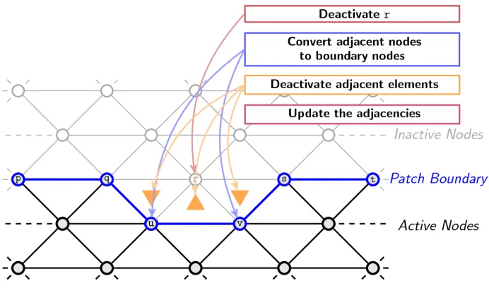
tolerances of new patch boundary nodes. Fig. 2.11 illustrates the approach.
With respect to memory management, optimizations are performed to minimize repetitive allocation and deallocation of nodes and elements. When a node external to a patch is activated for the first time, for instance, space is allocated for it as part of the child domain. The node is also marked as active, but at a later time it might be deactivated, at which point it is removed from the child domain but its underlying space allocation remains. If it is subsequently activated, then, no reallocation of space is required.
After the designated nodes and elements are activated, some bookkeeping and clean-up steps must be performed. The connectivity of all nodes and elements affected by the activations is updated. Patch boundary nodes not marked for expansion that are surrounded by newly activated nodes and elements are converted to internal nodes to prevent them from being treated as boundary conditions and checked for expansion or contraction. Finally, the tolerances of the new boundary nodes are updated.
Stage 2:Expansion Algorithm
• Let expansionNodes be the set of patch boundary nodes where the boundary is to be expanded. The set is assembled in Stage 1
• Let nodesToAllocateand nodesToActivatebe empty sets of nodes
• Let neighbors(i)be the set of nodes adjacent to node i • Let elements(i)be the set of elements incident on nodei • Let nodes(i)be the list of nodes of elementi
1: foriinexpansionNodes do
Convertito internal node .to remove it from the set of patch boundary nodes forjinneighbors(i) do
if jis not instantiated beforethen
nodesToAllocate.insert(j) . copy the external neighbor from parent grid else if jis inactivethen . (i.e., copied at a previous timestep)
nodesToActivate.insert(j)
2: foriinnodesToAllocatedo
Copy ifrom parent and insert to patch
if iis mainland boundary or island boundary then Update the relevant vectors and parameters 3: foriinnodesToActivatedo
Insert ito patch .and so activatei
Copy time-varying properties of nodeifrom parent 4: foriin(nodesToActivate+nodesToAllocate) do
forjinelements(i)do .loop through elements connected toi
if (j is not instantiated before)and (all three nodes of jare instantiated)then Copy jfrom parent
if (j is inactive)and (all three nodes of jare active)then
Insert jto patch .and so activatej
forkin nodes(j)do . loop through nodes of elementj
Updateelements(k)
5: foriin(nodesToActivate+nodesToAllocate) do Updateneighbors(i)
forjinneighbors(i) do Update neighbors(j)
6: foriin(nodesToActivate+nodesToAllocate) do if iis connected to at least one inactive node then
Convert ito boundary node
else . i.e., surrounded by active nodes
Convert ito internal node
Figure 2.11: Main steps of the expansion of a child domain patch, where the patch boundary node r is marked for expansion at the first step of the algorithm.
process that list by actually deactivating nodes in the child domain, and update the connectivity of nodes and elements. Fig. 2.13 illustrates the approach.
Before any nodes are deactivated, the algorithm checks for inconsistencies. As a result of the marking in stage 1, some of the patch boundary nodes may become disconnected from internal nodes and remain connected only to patch boundary nodes; such nodes are now added to the deactivation list. Conversely, some nodes are removed from the deactivation list, namely, those that are surrounded by active nodes as a result of expansions, and those that are adjacent to an expansion node or a recently activated node.
Stage 3:Contraction Algorithm
• Let contractionNodes be the set of patch boundary nodes where the boundary is to be contracted. This set is assembled in Stage 1
• Let patch.boundaryNodesbe the set of boundary nodes of patch • Let deactivatedElementsbe an empty set of elements
• Let neighbors(i)be the set of nodes adjacent to node i • Let elements(i)be the set of elements incident on nodei • Let nodes(i)be the list of nodes of elementi
1: foriinpatch.boundaryNodes do
if (i is connected only to patch boundary nodes)and (iis not initially active) then
contractionNodes.insert(i)
2: foriincontractionNodes do
if (i is not at the boundary anymore) or (iis next to an expansion node)
or (iis next to a recently activated node)then
contractionNodes.remove(i)
3: foriincontractionNodes do Deactivatei
Convert i to internal node .to remove it from the set of patch boundary nodes forjinneighbors(i) do
Update neighbors(j)
if (jis internal node) then Convertjto boundary node forkinelements(i)do
Deactivate k
deactivatedElements.insert(k)
for linnodes(k)do . loop through nodes of elementk
Updateelements(l)
4: foriindeactivatedElements do
if any node jof iis not connected to any active elementthen Deactivate j
Convert j to internal node .to remove it from the set of patch boundary nodes for kinneighbors(j) do
Updateneighbors(k)
if (kis internal node)then Convertkto boundary node if any two nodes of iare disconnected then
Update neighborsof both nodes
Figure 2.13: Main steps of the contraction of a child domain patch, where the patch boundary node r is marked for contraction at the first step of the algorithm.
Stage 4: Post-processing After the expansion and contraction processes are complete, prop-erties and containers of the child domains are updated in this final stage of the algorithm. As part of that process, the system of equations associated with any expanded or contracted patch is reset and resized. Then, auxiliary containers holding nodal data are updated. Finally, patch boundary nodes with tolerances greater thanτ0 are subjected to an exponential decay so that
their individual tolerances converge toward the initial tolerance over time. For a patch boundary node j at timestept, the tolerance is updated as follows:
τjt= (τjt−1−τ0)e−λ+τ0 (2.3)
2.3.3 Boundary conditions
To perform simulations concurrently, an interface is needed between a parent domain and its children. For its basis, we adapt the boundary condition type used in CSM, which incorporates water surface elevation, wet/dry status, and velocity, to realize a one-way hand off from parent to child [12]. The conventional approach to subdomain modeling obtains these quantities after completion of a full-scale run, and then applies them to static boundaries of a subdomain. In ASM, of course, boundaries are in motion, but only at the start of a timestep, giving us a static snapshot afterward in which boundary conditions may be applied. To do so, we (a) specify nodal elevations in the implicit GWCE formulation, (b) force wet/dry status on boundary nodes in the wetting and drying routine, and (c) assign boundary velocities outright in the momentum equation solver.
Of the three conditions—water surface elevation, wet/dry status, and velocity—the en-forcement of nodal wetting is somewhat less straightforward because, during each timestep, ADCIRC’s wetting and drying algorithm [37] performs several updates to a node before its final wet/dry state is set, and these intermittent changes are spatially dependent on the in-termediate states of other, neighboring nodes. In a prior study [12], we present an analysis of data dependencies and interactions between the wetting and drying algorithm and the hand off required by subdomain modeling and other mesh partitioning schemes. Included is a proof showing that, for correctness, the multipleintermediate wet/dry states of a subdomain bound-ary node can be set with a single value: the node’sfinal wet/dry state at a given timestep from a full run.2 The implication is that the only data transfer required from one domain to another is that of the final wet/dry states, simplifying communication between domains. Applying this result to ASM, we again note that patch boundary nodes are spatially adjusted at the beginning of a timestep and otherwise remain fixed throughout its execution. Thus, apart from extraction and processing procedures, boundary conditions in ASM can be enforced in the same manner as they are in CSM.
2
2.4
Workflow and hybrid approach
Using ASM begins with a modeling step: identifying geographic locations of interest and de-termining the alternatives to be simulated in concert with an ordinary ADCIRC model. Then, a single input file for each child domain is created: a difference file (.dif) containing a list of modified nodes along with new values of their associated properties, e.g., bathymetry, bottom friction, and elemental slope limiters. In contrast with CSM, subdomain boundaries are not defined, and the abbreviated versions of input files ordinarily used by subdomains are not re-quired. Instead, the locations, sizes, and shapes of initial child domain patches are determined automatically, and model parameters are copied as needed from the parent domain.
With respect to other input files, we rely on standard ADCIRC file formats and add some of our own. To organize them, we define the notion of a project to be an ordinary ADCIRC model plus some number of child domains: a project file (.prj) contains a list of the included domains, i.e., the parent and all of its children. Each domain included in a project file has an associated configuration file (.cfg) that points to the locations of standard ADCIRC files used by the domain and a difference file. An optional input file for child domains is the ASM file (.asm), where control parameters for adaptive subdomain modeling are set; if missing, default values are assumed.
In addition to being straightforward, the ASM workflow eliminates two verification steps that are required by CSM: confirming the stability of unaltered subdomain grids, and ensuring that altered hydrodynamics do not reach subdomain boundaries. Fig. 2.14 summarizes the complete workflow of a typical ADCIRC++ run with ASM.
0. Begin with an ordinary ADCIRC model
1. Generate ADCIRC++ input files:
• a difference file (.dif) with modified nodes for each child domain
• a project file (.prj) that lists parent and child domains
• a configuration file (.cfg) for each domain that points to standard ADCIRC files, a difference file, and an optional ASM file (.asm) 2. Run ADCIRC++
Figure 2.14: The complete workflow of a typical ADCIRC++ run with ASM.
While ASM offers some important advantages, an apparent weakness is the inability of users to alter one or more child domains after reviewing the results produced by another, unless they resort to running another full-scale simulation. However, ASM and CSM are complementary techniques that can be used in combination in cases such as the above, which call for a sequential analysis of subdomains. Using CSM, a single, full-scale simulation can produce one or more conventional, static subdomains, any of which can be used as the parent domain in an ASM simulation with any number of child domains. We refer to this combination ashybrid subdomain modeling (HSM), and present examples of its use below.
2.5
Test cases
In all cases, errors are determined by comparing ASM results with a separate, independent run of a parent domain that directly incorporates the local change previously simulated by its children.
2.5.1 ASM control parameters
For evaluating the effects of ASM control parameters on accuracy and efficiency, we look at the following four cases:
1. Shinnecock Inlet on the south shore of Long Island, NY
A tidal model with a coarse grid, limited area, and a bathymetric change in the inlet
2. Hatteras Inlet located along the Outer Banks, NC
A tidal model with a finer grid, spanning North Carolina, and a bathymetric change in the inlet
3. Walden Creek at Southport, NC
Hurricane Fran (1996) simulated on a subdomain around Cape Fear, with an added pro-tective structure
4. Brunswick intake canal at Southport, NC
Hurricane Irene (2011) simulated on a more refined subdomain around Cape Fear, with depth added all along the Brunswick nuclear power plant’s intake canal
Case 1: Shinnecock Inlet with tidal forcing
As an introductory example, a tidal model developed by the USACE Coastal Hydraulics Lab-oratory [80, 81, 95] and available on the ADCIRC website [2] is used. Centered on Shinnecock Inlet, New York, the model is realistic, though coarse in time and space, with a grid of 5 780 elements and 3 070 nodes covering a small area. The total duration of the simulation is 5 days, and the step size is 6 s. Tidal constituents M2, N2, S2, K1, and O1 are applied as tidal potential forcings and tidal boundary forcings. To simulate a small, local change, the bathymetric depths of three nodes near the inlet are reduced by 1 m, as shown in Fig. 2.15.
As the simulation unfolds, child domain patches with their local changes expand to contain the altered hydrodynamics. For ASM control parameter settings of τ0 = 10−3, σ = 10−2, λ = 10−4, and θ = 10, for instance, the associated patch reaches its maximum size of 910 elements (about 16% of the entire grid) at timestep 2 949 (about 4% of simulated time), as shown in Fig. 2.16. The size of the patch remains mostly the same throughout the simulation, since expansions and contractions come into equilibrium once it covers the maximum region of altered hydrodynamics.
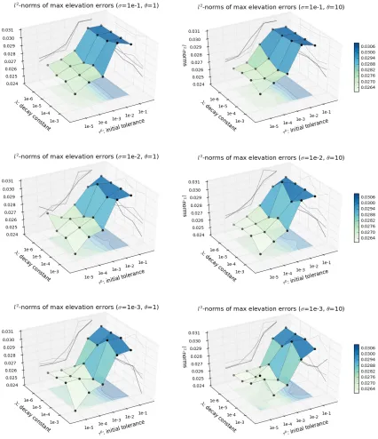
For the parametric study, 120 (= 5×3×4×2) child domains are concurrently simulated using all combinations of the following control parameter settings:τ0={10−1,10−2,10−3,10−4,10−5}, σ ={10−1,10−2,10−3}, λ={10−4,10−5,10−6,10−7}, and θ={1,10}. The results of modified
(a) (b)
(c) (d)
Figure 2.16: Case 1: Progression of a Shinnecock child domain patch forτ0 = 10−3,σ = 10−2,
λ= 10−4, and θ= 10, with elements in the patch darkened. Snapshots: (a) initial extent, (b) expansion at timestep 812, (c) largest patch (occurring at timestep 2 949), and (d) final extent (timestep 71 276).
child domains are compared with those of the parent domain from a separate run after the same local change has been made to it. Figs. 2.17 and 2.18 show thel2-norms and max-norms of errors in maximum elevations for each setting. Fig. 2.19 shows the average percentage of active elements for each child domain.
As seen in the graphs, the initial tolerance setting has the greatest influence on the accuracy of the approach for this simple model. The largest improvements in accuracy for both the l2 -norms and max--norms are observed when reducing the initial tolerance from 10−2 to 10−3.
Effects of adjustments to the remaining parameters are less significant.
Case 2: Hatteras Inlet with tidal forcing
coast of North Carolina. We use the grid to perform a 40-day run with a step size of 5 s that includes 5 tidal constituents: K1, O1, M2, N2, and S2. To simulate a local change, we increase the depths of 20 nodes in Hatteras Inlet by an average of 1.425 m, as shown in Fig. 2.20.
Figure 2.20: Case 2: Local change at Hatteras Inlet.
Child domain patches expand primarily during the first five days of the simulation, which coincides with the ramp function ADCIRC uses to avoid exciting resonant modes due to a cold start [94]. Fig. 2.21 shows the extent of the Hatteras child domain patches at various timesteps for ASM control parameter settings of τ0 = 10−3,σ = 10−2,λ= 5×10⁻⁴, and θ = 100. The change in patch sizes is minimal once it achieves its maximum extent.
For the parametric study, 80 child domains are concurrently simulated using all com-binations of the following control parameter settings: τ0 = {10−1,10−2,10−3,10−4,10−5}, σ = {10−1,10−2}, λ = {5×10−3,5×10−4,5×10−5,5×10−6}, and θ = {10,100}. As
be-fore, the results of modified child domains are compared with those of the parent domain from a separate run after the same local change has been made to it. Figs. 2.22 and 2.23 show the l2-norms and max-norms of errors in maximum elevations for each setting. Fig. 2.24 shows the average percentage of active elements for each child domain.
(a) (b)
(c) (d)
Figure 2.21: Case 2: Progression of a Hatteras child domain patch for τ0 = 10−3, σ = 10−2, λ= 5×10⁻⁴, and θ= 100, with elements in the patch darkened. Shapshots: (a) initial extent, (b) expansion at timestep 1 905, (c) largest patch, and (d) final extent (timestep 691 196).
tolerance of 10−3 or 10−4. The remaining parameters are less influential.
Case 3: Walden Creek and Hurricane Fran (1996)
As an example of meteorological forcing that also happens to use conventional subdomains, a large-scale storm surge model from a prior study [12] is simulated using HSM, a hybrid approach to subdomain modeling that combines ASM and CSM. The full-scale grid from that study consists of 620 089 nodes and 1 224 714 elements encompassing the western North Atlantic Ocean, the Caribbean Ocean, and the Gulf of Mexico. Along the coastlines are external land boundaries having no normal flow and free tangential slip, and along the eastern edge of the domain is a steady open ocean boundary condition.
The specified nodal attributes include surface directional effective roughness length, Man-ning’s n at the sea floor, surface canopy coefficient, and primitive weighting in the continuity equation. For Hurricane Fran, a 0.5-s step size is used to perform a 3.9-day simulation of the event as a 2DDI analysis.
To employ HSM, we first perform a run on the full domain to generate boundary conditions for a circular subdomain consisting of 28 643 nodes and 56 983 elements around Cape Fear, North Carolina. Once extracted, the subdomain and its boundary conditions then serve as a parent domain in an ASM simulation. To generate a local change for testing, we raise the topography in the Walden Creek area north of Southport, as shown in Fig. 2.25, which results in a 2.5-mile protective structure that prevents flooding in a region zoned for heavy industry and military.
Figure 2.23: Case 2: max-norms of maximum elevation errors in Hatteras child domains.
Figure 2.25: Case 3: Local change at Walden Creek in the Cape Fear (Hurricane Fran, 1996) subdomain [12].
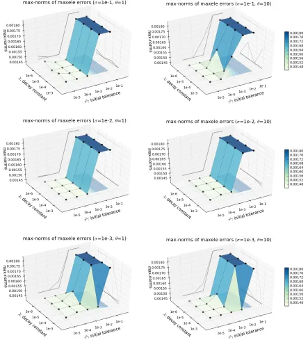
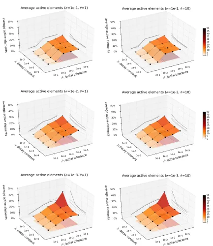
For the parametric study, 144 child domains are concurrently simulated using all combi-nations of the following control parameter settings: τ0 = {10−1,10−2,10−3,10−4,10−5,10−6}, σ={10−1,10−2,10−3},λ={5×10−3,5×10−4,5×10−5,5×10−6},θ={10,100}. Once again, to evaluate the influence of those settings, we perform a baseline run of the parent domain after the same local change has been made to it, and compute the l2-norms and max-norms
of maximum elevation errors of child domains, as shown in Figs. 2.27 and 2.28. The average percentage of active elements for each child domain is shown in Fig. 2.29.
Changes in initial tolerance and the decay constant have the most significant influences while the influences of changes in activation interval and the contraction factor are less significant. As the initial tolerance is reduced, the child domain patches expand further and accuracy improves. Similarly, as the decay constant is increased, the local tolerances converge to the initial tolerance more quickly, and so once again the accuracy improves. The maximum error in maximum elevations is 0.69 cm for the best combination of settings (τ0 = 10−6, σ = 10−3,
(a) (b)
(c) (d)
Figure 2.26: Case 3: Progression of a Walden Creek child domain patch for τ0 = 10−5, σ = 10−2, λ = 5×10⁻⁴, and θ = 10, with elements in the patch darkened. Snapshots: (a) initial extent, (b) extent at timestep 546 520, (c) largest extent (occurring at timestep 570 694), and (d) final extent (timestep 668 367).
Case 4: Brunswick intake canal and Hurricane Irene (2011)
For the final case, we again apply HSM in the context of a hurricane storm surge scenario, but this time using a more refined grid of the western North Atlantic: NC Mesh Version 9.98 with 622 946 nodes and 1 230 430 elements. Otherwise the extent and model parameters mostly correspond to those given in Case 3. For Hurricane Irene, a best-track file from the NOAA NHC online data archive is used for the meteorological forcing, and a 0.5-s step size is used to perform an 8-day simulation of the event as a 2DDI analysis. For this example, no tidal forcing is applied, thereby eliminating a long tidal spin-up run.
the associated Manning’s n values from 0.02 to 0.012, as shown in Fig. 3.10.
Figure 2.30: Case 4: Local change at Brunswick intake canal in the refined Cape Fear subdo-main.
The expansion and contraction of the child domain with ASM control parametersτ0 = 10−3, σ = 10−1,λ = 10−5, and θ = 100 is shown in Fig. 3.11. The patch expands as the hurricane
storm surge approaches, and it reaches its largest extent at timestep 1 203 758 (about 87% of simulated time). As the effects of the hurricane and the altered hydrodynamics dissipate, the patch contracts almost to its original extent.
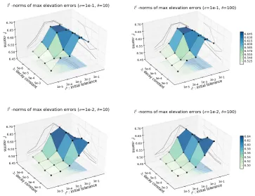
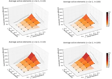
For the parametric study, 96 child domains are concurrently simulated using all com-binations of the following control parameter settings: τ0 = {10−1,10−2,10−3,10−4}, σ =
{10−1,10−2,10−3}, λ = {1×10−5,3×10−6,1×10−6,3×10−7}, θ = {10,100}. As in other cases, we perform a baseline run of the parent domain after the same local change has been made to it, and compute the l2-norms and max-norms of maximum elevation errors of child
domains, as shown in Figs. 2.32 and 2.33. The average percentage of active elements for each child domain is shown in Fig. 2.34.
(a) (b)
(c) (d)
Figure 2.31: Case 4: Progression of a Brunswick child domain patch for τ0 = 10−3,σ = 10−1, λ = 10−5, and θ = 100, with elements in the patch darkened. Snapshots: (a) initial extent, (b) extent at timestep 1 098 072, (c) largest extent (occurring at timestep 1 203 758), (d) final extent (timestep 1 374 294).
τ0 = 10−4, σ = 10−2, λ = 10−6, and θ = 10, and a child domain with τ0 = 10−4, σ = 10−2,
λ= 3×10⁻⁷, and θ = 10. The largest errors of these two child domains, 4.7 cm and 2.2 cm, respectively, are observed to be occurring in wetting and drying regions. Given the nonlinear and discontinuous nature of the wetting and drying algorithm, such discrepancies are sometimes observed to occur, but in very isolated circumstances.
Discussion
In addition to parameter settings, some modeling scenarios are inherently either more or less likely to produce early termination as a result of patches reaching a boundary. For instance, storm surge simulations focusing on overland flows and local changes intopography are usually more robust even for very low initial tolerances, as seen in the Walden Creek example with Hurricane Fran. In other cases, such as the Brunswick intake canal problem, local changes in
bathymetry do influence the hydrodynamics early in the simulation, but less stringent tolerances still allow patches to expand and accommodate those influences appropriately, long before any surge effects come into play. As a result, the ASM technique can accurately simulate diverse modeling conditions, even when local changes occur near grid boundaries, as demonstrated here.
Based on these and other studies we have performed on the accuracy and efficiency of the method, a good balance seems to be found with ASM control parameter values of τ0 = 10−3, σ= 10−1,λ= 10−4, and θ= 10, so these constitute our default settings for ADCIRC++.
2.5.2 Applications and Performance
To further demonstrate subdomain modeling and its computational advantages, we look at the following additional cases:
5. Brunswick intake canal at Southport, NC
Hurricane Irene (2011) simulated as before on the more refined Cape Fear subdomain, but this time over a range of depths and Manning’s n values along the intake canal
6. Silver Lake at Wilmington, NC
Hurricane Fran (1996) simulated on a small portion of the Cape Fear River, with varying values of Manning’s n and depth on a part of the river bank
parents, they also demonstrate the complementary benefits of subdomain modeling approaches realized by HSM.
Case 5: Brunswick intake canal and Hurricane Irene (2011)
Instead of control parameters, in this case we vary bottom surface conditions for a new set of child domains located at the same intake canal of the Brunswick nuclear power plant. Through-out its length, we use a constant Manning’s n value of either 0.012, 0.024, 0.048, or 0.096, which ranges from constructed channel conditions to ones that are unmaintained and have dense brush and weeds. Simultaneously, 17 different changes in depth, from −2 m to 2 m, are made to the original bathymetry of the canal in the parent domain. With recording stations shown in Fig. 2.35, a simulation of the resulting 68 child domains is performed using the following ASM control parameter settings:τ0 = 10−4,σ = 10−2,λ= 10−5, and θ= 100.
Figure 2.35: Case 5: Recording stations at the intake canal.
Fig. 2.36 shows the water surface elevations at each recording station for each of the child domains. Changes in Manning’s n values have little effect except when canal depths are reduced to a point where wetting at the southwest end of the channel is prevented.
Case 6: Silver Lake and Hurricane Fran (1996)
(a) Station 1 (b) Station 2
(c) Station 3 (d) Station 4
Figure 2.36: Case 5: Water surface elevations at intake canal recording stations for varying depths and Manning’s n values.
and 22 223 elements on the Cape Fear River near Silver Lake in Wilmington, NC, as shown in Fig. 2.37.
As a hypothetical problem context, a development activity adjacent to the river seeks mate-rials ecologically best suited to lowering water velocities during a hurricane event. To simulate a range of such materials, Manning’s n values are varied along two rows of nodes (50 nodes in total) in the region shown in the figure. The following Manning’s n values are considered: 0.015, 0.041, 0.067, 0.093, 0.119, 0.145, 0.172, 0.198, 0.224, and 0.250. Additionally, to simulate the effects of planned gabion walls of different sizes, the inner row of nodes closer to the river is adjusted in height ranging from 0 m to 0.5 m increases. With recording stations shown in Fig. 2.38, a simulation of the resulting 60 child domains is performed using the following ASM control parameter settings:τ0 = 10−4,σ = 10−1,λ= 10−4, and θ= 100.
Figure 2.37: Case 6: Local changes on the Cape Fear River.
Figure 2.38: Case 6: Recording stations along the river bank.
by the plots, both roughness and raises in topography can be used, whether separately or in combination, to reduce water velocities during the hurricane event simulated.
Performance
The computational efficiency of ASM depends on numerous factors, including control parameter settings, model settings, and the spatial and temporal extent of the impacts of local changes. We evaluate the performance of the technique for the two cases in this section by comparing runtimes on a 64-core AMD Opteron Processor 6274 workstation using a serial prototype of ADCIRC++, an unoptimized pre-release version that nevertheless comes within about 15% of the (serial) performance of ADCIRC itself.
(a) Station 1 (b) Station 2
(c) Station 3 (d) Station 4
Figure 2.39: Case 6: Velocities at recording stations for varying elevation raises and Man-ning’s n values.
domain runtimes are average values that exclude the computational cost of the parent domains.
Table 2.1: Comparison of computational costs for Case 5.
Runtime CPU hours % of full scale
Full-scale grid 1 488 100
CSM subdomain 102 6.88
ASM child domain 3.62 0.24
Table 2.2: Comparison of computational costs for Case 6.
Runtime CPU hours % of full scale
Full-scale grid 897 100
CSM subdomain 9.32 1.04
ASM child domain 0.19 0.021
for adaptivity since memory management is optimized and changes are infrequent (typically less than once every thousand timesteps on average). As a result, costs for ASM subdomains are largely proportional to their extent.
2.6
Conclusions and future work
Subdomain modeling techniques, whether adaptive or conventional, are designed to assess the effects of incremental changes at an incremental computational cost. Motivated by engineering design and failure scenarios, such techniques also support scientific studies where one or more local properties of a physical domain are varied over a meaningful range of values. Subdomain modeling is predicated on the observation that many changes of interest induce responses with a local extent and without producing effects far from their origins—at least at the space and time scales of interest. Thus, we can eliminate calculations that fall outside the sphere of influence of those changes.
conven-tional subdomains as parents and do so hierarchically to any degree of nesting desired, giving rise to the combined HSM approach we describe.
The dynamic nature of ASM patches and other features, such as inter-domain communica-tion, call for a software architecture that can