COMBINATION OF WAVE SOLUTIONS IN SSI AND STRUCTURAL
NONLINEARITIES
Alexander Tyapin1
1Senior Researcher, BKP-2, Atomenergoproject, Moscow, Russia ([email protected])
ABSTRACT
Current SSI approaches provide a choice between wave solutions available in the frequency domain for linear systems (e.g., in SASSI code) and general (potentially non-linear) solutions available in the time domain. In nuclear industry they used to choose for SSI the first variant, because wave behavior of soil was obviously important, and non-linear behavior of structures was not allowed for the main NPP structures for a long time. However, the last trend in the industry is to consider extreme beyond-design loads, so non-linear analysis of structures becomes a must for designers. Anyhow, wave behavior of soil remains of great importance. So, the current goal in the SSI field is to create a “new generation” tool combining non-linear modeling of a structure (and probably of some finite soil volume near the base mat) with linear modeling of infinite layered inertial soil beyond this finite volume.
The author proposes a new approach to convert the frequency-domain impedances (obtained by SASSI) to the time domain. A certain “road map” of problems to be solved is discussed. Several first steps of this “road map” are already completed; next ones are in process.
INTRODUCTION
Current SSI approaches provide a choice between wave solutions available in the frequency domain for linear systems like in SASSI code, see Lysmer et al, (1980) and general (potentially non-linear) solutions available in the time domain. In nuclear industry they used to choose for SSI the first variant, because wave behavior of soil is obviously important, and non-linear behavior of structures was not allowed for the main NPP structures for a long time. SASSI code with several further reincarnations is an industry standard in SSI analysis providing linear wave solutions in the frequency domain.
However, the last trend in the industry is to consider extreme beyond-design loads, so non-linear analysis of structures becomes a must for designers. Anyhow, wave behavior of soil remains of great importance. So, the current goal in the SSI field is to create a tool for non-linear modeling of a structure (and probably of some finite soil volume near the base mat) along with linear modeling of infinite layered inertial soil beyond this finite volume.
Currently wide range of the true non-linear effects is to be introduced into SSI models and combined with wave effects. This is a real challenge for a “new generation”. Non-linear effects in finite volumes can be numerically studied by a great variety of models available nowadays. Hence, the key issue in SSI model is a special boundary, so the emphasis will be put on it in the further discussion.
GENERAL APPROACH
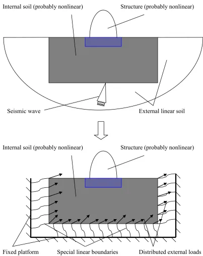
First of all, the next generation SSI models must keep the main available features of the current SSI models. The most important of them is 3D model of SSI. Another one is stratification of soils (today it is horizontal; the author considers it to be enough for the next generation also). The third one is the arbitrary shape of the underground part of structure which is of special importance for Nuclear Power Plants. By the way, this feature enables the consideration of limited soil volume (“near field”) around the basement with special properties (breaking the general stratification) – such soil volume is simply added to the “structural” part of the model, forming the extended underground part.
The first principal new feature of the next generation SSI model must be the applicability of the time-domain analysis necessary to account for the true non-linearity. On the other hand, wave effects in the infinite soil foundation are currently treated as linear ones. In 3D formulation it is unlikely that wave problems for infinite media can be solved in the non-linear approach in the nearest future. So, the conclusion is that the next generation SSI model will consist of two parts: geometrically infinite linear part of the soil foundation (let us call it “far field”) and geometrically finite non-linear part. This second part of SSI model may include a certain “near field” soil and always includes structure. Non-linearity in this finite part may be of different types: material non-linearity (both in “near field” soil and in structure), contact soil-structure non-linearity (loss of soil-structure contact or sliding at the bottom and along the vertical embedded walls), geometrical non-linearity (large displacements), etc.
The tool to model the non-linear “internal” geometrically finite part is obvious: at the moment finite element method (FEM) is simply the best. Real challenge is to combine the internal non-linear part (“near field”) and external linear part (“far field”). As FEM is used for the internal part, there is a certain set of the “interface” nodes, forming the boundary between the internal and the external parts. As the external soil is linear, the forces acting from the external part of soil foundation to these nodes are the sum of two parts. The first part is the “external load” impacting the interface nodes in case they are fixed; this part of the load appears due to the seismic wave (falling and reflected). The second part is the “response load” impacting the interface nodes from the external part of foundation in response to the motion of these nodes (without any seismic waves). The second part of the load is described by the linear operators’ matrix in the time domain; in the frequency domain this matrix turns into the complex frequency– dependent dynamic stiffness matrix. This matrix generally is fully populated. As a result, the SSI model can be schematically presented as shown on Fig.1. This superposition is discussed in Tyapin (2012).
“External loads” and dynamic stiffness represent the infinite linear “far field” in full. In the frequency domain both external loads and nodal dynamic stiffness matrix can be currently obtained by SASSI. External loads can be transferred into the time domain using Fast Fourier Transform (FFT). The remaining part – special boundary in the time domain representing dynamic stiffness matrix – is a key to the whole approach. Classification of different boundaries was given in Wolf (1985). The most popular boundary in the time domain at the moment is that suggested by Lysmer and Kuhlemeyer (1969) several decades ago. It is local (the response force in the node depends on the motion in this node only) and is rigorous only for the body waves normal to the boundary surface. To get reasonable results this boundary should be placed far from the basement.
Figure 1. Scheme of the SSI model. Special boundary (or “soil support”) is described by a fully populated matrix consisting of linear operators (in the time domain) or of the frequency-dependent
complex stiffness terms (in the frequency domain).
Dynamic analysis of the next generation SSI model consists of two stages. The first stage is performed in the frequency domain (e.g., by SASSI) and results in “external loads” and “dynamic stiffness matrix” for the interface nodes. The frequency-domain calculations are performed by SASSI code to get complex frequency-dependent impedance matrix (the conventional one of size 6 x 6 for rigid basement, or nodal extended one 3N x 3N for flexible basement).
Fixed platform
Special linear boundaries
Structure (probably nonlinear)
Internal soil (probably nonlinear)
Distributed external loads
Seismic wave
Structure (probably nonlinear)
Internal soil (probably nonlinear)
Then each element in the impedance matrix is approximated in the frequency domain as a sum of several complex functions of frequency corresponding in the time domain to springs and dashpots with time lags (including conventional zero time lag) with “best-fit” real coefficients. First, time lags are chosen based on frequency dependencies of the translational integral impedances (so far, a single time lag is chosen for each direction, thus generally making three non-zero time lags in addition to one zero time lag). These time lags are taken similar for all elements in the impedance matrices. Then the best-fit approach is used to get “optimal” coefficients - a set of real stiffness and damping matrices corresponding to different time lags will be obtained. As “basic functions” for the best fit procedure are similar for all the elements, the whole procedure is fast and simple even for large and fully populated impedance matrices. “External loads” will be transferred to the time domain using FFT.
After that the second stage will be performed in the time domain by general FEM code. Practical application has been developed by the author using ABAQUS (2008) with user’s subroutines. At every given current time step in the time-domain integration scheme only “zero lag” (i.e. conventional) springs and dashpots contribute to the effective stiffness. All other springs and dashpots (with non-zero time lags) contribute only to the loading forces, as they provide a response to the displacements and velocities, which occurred in the past. The result of the second stage will be the dynamic response of the entire internal part of the SSI model.
“ROAD MAP” AND PRESENT STATUS
To implement the proposed SSI model one has to demonstrate fine solutions of several problems. The author has prepared a draft of the “road map” listing the sequence of such problems. Let us first list the steps and then discuss the present status, as of the beginning of March 2013.
1) Substitution of the dynamic stiffness matrix by a set of real stiffness and damping matrices for several time lags. Procedures to obtain the time lag values and corresponding matrices should be developed. Linear problems are to be solved to compare the time-domain solutions with frequency-domain solutions. These linear problems should include simple structural models listed below starting from the simplest ones:
1.1) rigid surface basements; 1.2) flexible surface basements; 1.3) embedded rigid basements;
1.4) embedded flexible basements and/or near-field soil.
2) Combination of linear “far field” with non-linear “internal part” for surface basements. Different types of nonlinearity should be considered, e.g.
2.1) contact non-linearity (e.g., uplift and sliding);
2.2) structural non-linearity (e.g., elasto-plastic structural elements).
3) The same with embedded “internal part”. Here soil non-linearity (e.g., elasto-plastic soil models) should be used for the “near field”.
Benchmark solutions should be carefully chosen, especially for non-linear calculations. Now let us discuss the present status of these steps.
1) General linear part is already developed. Current version includes a) special procedure to choose time lags and b) standard best-fit procedure to get real matrices of stiffness and damping for these time lags (including zero time lags corresponding to the conventional instant response). There are some ideas how to improve both these procedures.
leading to three real stiffness matrices and three real damping matrices. Time lag values were taken from translational horizontal and vertical impedances. Example is described in details in Tyapin (2013).
1.2) The same structure as in previous sample was analyzed with a flexible base mat. The FE mesh was 8 x 8 - the simplest one allowed by the codes (see ASCE4-98) leading to 9 x 9 =81 nodes over the base mat. Given 3 DOFs a node, that led to fully populated complex frequency-dependent matrix 243 x 243 of nodal impedances. The same procedure as before with the same time lags was applied to the extended matrix, and six real matrices 243 x 243 were obtained. The time-domain solution from ABAQUS was compared to the frequency-domain solution from SASSI in terms of internal bending moments in the mat - this is the most sensible part of the response, see Tyapin (2011). The results proved to be fine; see Tyapin (2013).
1.3) Postponed for a while. 1.4) Postponed for a while.
2) Combination of wave effects and non-linearity is currently on the way.
2.1) Rigid basement is currently analyzed (the same structure, soil matrices and seismic loads as in 1.1). Simplified model of soil-structure contact is used - four corner contact pairs. Uplift without sliding is already done with reasonable results (unfortunately, no benchmark solutions available). Uplift together with sliding is in progress.
2.2) Structural non-linearity will be studied in the future.
3) Embedded internal part of the SSI model will be also studied in the future.
BASIC CONSIDERATIONS
To understand the physical meaning of the time lag stiffness and damping, let us start from 1D linear operator C of the dynamic stiffness. More or less general form of it may be given by Duhamel’s integral
0 00
(
)
(
)
[
(
)
(
)
(
)
(
)]
)]
(
[
x
t
A
x
t
B
x
t
A
x
t
B
x
t
d
C
(1)In the right-hand part of Equation 1 A0 is an “instant” stiffness and B0 is an “instant” damping parameter (two real coefficients). Parameter τ under the integral means time lag, and corresponding stiffness and damping are “distributed over time lag”. This integral may be approximated by a sum, and we get
ni i i i i
t x B t x A t x B t x A t x C 1 0
0 ( ) ( ) [ ( ) ( )]
)] (
[
(2)Number n and values of time lags τi in Equation 2 can be tuned. It is sometimes convenient to treat “instant” coefficients A0 and B0 as the ones corresponding to the “zero time lag”.
After this set of time lags is fixed, stiffness and damping coefficients can be tuned to fit the “target” impedance C(ω) in the frequency domain, known from the other sources prior to the analysis. This step can be done by well-known best-fit technique in the frequency domain. Basic equation here is the Fourier image of the time-lag function and its’ first derivative over time in the frequency domain
U
i
t
d
t
u( ) ( )exp[ ( )]
U i t d i
[exp( ) ( )]exp( ) (3)
i i U i t dt
Let us consider a single non-zero time lag τ spring and dashpot in addition to the conventional “instant” ones. Response force is
)
(
)
(
)
(
)
(
)
(
0
0
1
1
F
t
A
u
t
B
u
t
A
u
t
B
u
t
(5)The Fourier representation of the same force via impedance D(ω) will be
U i t dD t
F
( ) ( ) ( )exp( ) (6)
Using Equation 3 and Equation 4 we come to
1 1
0
0
exp(
)
exp(
)
)
(
A
i
B
i
A
i
i
B
D
(7)It means that non-zero time lag leads to harmonic parts in the frequency-domain impedances, i.e. to local minimums and maximums. Careful study of impedances obtained by SASSI or CLASSI for typical NPP structures in the frequency domain shows that for low frequencies they are rather smooth. In the low frequency interval of usual seismic excitation (up to dozen Hz) there are just one or two local minimums and maximums. This means that several different time lags are enough to get reasonable approximation of impedances. In the next 3D samples the author calculated one non-zero time lag for each translational direction. The value of the time lag was taken from the frequency fmin of the first local minimum of the real part of the impedance ReC(ω) in the corresponding translational direction:
min
2
/
1
f
(8)The example is shown in Tyapin (2013).
The next stage is the best-fit procedure. Equation 7 can be rewritten as
A P
D(
) (
) (9)Here A is a column matrix of real coefficients (A0, B0, A1, B1)T; P(ω) is a line matrix consisting of four elements pj(ω) – complex functions of frequency:
)
exp(
)
(
);
exp(
)
(
;
)
(
;1
)
(
2 3 41
p
i
p
i
p
i
i
p
(10)In fact, Equation 9 means that D(ω) is a linear combination of basic functions pj(ω) with coefficients A.
The goal of the best-fit procedure is to obtain A providing minimum to a functional
D
C
V
d
I
[
(
)
(
)
]
(
)
2
AT{
[(ReP)T(ReP) (ImP)T(ImP)]V 2d
}A
A CV d dV C P C
P)Re( ) Im( )Im( )] 2 } 2
[Re( {
2
(11)
fit to occur. That is why it may be chosen smooth and independent of particular displacement. The author has so far used the empirical formula
0 0
0 )] , 0 2 ; ( ) 0, 2
2 ( [ )
(f f f f f f V f f f
V (12)
Here f0 is a frequency corresponding to the best expected fit between “target” impedance С(ω)
and approximation D(ω) from Equation 9. The author has used f0 = 6 Hz, thus fixing the frequency interval for compliance – it is between zero and 12 Hz.
The further procedure to minimize functional from Equation 11 is standard; it leads to the linear algebraic system with real coefficients
G A
H (13)
Matrix H is as follows (note, that P is a complex line matrix of functions, V is a scalar function of frequency)
d
V
P
P
P
P
H
[(Re
)
T(Re
)
(Im
)
T(Im
)]
2 (14)The right-hand matrix in Equation 13 is as follows
d V C PC P
G [(Re )T Re (Im )T Im ] 2
(15) “Target” impedance values are obtained (e.g., by SASSI) at certain frequencies ωk (k=1,…,m). Linear interpolation is then applied to the impedance in the frequency domain. Interpolation formula for single “target” impedance may be written down asC Q
C(
) (
) (16)Here Q(ω) is a line matrix consisting of m interpolation real functions of frequency qk(ω). Each function qk(ω) is equal to unit in the frequency ωk (k=1,…,m), equal to zero in neighboring frequencies (ωk-1 and ωk+1) and linear between ωk and these neighboring frequencies. Out of the two frequency intervals to the left and to the right of ωk this function is zero. In the right-hand part of Equation 16 C is a vector consisting of m complex values of the impedance C(ω) at frequencies ωk .
Substituting Equation 16 into Equation 15 and using Equation 13 we come to the convenient formulae using real matrices
] Im Re
[ 1 2
1 R C R C
H
A (17)
R P Q V dd V Q P
R T T 2
2 2
1
(Re ) ;
(Im ) (18)These formulae are easily extended for arbitrary number of time lags. Note that H, R1, R2 in Equations 13, 14 do not depend on C; hence, H may be inverted only once. This procedure may be applied to complex frequency-dependent “target” impedance matrices element by element, with the same real matrices H-1R1 and H-1R2 in Equation 17. As a result, we obtain a set of real stiffness and damping matrices for a set of time lags.
and/or embedded flexible basement) the number of boundary nodes will be great. Fully populated matrices will take a lot of space for storage. However, these matrices will stay constant throughout the response analysis. Modern computer codes are able to treat great matrices and the further progress is on the way. Note that the procedure described above is convenient for the parallel computations, because coefficients A in Equation 17 may be obtained element by element in parallel.
After the time lags are fixed and corresponding real stiffness/damping matrices are obtained the time domain calculations follow. Here we see the principal difference between zero and non-zero time lags (we presume that non-zero time lags are greater than time step of integration). “Instant” (i.e. with zero time lags) conventional stiffness and damping contribute to the integration operator; in other words, they contribute to the “left-hand part” of the dynamic equation. One can call them “true” stiffness and damping. On the contrary, stiffness and damping with non-zero time lags contribute to the right part of the same equation, i.e. to the loads. Corresponding “postponed” forces are products of the coefficients and displacements/velocities from the previous time steps. In each particular current time step these forces are already fixed and do not depend on the unknown current displacements/velocities, unlike forces corresponding to the “instant” stiffness and damping. Surely, we do not these “postponed” loads prior to the analysis – we know only “external” seismic loads, impacting the fixed boundary. However, we are able to know total (both “external” and “postponed”) loads at the beginning of each time step, because we already know all the previous displacements and velocities and can estimate their contribution to the current loads.
The author has used ABAQUS so far for the time-domain analysis. User subroutines were written to implement the algorithm described above. Perhaps, this is not the most effective way, but at the first stage of research the results are more important than cost effectiveness.
SAMPLE CALCULATIONS
Linear samples with surface basements (both rigid and flexible) were analyzed successfully; see Tyapin (2011) and Tyapin (2013). Now let us look at sample listed above as 2.1) in the “road map”. Test structure was the same as in Tyapin (2011): a one-store rectangular building 30.6*30.6 m in plan, resting on the surface of the soil foundation. Base mat was 2 m thick; roof was 3 m thick; middle horizontal planes of the base mat and the roof were 7 m one from another. Walls were 1 m thick. Two internal walls were added in vertical planes of symmetry, so each of the four rooms is 15.3*15.3 m in plan.
The whole mass of the building 25570 tones was uniformly distributed over the roof: walls and base mat were assumed weightless.
The roof was assumed rigid; the walls were assumed flexible with real concrete elasticity module
E0=0.3*108 kN/m2. Base mat was assumed flexible; elasticity module was taken variable: E=E
0/fl, where
fl was a flexibility coefficient. This coefficient was varied in the range from zero (rigid base mat) to 1.0 (actual concrete base mat). The internal material damping in the structure was taken 4%. In the time domain Rayleigh damping was used for structure.
Soil foundation was formed by a layer 26 m thick resting on a homogeneous half-space with different wave velocities and damping. Density of the soil was ρ=2.0 t/m3. In the layer shear wave
velocity was Vs=400 m/s; primary wave velocity was Vp=1100 m/s; material damping was 5%. In the homogeneous half-space shear wave velocity was Vs=800 m/s; primary wave velocity was Vp=2100 m/s; damping was 2%.
Single variant of three-component seismic excitation time history was considered. Vertical component had maximal acceleration 0.21g; both horizontal components had maximal acceleration 0.4g.
Figure 2. Scheme of the SSI model for simplified uplift study.
The upper node of the soil support is linked to four corner nodes by rigid weightless beams. Another set of four nodes is linked to the above mentioned corner nodes by very stiff springs. These “another set” nodes are the lower nodes of contact pairs. The upper nodes of contact pairs are actual four corner nodes of base mat. Each contact pair is loaded with compressive static load, equal to the contact force in the static solution (i.e. modeling weight). Seismic excitation in the form of six-component load is applied to the upper node of soil support.
In each contact pair relative horizontal displacements are so far prohibited (on the first stage of research), but relative vertical displacement occurs when tension vertical force in stiff contact spring becomes equal to initial static contact compressive load. That means start of uplift – the gap is open. Tension force then stays equal to static contact load until the gap is closed.
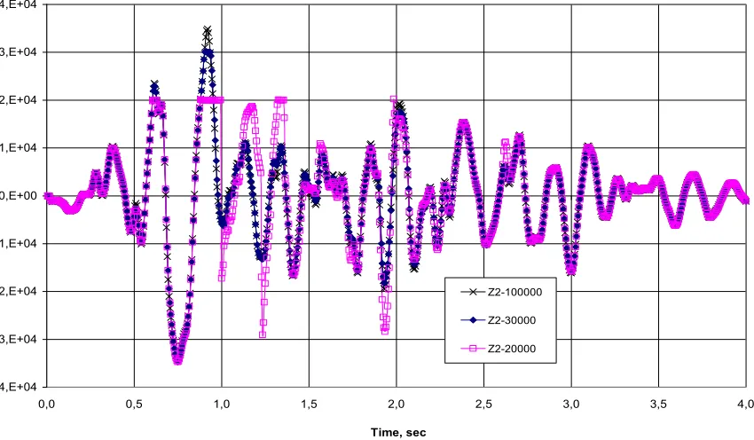
-4,E+04 -3,E+04 -2,E+04 -1,E+04 0,E+00 1,E+04 2,E+04 3,E+04 4,E+04
0,0 0,5 1,0 1,5 2,0 2,5 3,0 3,5 4,0
Time, sec
Z2-100000
Z2-30000
Z2-20000
Figure 3. Time history of vertical forces in one of the corner springs. Compressive contact loads are shown in the legend.
Static contact loads
Upper structure
Contact pairs of nodes
Dynamic seismic load
Stiff springs
In order to reach uplift one can decrease initial static contact loads with the same seismic load instead of increasing seismic excitation. Fig 3 shows time history of the tension force in one of the four corner springs with three different initial contact static loads.
The greatest load (100000 kN) prevents any uplift, and the solution stays linear. The second great contact load (30000 kN) allows only a very short uplift (near the time point 0.9 sec). The lowest contact load (20000 kN) allows considerable uplift, causing sharp peaks of compressive force associated with closure of each gap. For two lower levels of contact load we see that the force in the spring is cut by the contact load, forming the interval of uplift.
This was the first example of combined consideration of the wave effects in infinite linear soil and non-linear effects in “structure”, corresponding to p. 2.1) of the “road map” discussed above. The model is simplified (contact in the corners only; no sliding; rigid plate under the basement), but it demonstrates the principal possibility of such combination. At the moment the author is trying to add sliding to uplift, using Coulomb friction model. Small Coulomb coefficients lead to considerable sliding, eliminating uplift. Greater Coulomb coefficients so far lead to the failure of the computational process in ABAQUS.
CONCLUSIONS
The author proposed a “road map” of problems in order to implement the “new generation” of soil-structure interaction models, accounting both for wave effects in the linear infinite soil media, and for the non-linearity in the structure and in the finite volume of the surrounding soil.
Several starting problems from the presented list have been already solved demonstrating the possibility to transfer wave results obtained in the frequency domain further into the time domain calculations. At the moment the author is implementing non-linearity into the soil-structure interaction model.
REFERENCES
ASCE (1999) Seismic Analysis of Safety-Related Nuclear Structures and Commentary. ASCE4-98.
Reston, Virginia, USA.
ABAQUS (2008). Version 6.8. Dassault Systèmes Simulia Corp., Providence, RI, USA.
Lysmer, J. and Kuhlemeyer, R. (1969) “Finite Dynamic Model for Infinite Media,” J. of Engineering Mechanics Div., ASCE, 95, EM4: 859-877.
Lysmer, J. et al (1981). “SASSI - A Computer System for Dynamic Soil-Structure Interaction Analysis”, Report No. UCB IGT/81-02, University of California, Berkeley.
Tyapin, A. (2010). “Combined Asymptotic Method for Soil-Structure Interaction Analysis // J. Disaster Research. Vol. 5. No.4. 340-350.
Tyapin A. (2011). “The Effects of the Base Mat’s Flexibility on the Structure’s Seismic Response. Part II: Platform Solutions // Proc. SMiRT21. New Delhi. 6-11 November 2011. #266
Tyapin, A. (2012). “Soil-Structure Interaction,” Earthquake Engineering, Halil Sezen (Ed.), ISBN: 978-953-51-0694-4, InTech, Chapter 6. Pp.145-178. Available from:
http://www.intechopen.com/books/earthquake-engineering/soil-structure-interaction.
Tyapin A. (2013). “Next Generation Models for Soil-Structure Interaction Analysis,” J. Disaster Research (to be published).