Same Value Analysis on Edwards
Curves
Rodrigo Abarz´
ua
1, Santi Mart´ınez
2and Valeria Mendoza
1 1Departamento de Matem´
atica y Ciencia de la Computaci´
on,
Universidad de Santiago de Chile, Chile.
1{
rodrigo.abarzua, valeria.mendoza
}
@usach.cl.
2
Departament de Matem`
atica, Universitat de Lleida, Spain.,
2[email protected]
July 21, 2015
Abstract
Recently, several research groups in cryptography have presented new elliptic curve model based on Edwards curves.
These new curves were selected for their good performance and security perspectives.
Cryptosystems based on elliptic curves in embedded devices can be vulnerable to Side-Channel Attacks (SCA), such as the Simple Power Analysis (SPA) or the Differential Power Analysis (DPA).
In this paper, we analyze the existence of special points whose use in SCA is known as Same Value Analysis (SVA), for Edwards curves. These special points show up as internal collisions under power analysis. Our results indicate that no Edwards curve is safe from such an attacks.
Keywords: Elliptic curve cryptography, Side-channel attack, Same value analysis, Edwards curves, Smart cards.
1
Introduction
The demand on wireless technology (cell phones, smart cards, wireless sensor networks etc.) has been increasing in the last years. Most of these devices rely on embedded microprocessors to securely transmit data. Designing efficient cryptographic algorithms is a fundamental problem in the development of secure wireless devices.
Embedded devices present specific problems for implementation of cryp-tosystems. On the one hand, they are computationally limited. On the other hand, they are susceptible to attacks that do not concern conventional cryptog-raphy.
be used without decreasing the security level. For example, some industry standards require 2048 bits for the size of integers1in the RSA system, whereas
the equivalent requirement for elliptic curve cryptography (ECC) is to work with finite fields of 224 bits [20]
In this way, the computations are faster, therefore not so much computing power is needed. Moreover, there is a great interest in the industry to improve the efficiency for the scalar multiplication of points on the elliptic curve, since it is one of the most time consuming operations in ECC protocols [18].
With regard to the second problem, ECC on Smart-Cards can be vulnerable to Passive Side-Channel Attacks. This attack exploit physical leakages from cryptographic process executing on a device, for example: timing [26], power consumption [27] and electromagnetic radiation [19, 34].
There are two general strategies for these attacks: Simple Side-Channel Analysis (SSCA) [26], which analyzes the measurements obtained during a sin-gle scalar multiplication, based on the variations observed in the measurements due to the bit value of the secret key; and Differential Side-channel Analy-sis(DSCA) [27], which is based on statistical techniques to retrieve information about the secret key based on measurements from several scalar multiplications. In 2003 Goubin in [21] presented RPA. The basic idea of this attack is to used special points P0 on the elliptic curve E(K) such that one of the coordinates
is 0 in K. An attacker could construct a point from the elliptic curve used in
the embedded devices, so that depending on the assumed value of a specific bit of the key, she should obtain a special point during the scalar multiplication. An operation which includes a special point is faster and less power consuming than usual. Thus, the attacker can notice when a special point appears and, after several executions, she could obtain the secret key.
Akishita and Takagi in [1] presented a generalization of Goubin’s attacks. An attacker can obtain information not only with the special points, but also when auxiliary registers take the value zero. These new attacks were called Zero Value Point attacks (ZVP-attacks). Akishita and Takagi gave some conditions that, under which, the curve can be attacked through ZVP-attacks.
Murdicaet al. in [32] found another kind of attack in which the attacker can force some points to have collisions, that is to say, they produce some identical values (and identical side-channel traces) during the encryption. This way, she can obtain information about the secret, and after some iterations, she can know the whole secret value. This attack is called Same Value Analysis (SVA).
On the other hand, several groups have presented new elliptic curves for model of Edwards that offer good performance and provide a stronger overall security [3, 5, 8, 9, 22, 28]. Mart´ınezet al. presented an analysis of ZVP points to the Edwards curves, in which they show that these curves are secure against ZVP-attacks [29].
The aim of this paper is to study SVA points for Edwards models. Our results show us that elliptic curves that recently submitted by community, have points that enable SVA-type attacks.
This paper is organized as follows. Section 2 provides an introduction to Edwards curves. Section 3 introduces the SVA points on Edwards and twisted Edwards curves. In Section 4 we presents our experimental results on the exis-tence of SVA points in the new curves Edwards.
Finally, Section 5 concludes the paper.
2
Edwards Curves
Edwards, [17] introduced a new form for elliptic curve:
x2+y2=c2(1 +x2y2),
Every elliptic curve over a non-binary finite field can be birationally trans-formed to an Edwards curve. Some elliptic curves require moving to an exten-sion field for the transformation, but others have transformations defined on the original finite field.
Bernstein and Lange [6] extended the result of Edwards to capture a larger class of elliptic curves over the original field, and introduced their use for cryp-tographic applications. Their model is
E:x2+y2=c2(1 +dx2y2),
where cd(1−c4d)6= 0. The only singular points for these curves is the point
at infinity. The neutral element of the curve is (0, c) and given a pair of points (x1, y1),(x2, y2)∈E the addition law is:
(x1, y1) + (x2, y2) =
x
1y2+y1x2
c(1 +dx1x2y1y2)
, y1y2−x1x2 c(1−dx1x2y1y2)
Whendis not a square, the Edwards addition law is complete: it is defined for all pairs of input points on the Edwards curves. Moreover, this addition law unified, it works for every pair of points, making no distinction between addition, doubling, operations whit the neutral element and symmetries.
Given that inversions in the fields have a high computational cost, Bernstein and Lange [6] also provided a (homogenized) projective coordinates model (X2+
Y2)Z2=c2(Z4+dX2Y2).In which, the point (X1:Y1:Z1), Z16= 0 corresponds
to the affine point (X1/Z1, Y1/Z1). The neutral element is (0 :c : 1) and the
symmetric element of (X1:Y1:Z1) is (−X1:Y1:Z1)
2.1
Addition in projective coordinates
Given two points (X1 :Y1 :Z1) and (X2 :Y2 :Z2) an Edwards elliptic curve,
the addition (X3:Y3:Z3) = (X1:Y1:Z1) + (X2:Y2:Z2) is computed as:
A=Z1Z2, B=A2, C=X1X2, D=Y1Y2,
E=dCD, F =B−E, G=B+E,
X3=AF((X1+Y1)(X2+Y2)−C−D),
Y3=AG(D−C),
2.2
Doubling in projective coordinates
Given a point (X1 : Y1 : Z1) on the Edwards curve, the doubling (X3 : Y3 :
Z3) = 2(X1:Y1:Z1), is computed as:
B = (X1+Y1)2, C=X12, D=Y 2 1,
E=C+D, H= (cZ1)2, J =E−2H,
X3=c(B−E)J,
Y3=cE(C−D),
Z3=EJ.
3
Special Points on Elliptic Curves and
Coun-termeasures
Implementations of ECC may be vulnerable to physical attacks unless spe-cial countermeasures are implemented. These attacks are called Side-Channel Attacks (SCA)[23].
There are several methods to obtain the secret, depending on how many executions are carried out and what kind of information is used. There are three main types of attacks: power, time and electromagnetic attacks (EMA). All attacks can also be divided intoSimple Power Analysis (SPA) andDifferential Power Analysis (DPA).
SPA looks for patterns of computation behavior from the information ob-tained from a single execution. With this information, the attacker tries to guess which operations are being carried out by the embedded devices at every moment, and from this guess the secret used in the cryptosystem. DPA obtains information after several executions. It computes statistical analysis from the information obtained and looks for the most probable key.
In order to obtain the key using timing attacks, the secret must be related to the time needed to process different inputs. In other words, to find variations in the obtained measurements in a given moment in order to obtain the bit that is processed in that moment. If we can obtain the bit at specific steps of the scalar multiplication, after many executions we can obtain the whole secret.
EMA attacks are possible because embedded devices are made of silicon semi-conductors. When the embedded devices is accessed, there is a flow of electrons in the medium, which generates electromagnetic waves. These waves can be captured by an attacker, obtaining information about the operations carried out and giving a chance to guess the secret.
3.1
Refined Power-Analysis (RPA) Attacks
given elliptic curve. The conditions that must avoid an elliptic curve in Weier-strass form should avoid in order that it does not contain any special points are:
bis a quadratic residue inFp . This way, the curve will have (0, y) points.
the elliptic curve has points of order 2, which are (x,0) points.
Smart [37] proposed the use of isogenies in order to avoid RPA, since the fact that a given elliptic curve fulfills the Goubin’s conditions does not mean that its isogenous curves have the same problem.
3.2
Zero-Value Point (ZVP) Attacks
An attacker can also obtain information about the secret if there exists some intermediate parameters, used in the addition or doubling computations, with zero-value. This attack is called Zero-Value Point attack (ZVP-attack).
When an embedded devices is computing, an attacker can know if there is a zero-value involved since the power consumption is lower than usual.
Akishita and Takagi [1, 2] gave conditions for elliptic curves to be vulnerable to this kind of attacks:
ED1. 3x2+a= 0,
ED2. 5x4+ 2ax2−4bx+a2= 0,
ED3. order(P) = 3,
ED4. x(P) = 0 orx(2P) = 0, then bis a quadratic residue,
ED5. y(P) = 0 ory(2P) = 0.
Conditions ED4 and ED5 are those proposed by Goubin.
3.3
Same Value Analysis (SVA) Attacks
Murdicaet al.[32] found another kind of attack in which the attacker can force some points to have collisions, that is to say, they produce some identical values during the encryption. By identifying these values, she can obtain information about the secret, and after some iterations she can know the whole secret value. This attack is called Same Value Analysis (SVA). Murdica, notes that certain special points, internal collisions occur in the operation of doubling Jacobian coordinates, for example, SED conditions come from the doubling of a point P = (x, y):
SED2. x= 0,
SED3. x= 1,
3.4
Recursive attack using special points
Suppose that the attacker already knows the l−i−1 left-most bits of the fixed scalar k= (kl−1, kl−2, . . . , ki+1, ki, ki−1, . . . , k0)2 and wants to recover the
unknown bitki.
The attacker chooses a pointP0satisfying one of the above conditions (SED2
for example), computes the point
P = [(kl−1, kl−2, . . . , ki+1, ki, ki−1, . . . , k0)−21mod #E]P0
and sends thisP to the targeted chip that computes the ECSM using the fixed scalark.Ifki= 0, the pointP0will be doubled during the ECSM, and a collision
of power consumption will appear during the ECSM. The attacker recovers several traces of the power consumption during the computation of [k]P.Using the methodology presented in [35] and [13] to detect internal collision. He can conclude ifki = 0 or not (ki = 1) The attacker can recursively recover all bits
ofk.
3.5
Countermeasures
In this section we present the main countermeasures for RPA, ZVP, and SVA. There are three major families, a) Isogeny, b) Randomizing scalar k and c) Randomizing pointP.
3.5.1 Isogeny Countermeasure
In order to resist RPA for point of large order, Smart [37] proposed to map the underlying curve to the isogenous curve that does not have the point (0, y). To apply the isogeny defense it would be better to alter the standards so that the curves are replaced with isogenous ones. However, since this is unlikely to be an option the smart card needs to convert the input point to the isogenous curve. This countermeasure with a small isogeny degree is faster. However, but it is much slower to implement on a smart card, in [4]. The use of isogenies is more efficient as the same algorithms can be used for point arithmetic with the addition of two transformations. Moreover, these transformations can be defined when a cryptosystem is implemented to minimize the impact on the time taken to compute a scalar multiplication.
Volcanoes Isogeny [31]: Miretet al.[31], presented improvements the com-puting and time to find the suitable isogeny degrees of several SECG standard curves [36]. Miret et al. uses the Isogeny-Volcano. Moreover, evaluated the probability of a curve failing for this condition (ED4: x(P) = 0 or x(2P) = 0, i.e. bis a quadratic residue) is 1/2.
In Table 1 we present the result obtained by Smart in [37] and Miredet al.
in [31]. In the second and fourth column present the minimal and preferred isogeny degree with respect to condition ED4, given by Smart in [37], while the third and the fifth columns contain the degrees of the isogeny-route given by the algorithm presented by Miret in [31]. More precisely, the minimal `std and
preferred isogeny degree`prf can be defined:
`prf : The minimal Isogeny degree for condition ED4 and conditiona=−3.
Table 1: Minimal isogeny degrees with respect to ED4 for SECG curves ED4 `std [37] `std−route [31] `prf[37] `prf-route [31]
P-192 23 5-13 73 5-13-23
P-224 1 1 1 1
P-256 3 3 11 3-5
P-384 19 19 19 19
P-521 5 5 5 5
The integer `std−route and `prf−route correspond to the minimal and
preferred isogeny degree obtained by Miretet al. in [31]. For example, the curve P-192 from NIST the preferred isogeny degree is`prf= 73 while`prf−route=
5−13−23,which means the composition of three isogenies of degrees 5, 13 and 23.
In Table 2 provides the computing and searching time to find the suitable isogeny degrees, as can be seen the volcano-isogeny obtain better calculation and search times, specially when searching for a preferred curve.
Table 2: Time for computing minimal isogeny degrees with respect to ED4 T. Comp./T.Cerca. Methods anterior (seg.) Isogeny-route (seg.)
P-192 (lstd) 44.30/51.24 6.01/ 6.99
P-192 (lprf) 3474.7/4788.15 50.31/59.22
P-256 (lprf) 5.93/6.43 0.035/0.043
To protect against RPA and ZPA attacks, the base point P or the secret scalar kshould be randomized.
3.5.2 Countermeasures Randomization of the Scalar k
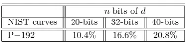
Scalar Randomization [15]: Select a random number d and compute the scalar multiplication Q = [k0]P = [k+d(#E)]P = [k]P+ [d(#E)]P = [k]P, since [d(#E)]P = P∞. Since, the d of size 20-bits. We have considered the
average of percentage of performance loss of curves P−192,
Table 3: Theoretical loss Cost
nbits ofd
NIST curves 20-bits 32-bits 40-bits P−192 10.4% 16.6% 20.8%
Generate a random numberris expensive, this countermeasure requires at least twice the processing both [k−r]P and [r]P need to be computed2.
Trichina-Bellezza Countermeasure [40]: Trichina et al. was proposed the following countermeasure. For any random number r, evaluate [k]P = [kr−1]([r]P).A disadvantage of this countermeasure is required to compute the inverse ofrmodule ordE(P).Besides, two scalar multiplication are needed, first
R= [r]P is computed, then [kr−1]Ris computed.
Euclidean Division [12]: That is, k is written as [k]P = [kmodr]P + [bk/rc]([r]P)
Letting S := [r]P, k1 := kmodr and k2 := bk/rc we can obtain Q =
[k]P = [k1]P+ [k2]Swhere the bit length ofrisn/2.Ciet, presented an regular
algorithm variant of Shamir’s double ladder.
Self-Randomized Exponentiation Algorithms [11]: Letk= (kl, . . . , k0)2=
Pl
i=0ki2i with ki ∈ {0,1} denote the binary representation of exponent k.
Defining
kd→j:= (kd, . . . , kj)2=
X
j≤i≤d
ki2i−j,
The main idea behindself-randomized exponentiationconsists in taking part ofkas a source of randomness. The algorithm relies on the simple observation that, for any 0≤ij ≤l,we have.
[k]P = [kl→0]P
= [kl→0−kl→i1]P+ [kl→i1]P
= [(kl→0−kl→i1)−kl→i2]P+ [kl→i1]P+ [kl→i2]P
=... ... ...
= [(((kl→0−kl→i1)−kl→i2)−kl→i3)· · · −kif]P+ [kl→i1]P
+ [kl→i2]P+ [kl→i3]P+· · ·+ [kl→if]P .
3.5.3 Set of Countermeasures Randomization PointP
Blinding Point [15]: A fixed (secret) point R is selected and S = [k]R is precomputed. GivenP,the computation of [k]Pis replaced by that of [k](P+R) and the known valueS= [k]R is subtracted at the end of the computation.
3.5.4 Countermeasures do not support special points attacks:
Randomized algorithm 2P∗ [12]: Ciet and Joye in [12], proposed the 2∗ Algorithm, this randomization method is applicable to left-to-right scalar multi-plication algorithm. The idea is randomize [2]Pusing the method of randomized projective coordinates. This allows to keep usingP in affine coordinate (which
equivalent to saying that its Z-coordinate of P is equal to 1) and the scalar multiplication is computed in mixed coordinates is used (which is more effi-cient, then using only projective coordinates). Moreover, the algorithm allows using an elliptic curve with parametera=−3.
Randomized field K Isomorphism [24]: The idea of this countermeasure
is to use a representation of random fields definition of elliptic curve, i.e. use a Randomized fieldφ: K→K0 then this isomorphism is used to obtain a point
P0=φ(P) of the curve E0=φ(E), so the scalar multiplication is calculated as
[k]P =φ−1([k](φ(P)))
This countermeasure has the major disadvantage that special fields used in most standards for example NIST and SEGC use irreducible polynomials for which the reduction is much more efficient (for example, in characteristic two using trinomials or pentanomials in which most of the terms have very low degree), this property is usually lost after the field isomorphism is applied, so the operations over the isomorphic fields can be much slower (see [4]).
Randomized E(K) Isomorphism [24] The idea of this countermeasure is
to transfer the base point P1 = (x, y)∈ E1(K) randomly selected isomorphic
curve φ : E1(K) → E2(K) (the parameters of the curve E2(K) are a0 = r4a
and b0 =r6b), the transferred point isφ(P1) = (r2x, r3y) =P2 and the scalar
multiplication is execute as ([k]P2= [k]φ(P1)) on the curveE2(K) and the result
Q2= (xk, yk) is brought back to the original curveE1(K), by computingQ1=
[k]P = (xk/r2, yk/r3) = φ−1([k](φ(P))). The randomization takes 4M + 2S
at the beginning and 1I+ 3M+ 1S at the end. However, when using random curve isomorphisms the parameters ofE2(K) cannot be chosen and one cannot
take advantage of algorithms that require curve parameters to be set to specific values, the curve parameterais randomized. In particular, fast doubling formula fora=−3 cannot be used.
Generalization: Tunstall and Joye, [41]: Define
φ(P) =P0= (X0, Y0, Z0) = (fµX, fνY, Z)
for an arbitraryf ∈ Fp− {0} and some small integerµ and ν.The
in-verse of φ can be computed without inverting f since P = φ−1(P0) = (fνX0, fµY0, fµ+νZ). The caseµ= 2, ν= 3 correspond to the technique of randomizedE(K) isomorphism of Joye and Tymen [24].
Randomized Projective Coordinates [15]: Randomizing the homogeneous projective coordinates of pointP = (X, Y, Z) withλ6= 0 toP = (λX, λY, λZ). The random variable λ can be updated in every execution or after each dou-bling or addition. When we compute the scalar multiplication using Jacobian coordinates, the pointQis represented asQ= (X, Y, Z). The pointQmust be recovered to affine coordinate by computingx=X/Z2andy=Y /Z3and so we
one [38], i.e. scalar multiplication we cannot use mixed coordinates (Jacobian or affine). This countermeasure is effective against Template Attacks [10].
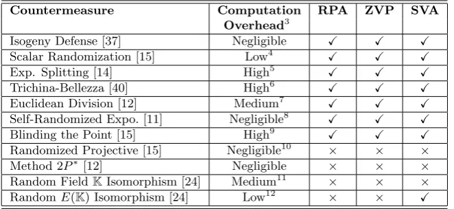
In the following table we present a summary of countermeasures to DPA, each with its overhead cost and whether it is effective (X) or fails (×) against the three types of attacks considered: RPA, ZVP and SVA.
Table 4: Summary Countermeasure
Countermeasure Computation RPA ZVP SVA
Overhead3
Isogeny Defense [37] Negligible X X X
Scalar Randomization [15] Low4
X X X Exp. Splitting [14] High5
X X X Trichina-Bellezza [40] High6
X X X Euclidean Division [12] Medium7
X X X Self-Randomized Expo. [11] Negligible8
X X X Blinding the Point [15] High9
X X X Randomized Projective [15] Negligible10 × × ×
Method 2P∗[12] Negligible × × ×
Random FieldKIsomorphism [24] Medium11 × × × RandomE(K) Isomorphism [24] Low12 × ×
X
In the next session, we present the conditions for the existence of SVA points in the Edwards model, these conditions come from the algorithms for point addition and doubling.
3.6
SVA on Edwards Curves
Given the points P1 = (λ1x1, λ1y1, λ1) andP2 = (λ2x2, λ2y2, λ2), in projective
coordinates on the Edwards curvesE, we now show that the degrees inλ1 and
λ2 of the terms computed during the doubling of P1 or computed during the
addition ofP1and P2 can be used to mount a SVA attacks.
Algorithm 3.6.1 and 3.6.2 give the addition and doubling formulas for Ed-wards curves in projective coordinates. Pairs of terms with matching degrees in λ1 andλ2 are those around which SVA points can be constructed since the
occurrence of a collision between such terms does not depend on the value ofλ1
andλ2.
3High: ≈100%,Medium: (30−70)%,Low: (10−25)%, Negligible: <0.5% 4On average performance loss is 15.9% for the curve P−192.
5To avoid opening the way to new attacks, [k−r]Pand [r]P must be computed separately, doubling the cost of the scalar multiplication (Ebied in[16]).
6Two scalar multiplication are needed.
7Using a regular algorithm variant of Shamir’s double ladder, the algorithm presented by Ciet in [12] cost is n2D+n2A.
8Performance loss is 10Afor a curve to P−192, for details see Alg II in [11].
9This countermeasure is considered inefficient, since it must perform two scalar multipli-cationsS= [k]pand [k](P+R).
10This countermeasure has a very low cost since only a few multiplications are required: 3Mfor the homogeneous representation and 4M+ 1Sfor the Jacobian representation.
Informations on the right show the degrees of the parametersλ1,λ2of each
operand and the result. In the doubling Algorithm, we denote bynan operand with a term λ of degree n. In the addition Algorithm, we denote l1m2 an
operand with a termλ1 of degreel, and a termλ2 of degreem.
3.6.1 Addition
Considering the formulas given in the previous section, we look for conditions so that the points involved in the addition formula can be used to mount an SVA.
Algorithm 1Addition on Edwards Curves
Inputs: P = (λ1x1, λ1y1, λ1) yQ= (λ2x2, λ2y2, λ2)
1: A=Z1·Z2=λ1λ2 (1112←11·12)
2: B=A2=λ2
1λ22 (2122←1112·1112)
3: C=X1·X2=λ1λ2x1x2 (1112←11·12)
4: D=Y1·Y2=λ1λ2y1y2 (1112←11·12)
5: E=dC·D=λ2
1λ22(dx1x2y1y2) (2122←1112·1112)
6: F=B−E=λ2
1λ22(1−dx1x2y1y2) (2122←2122−2122)
7: G=B+E=λ2
1λ22(1 +dx1x2y1y2) (2122←2122+ 2122)
8: H= (X1+Y1)·(X2+Y2)−(C+D)
=λ1λ2[(x1+y1)(x2+y2)−(x1x2+y1y2)] (1112←1112−1112)
9: I=A·F =λ3
1λ32(1−dx1x2y1y2) (3132←1112·2122)
10: X3=I·H =λ41λ 4
2(1−dx1x2y1y2)·
[(x1+y1)(x2+y2)−(x1x2+y1y2)] (4142←3132·1112)
11: J=D−C=λ1λ2(y1y2−x1x2) (1112←1112−1112)
12: K=A·G=λ13λ32(1 +dx1x2y1y2) (3132←1112·2122)
13: Y3=K·J =λ41λ42(1 +dx1x2y1y2)(y1y2−x1x2) (4142←3132·1112)
14: Z3=cF ·G=λ14λ42c[1−(dx1x2y1y2)2] (4142←2122·2122)
In summary we have
Degree ofλ1λ2 Terms
1112: {A, C, D, H, J}
2222: {B, E, F, G}
3132: {I, J}
4142: {X3, Y3, Z3}
x1x2= 1 ⇒A=C, x1y2+y1x2= 1 ⇒A=H,
y1y2= 1 ⇒A=D, x1x2= 0 ⇒D=J,
2x1x2=y1y2 ⇒C=J, (x1+y1)(x2+y2) = 2y1y2 ⇒H =J,
1 =y1y2−x1x2 ⇒A=J, dx1x2y1y2= 1 ⇒B=E,
x1x2=y1y2 ⇒C=D, 2dx1x2y1y2= 0 ⇒I=K,
x1x2=x1y2+y1x2 ⇒C=H, 2dx1x2y1y2= 1 ⇒E=F,
y1y2=x1y2+y1x2 ⇒D=H, x1x2y1y2= 0 ⇒B=F =G,
dx1x2y1y2= 1 ∧ x1y2+y1x2+ 1 +dx1x2y1y2 = 0 ⇒ X3=Z3,
dx1x2y1y2=−1 ∧ y1y2−x1x2−c(1−dx1x2y1y2) = 0 ⇒ Y3=Z.3
3.6.2 Doubling
Similarly, the expressions used also provide for doubling point (X3:Y3:Z3) =
2(X1:Y1:Z1), which are:
Algorithm 2Doubling on Edwards curves
Inputs: P = (X1, Y1, Z1) = (λx1, λy1, λ)
1: B= (X1+Y1)2=λ2(x1+y1)2 (2←1)
2: C=X2
1 =λ2x21 (2←1)
3: D=Y12=λ2y21 (2←1)
4: E=C+D=λ2(x21+y12) (2←2 + 2)
5: H=c(Z12) =cλ2 (2←1)
6: J=E−2H =λ2[(x21+y21)−2c] (2←2−2)
7: K=B−E=λ2[(x1+y1)2−(x21+y21)] (2←2−2)
8: L=C−D=λ2(x12−y21) (2←2−2)
9: X3=cK·J =cλ4[(x21+y1)2−(x21+y12)][(x21+y12)−2c] (4←2·2)
10: Y3=cE·L=cλ4(x41−y41) (4←2·2)
11: Z3=E·J =λ4[(x21+y12)−2c][(x21+y12)−2c] (4←2·2)
In summary we have:
Degree ofλ Terms
2 {B, C, D, E, H, J, K, L}
Conditions where SVA points are presented, for doubling are:
y1= 0 ⇒B =C, B=E, y21=c ⇒D=H,
2x1+y1= 0 ⇒B =C, x21= 2c 2
⇒D=J,
x1= 0 ⇒B =D, B=E, D=E, x21+y21=c2 ⇒E=H,
x1+ 2y1= 0 ⇒B =D, 2c2= 0 ⇒E=J,
(x1+y1)2=c2 ⇒B =H, x21+y 2 1= 3c
2 ⇒H=J,
x1y1+c2= 0 ⇒B =J, x21=c 2
⇒C=H,
x21=y21 ⇒C=D⇒L=Y3, x21+y 2
1= 0 ⇒Y3=Z3,
y12= 2c2 ⇒C=J, y12+c2= 0 ⇒Y3=Z3
x1= 0∧y1= 0 ⇒K=X3= 0.
c(2x1y1(x21+y 2 1−2c
2)−(x4 1−y
4
1)) = 0 ⇒X3=Y3,
(x21+y21−2c2)(2x1y1−x21−y 2
1) = 0 ⇒X3=Z3,
3.6.3 Twisted Edwards Curve
Bernsteinet al. in [7] introduced a generalization of Edwards curves.
LetFq be a non binary field. Then, the twisted Edwards curve with
coeffi-cientsa, d∈Fq satisfyingad(a−d)6= 0, is a curve of the form
EE,a,d:ax2+y2= 1 +dx2y2
Ifa= 1, the previous curve is an Edwards curve, so twisted Edwards curves correspond to a larger set of elliptic curves.
Explicit formula for addition and doubling on twisted Edwards curves are shown in [7]. To avoid inversions, twisted Edwards curves work with projective coordinates where we consider the projective curve
(aX2+Y2)Z2=Z4+dX2Y2,
and (X1:Y1:Z1) withZ16= 0 represents the affine point (XZ11,YZ11).
Addition Give a pair of points (X1 :Y1 :Z1) and (X2: Y2 :Z2), their sum
(X3:Y3:Z3) can be computed as
A=Z1·Z2, B=A2, C=X1·X2, D=Y1·Y2,
E=dC·D, F =B−E, G=B+E,
X3=A·F·((X1+Y1)·(X2+Y2)−C−D),
Y3=A·G·(D−aC),
Z3=F·G .
Algorithm 3Addition on twisted Edwards Curves
Inputs: P = (λ1x1, λ1y1, λ1) yQ= (λ2x2, λ2y2, λ2)
1: A=Z1·Z2=λ1·λ2 (1112←11·12)
2: B=A2=λ21·λ22 (2122←11·12)
3: C=X1·X2=λ1λ2x1x2 (1112←11·12)
4: D=Y1·Y2=λ1λ2y1y2 (1112←11·12)
5: E=dC·D=λ2
1λ22dx1x2y1y2 (2122←11·12)
6: F=B−E=λ2
1λ22[1−dx1x2y1y2] (2122←21−22)
7: G=B+E=λ2
1λ22[1 +dx1x2y1y2] (2122←21+ 22)
8: H=A·F =λ3
1λ32[1−dx1x2y1y2] (3132←1112·2122)
9: I= (X1+Y1)·(X2+Y2)−C−D
=λ1λ2[(x1+y1)(x2+y2)−x1x2−y1y2] (1112←1112)
10: J=A·G=λ3
1λ32(1 +dx1x2y1y2) (3132←1112·2122)
11: K=D−aC=λ1λ2(y1y2−ax1x2) (1112←1112−1112)
12: X3=H·I (4142←3132·1112)
13: Y3=J·K=λ41λ42[1 +dx1x2y1y2][y1y2−ax1x2] (4142←3132·1112)
14: Z3=F·G=λ14λ42[1−(dx1x2y1)2] (4142←2122·2122)
Degree ofλ1λ2 Terms
1112 {A, C, D, I, K}
2122 {B, E, F, G}
3132 {H, J}
4142 {X3, Y3, Z3}
Where internal collisions occur in the following cases:
x1x2= 1 ⇒A=C, dx1x2y1y2= 1 ⇒B=E,
x1x2=y1y2 ⇒C=D, 2dx1x2y1y2= 1 ⇒E=F,
y1y2−ax1x2= 1 ⇒A=K, −ax1x2= 0 ⇒D=K,
x1x2(1 +a) =y1y2 ⇒C=K, x1y2+y1x2= 1 ⇒A=I,
x1x2y1y2= 0 ⇒B=F=G, J=H, x1y2+y1x2=y1y2 ⇒D=I,
x1y2+y1x2=y1y2−ax1x2 ⇒I=K, x1y2+y1x2=x1x2 ⇒C=I,
y1y2= 1 ⇒A=D, Y3=Z3.
Doubling Given a point (X1 :Y1 :Z1), its doubling points is (X3 :Y3 :Z3)
where
B = (X1+Y1)2, C=X12, D=Y12, E=aC,
F =E+D, H=Z2
1 J =F−2H,
X3= (B−C−D)·J,
Y3=F·(E−D),
Algorithm 4Doubling on twisted Edwards curves
Inputs: P = (X1, Y1, Z1) = (λx1, λy1, λ)
1: B= (X1+Y1)2=λ2(x1+y1)2 (2←1)
2: C=X12=λ2x21 (2←1)
3: D=Y2
1 =λ2y21 (2←1)
4: E=aC=aλ2x2
1 (2←2)
5: F=E+D=λ2(y2
1+ax21) (2←2 + 2)
6: H=Z2
1 =λ2 (2←1)
7: 2H = 2λ2 (2←2)
8: J=F−2H=λ2(y2
1+ax21−2) (2←2−2)
9: K=E−D=λ2(ax2
1−y12) (2←2−2)
10: X3= (B−C−D)·J =λ4(2x1y1)(y21+ax21−2) (4←(2−2−2)·2)
11: Y3=F·K=λ4(a2x41−y41) (4←2·2)
12: Z3=F·J =λ4(y12+ax 2 1)(y
2 1+ax
2
1−2) (4←2·2)
In summary we have:
Degree ofλ Terms
2 {B, C, D, E, F, H,2H, J, K}
4 {X3, Y3, Z3}
The internal collisions occur for the following cases:
y1= 0 ⇒B=C, E=F, x1=±1 ⇒C=H
2x1+y1= 0 ⇒B=C, x21−y 2 1 =ax
2
1−2 ⇒C=J
x1= 0 ⇒B=D, B=F, y12=ax21 ⇒D=E
x1+ 2y1= 0 ⇒B=D, ax21= 0 ⇒D=F
(x1+y1)2=ax21 ⇒B=E, y 2
1 = 1 ⇒D=H
x1+ 2y1−ax1= 0 ⇒B=F, ax21−2 = 0 ⇒D=J
x1+y1= 1 ⇒B=H, a= 1 ∧x1=±1 ⇒E =H
x1+y1=−1 ⇒B=H, y12−2 = 0 ⇒E =J
x1=±y1 ⇒C=D y21+ax 2
1= 1 ⇒F =H
a= 1 ⇒C=D, y21+ax21= 3 ⇒H =J
x21=y12 ⇒C=D, 2x1y1=y21+ax 2
1 ⇒X3=Z3
x21=ax21 ⇒C=E, y1=±1 ⇒Y3=Z3
y21+ax21=x21 ⇒C=F,
x1(x1+ 2y1−ax1) = 2⇒B=J,
4
SVA on New Edwards Curves
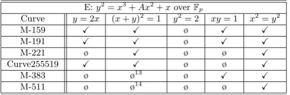
Recently, several research groups have proposed specific curves in Edwards or Twisted Edwards form for use cryptographic application (and possibly future standards) [3, 5, 8, 9, 22]. Our analysis indicates that all these curves have points of SVA type.
In the following table we present the SVA points found
Table 5: SVA Points for Doubling in Edwards curve, birationally equivalent to the Montgomery Curves
E:y2=x3+Ax2+xover
Fp
Curve y= 2x (x+y)2 = 1 y2= 2 xy= 1 x2=y2
M-159 X X ø X X
M-191 X X ø X X
M-221 ø X ø ø X
Curve255519 X X ø ø X
M-383 ø ø13 ø
X X
M-511 ø ø14 ø ø
X
Table 6: SVA Points for Doubling on Edwards Curves
E:x2+y2= 1 +dx2y2 overFp
Curve y= 2x (x+y)2 = 1 y2= 2 xy= 1 x2=y2
E-157 ø X ø X ø
E-168 X ø X ø ø
E-191 ø X ø ø ø
E-222 ø X ø ø ø
Curve1174 ø X ø X ø
E-382 X ø X X ø
Curve41417 X ø ø ø X
E-448-Goldilocks X ø ø ø ø
E-521 ø ø ø X ø
5
Conclusion
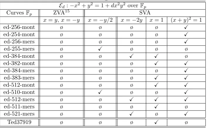
In this paper we analyzed the existence of SVA points in Edwards model of elliptic curves. Our analysis indicates that all curves that have been proposed for cryptographic application are vulnerable to these attacks.
Table 7: SVA Points for Doubling in Twisted Edwards Curves
Ed:−x2+y2= 1 +dx2y2 overFp
CurvesFp ZVA15 SVA
x=y, x=−y x=−y/2 x=−2y x= 1 (x+y)2= 1
ed-256-mont ø ø ø ø X
ed-254-mont ø ø ø ø X
ed-256-mers ø ø ø ø X
ed-255-mers ø X ø ø ø
ed-384-mont ø ø X X ø
ed-382-mont ø ø ø X X
ed-384-mers ø ø ø ø X
ed-383-mers ø ø ø X X
ed-512-mont ø ø ø X X
ed-510-mont ø X ø ø X
ed-512-mers ø ø X X X
ed-511-mers ø ø ø X ø
ed-521-mers ø ø X ø X
Ted37919 ø ø ø X ø
References
[1] T. Akishita and T. Takagi, Zero-Value Point Attacks on Elliptic Curve Cryptosystem, Information Security, ISC 2003, LNCS 2851, pp. 218–233, Springer 2003.
[2] T. Akishita and T. Takagi, On the Optimal Parameter Choice for Elliptic Curve Cryptosystems using Isogeny. PKC 2004, LNCS 2947, pp. 346–359, 2004.
[3] D. Aranha, P. Barreto, G. Pereira and J. Ricardini, A Note on High-Security General-Purpose Elliptic Curves. IARC Cryptology ePrint Archive, Report 2013/647, 2013. http://eprint.iacr.org/
[4] R. Avanzi,Side Channel Attacks on Implementations of Curve-Based Cryp-tographic Primites. Cryptology ePrint Archive Report 2005/017, available from http://eprint.iacr.org/
[5] D. J. Bernstein, Curve25519: New Diffie-Hellman Speed Records. Public Key Cryptography – PKC 2006, volume 3958 of Lecture Notes in Computer Science, pp. 207–228, 2006,
[6] D. J. Bernstein and T. Lange, Faster Addition and Doubling on Elliptic Curves. ASIACRYPT 2007, LNCS 4833, pp. 29–50, Springer 2007.
[7] D. J. Bernstein, P. Birkner, M. Joye, T. Lange, and C. Peters, Twisted Edwards Curves.AFRICACRYPT 2008, LNCS 5023, pp. 389–405, Springer 2008.
Strings. IACR Cryptology ePrint Archive, report 2013/325, 2013. http://eprint.iacr.org/
[9] J. W. Bos, C. Costello, P. Longa, and M. Naehrig,Selecting Elliptic Curves for Cryptography: An Efficiency and Security Analysis. IACR Cryptology ePrint Archive, report 2014/130, 2014. http://eprint.iacr.org/
[10] S. Chari, J. R. Rao, and P. Rohati,Template attacks.Cryptographic Hard-ware and Embedded Systems – CHES 2003 LNCS 2523 pp.13-28 Springer, 2003.
[11] B. Chevallier-Mames. Self-Randomized Exponentiation Algorithms. CT-RSA 2004, LNCS 2964, pp. 236-249, Springer-Verlag 2004.
[12] M. Ciet and M. Joye, (Virtually) Free Randomization Techniques for El-liptic Curve Cryptography.ICICS 2003, LNCS 2836, pp. 348-359, Springer-Verlag 2003
[13] C. Clavier, B. Feix, G. Gagnerot, M. Roussellet, and V. Verneuil,Improved Collision-Correlation Power Analysis on First Order Protected AES.CHES 2011, LNCS 6917, pp. 49–62, Springer 2011.
[14] C. Clavier and M. Joye, Universal Exponentation Algorithm. Crypto-graphic Hardware and Embedded Systems – CHES 2001, LNCS 2162, pp. 300-308, Springer-Verlag, 2001.
[15] J. Coron,Resistance Against Differential Power Analysis for Elliptic Curve Cryptosystems. Cryptographic Hardware and Embedded Systems – CHES 1999, LNCS 1717, pp. 392–302, Springer, 1999.
[16] N. M. Ebeid, Key Randomization Countermeasures to Power Analysis Attacks on Elliptic Curve Cryptosystems. Phd.D. Electrical and Computer Engineering, University of Waterloo.
[17] H. M. Edwards, A Normal Form for Elliptic Curves. Bull. Am. Math. Soc., New Ser.,44(3), pp. 393–422, 2007.
[18] B. Feix and V. Verneuil. There’s Something about m-ary, Fixed-Point Scalar Multiplication Protected against Physical Attacks. INDOCRYPT 2013, LNCS 8250, pp. 197–214, Springer 2013.
[19] K. Gandolfi, C. Mourtel, and F. Olivier, Electronic Analysis: Concrete Results. Cryptographic Hardware and Embedded Systems – CHES 2001, LNCS 2162, pp. 251–261, Springer, 2001.
[20] D. Giry and J.-J. Quinsquater, Bluekrypt Cryptographic Key Length. Rec-ommendation 2011, v26.0, April 18, http://www.keylength.com/.
[21] L. Goubin, A Refined Power-Analysis Attack on Elliptic Curve Cryptosys-tems. Public Key Cryptography, LNCS 2567, pp. 199–210, Springer, 2003.
[22] M. Hamburg, Ed448-Goldilocks, Fast, Strong Elliptic Curve Cryptography.
[23] M. Joye, Elliptic Curves and Side-channel Analysis.ST Journal of System Research, 4(1), pp. 283-306, 2003.
[24] M. Joye and C. Tymen,Protections against Differential Analisis for Elliptic Curve Cryptography. Cryptographic Hardware and Embedded Systems – CHES 2001, LNCS 2162, pp. 377-390. Springer-Verlag, 2001.
[25] N. Koblitz, Elliptic Curve Cryptosystems. Mathematics of Computation,
48, pp. 203–209, 1987.
[26] P. Kocher, Timing Attacks on Implementation of Diffie-Hellman RSA, DSS and other Systems. Advances in Cryptology – CRYPTO 1996, LNCS 1109, pp. 104–113, Springer, 1996.
[27] P. Kocher, J. Jaffe, and B. Jun, Differential power Analisis. Advances in Cryptology –CRYPTO 1999, LNCS 1666, pp. 388–397, Springer, 1999.
[28] P. Longa, Post-Snowden Elliptic Curve Cryptography. Microsoft Research http://research.microsoft.com/en-us/people/plonga/
[29] S. Mart´ınes, D. Sadornil, J. Tena, R. Tom`as, and M. Valls. On Edwards Curves and ZVP-Attacks Applicable Algebra in Engineering Communica-tion and Computing, Vol 24, pp. 507–517, Springer-Verlag 2013.
[30] V. S. Miller, Use of Elliptic Curves in Cryptography. Advances in Cryp-tology – CRYPTO 1985. LNCS 218, pp. 417-426, Springer, 1986.
[31] J. Miret, D. Sadornil, J. Tena, R. Tom`as, and M. Valls. Isogeny Cordillera Algorithm to obtain Cryptographically good Elliptic Curves. Australasian Information Security Workshop: Privacy Enhancing Tecnologies (AISW), CRPIT vol. 68, pp. 127-131, 2007.
[32] C. Murdica, S. Guilley, J-L. Danger, P. Hoogvourst, and D. Naccache,Same Value Power Analysis Using Special Point on Elliptic Curves. COSADE 2012, LNCS 7275, pp. 183-198, Springer-Verlag 2012.
[33] D. Naccache, N. P. Smart, and J. Stern. Projective Coordinates Leak.
EUROCRYPT 2004, LNCS 3027, pp. 257–267. 2004.
[34] J-J. Quisquater, and D. Samyde, Electromagnetic analysis (EMA): Mea-sures and CoutermeaMea-sures for Smard Cards.Smart Card Programming and Security – E-SMART 2001, LNCS 2140, pp. 200–210, Springer, 2001.
[35] K. Schramm, T. Wollinger, and C. Paar, A New Class of Collision At-tacks and Its Application to DES. FSE 2003. LNCS, vol 2887, pp. 206-222 Springer 2003.
[36] STANDARDS FOR EFFICIENTE CRYPTOGRAPHY, SEC 2: Recom-mended Elliptic Curve Domain Parameters. Certicom Corp. Version 2.0, January 2010.
[38] N. P Smart, E. Oswald, and D. Page, Randomised Representations. IET Inf. Secur., 2008, Vol. 2, No 2, pp. 19-27, 2008.
[39] E. G. Strauss. Addition chains of vectors (problem 5125). American Math-ematical Monthly, vol. 70, pp. 806–808, 1964.
[40] E. Trichina and A. Belleza, Implementation of Elliptic Curve Cryptogra-phy with Built-In Counter Measures against Side Channel Attacks. Crypto-graphic Hardware and Embedded Systems, CHES –2002, LNCS 2523, pp. 98–113, Springer 2002.
[41] M. Tunstall and M. Joye, Coordinate Blinding over Large Prime Fields.