HISTORY BASED CONTENTION WINDOW CONTROL PROTOCOL FOR ENERGY EFFICIENCY IN WIRELESS SENSOR NETWORK

HISTORY BASED CONTENTION WINDOW CONTROL

PROTOCOL FOR ENERGY EFFICIENCY IN WIRELESS

SENSOR NETWORK

Abhishek Kaushik

, Parvin Kumar Kaushik

, Sanjay Sharma

Post Graduate Scholar KIET, Ghaziabad,

Asst. Prof, ECE Deptt, KIET, Ghaziabad

3

Prof, ECE Deptt, KIET, Ghaziabad (India)

ABSTRACT

The earlier work described in the literature involves different schemes or algorithm that are implemented at the

network layer or at the physical layer of TCP/IP to endorse energy saving so that the network of any system remains

sustainable for long time. The techniques discussed in this paper uses the history based contention window control

over packet routing in the network layer. The main idea behind this scheme is to control the time of every node

which delivers the packet but if in case the proximity node or network does not accept the incoming packets because

it is busy, then the transmitter node has to either wait or it tries randomly to deliver the same. This causes the whole

system to use more of its energy and this is the main reason that conventionally many other protocols are not good

for the system. But our system and our history based contention window control scheme has proved to be worthy as

it is good in terms of the time allocation providing the system either to wait or to access other node for the

transmission of the system. The energy being consumed has reduced considerably and the efficiency and throughput

has increased because of reduced energy consumption.

Keywords: Ad-Hoc Network, Contention Window, Matlab, Wireless Senor Network

I INTRODUCTION

Wireless Sensor Networks consists of individual nodes that are able to interact with their environment by sensing or

controlling physical parameter; these nodes have to collaborate in order to fulfil their tasks as usually, a single node

is incapable of doing so; and they use wireless communication to enable this collaboration [1].

II WIRELESS SENSOR NETWORK

A sensor network is a deployment of massive numbers of small, inexpensive, self powered devices that can sense,

compute, and communicate with other devices for the purpose of gathering local information to make global

decisions about a physical environment” [1].

Sensor network development was initiated by the United States during the Cold War [2]. A network of acoustic

system of acoustic sensors was called the Sound Surveillance System (SOSUS). Human operators played an

important role in these systems.

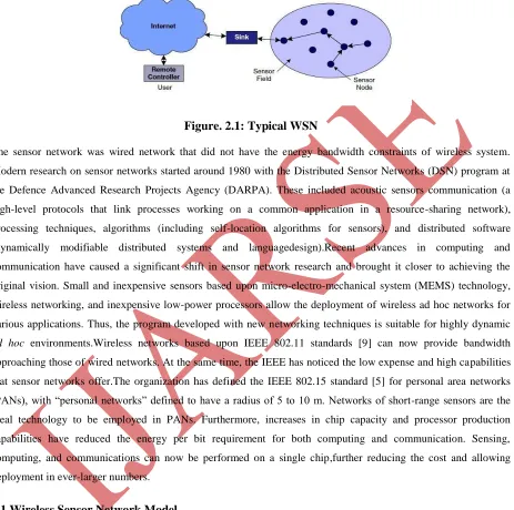
Figure. 2.1: Typical WSN

The sensor network was wired network that did not have the energy bandwidth constraints of wireless system.

Modern research on sensor networks started around 1980 with the Distributed Sensor Networks (DSN) program at

the Defence Advanced Research Projects Agency (DARPA). These included acoustic sensors communication (a

high-level protocols that link processes working on a common application in a resource-sharing network),

processing techniques, algorithms (including self-location algorithms for sensors), and distributed software

(dynamically modifiable distributed systems and languagedesign).Recent advances in computing and

communication have caused a significant shift in sensor network research and brought it closer to achieving the

original vision. Small and inexpensive sensors based upon micro-electro-mechanical system (MEMS) technology,

wireless networking, and inexpensive low-power processors allow the deployment of wireless ad hoc networks for

various applications. Thus, the program developed with new networking techniques is suitable for highly dynamic

ad hoc environments.Wireless networks based upon IEEE 802.11 standards [9] can now provide bandwidth

approaching those of wired networks. At the same time, the IEEE has noticed the low expense and high capabilities

that sensor networks offer.The organization has defined the IEEE 802.15 standard [5] for personal area networks

(PANs), with “personal networks” defined to have a radius of 5 to 10 m. Networks of short-range sensors are the ideal technology to be employed in PANs. Furthermore, increases in chip capacity and processor production

capabilities have reduced the energy per bit requirement for both computing and communication. Sensing,

computing, and communications can now be performed on a single chip,further reducing the cost and allowing

deployment in ever-larger numbers.

2.1 Wireless Sensor Network Model

Unlike their ancestor ad-hoc networks, WSNs are resource limited, they are deployed densely, they are prone to

failures, the number of nodes in WSNs is several orders higher than that of ad hoc networks, WSN network topology

is constantly changing, WSNs use broadcast communication mediums and finally sensor nodes don’t have a global

identification tags [3]. The major components of a typical sensor network are:

 Sensor Nodes: Sensors nodes are the heart of the network. They are in charge ofcollecting data and routing

this information back to a sink.

 Sink: A sink is a sensor node with the specific task of receiving, processing andstoring data from the other

sensor nodes. They serve to reduce the total number ofmessages that need to be sent, hence reducing the

overall energy requirements ofthe network. Sinks are also known as data aggregation points.

 Task Manager: The task manager also known as base station is a centralised point of control within the

network, which extracts information from the network and disseminates control information back into the

network. It also serves as a gateway to other networks, a powerful data processing and storage centre and

an access point for a human interface. The base station is either a laptop or a work station.

Data is streamed to these workstations either via the internet, wireless channels, satellite etc. So, hundreds to several

thousand nodes are deployed throughout a sensor field to create a wireless multi-hop network. Nodes can use

wireless communication media such as infrared, radio, optical media or Bluetooth for their communications. The

transmission range of the nodes varies according to the communication protocol is used.

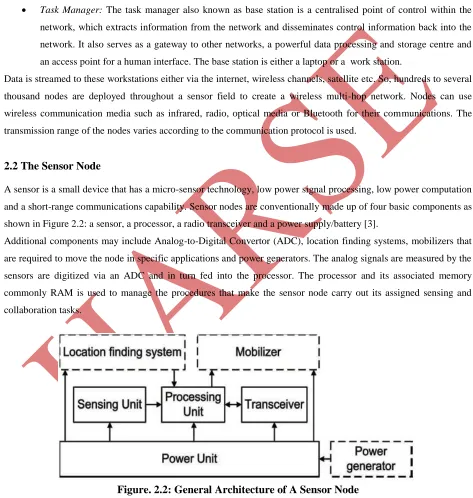
2.2 The Sensor Node

A sensor is a small device that has a micro-sensor technology, low power signal processing, low power computation

and a short-range communications capability. Sensor nodes are conventionally made up of four basic components as

shown in Figure 2.2: a sensor, a processor, a radio transceiver and a power supply/battery [3].

Additional components may include Analog-to-Digital Convertor (ADC), location finding systems, mobilizers that

are required to move the node in specific applications and power generators. The analog signals are measured by the

sensors are digitized via an ADC and in turn fed into the processor. The processor and its associated memory

commonly RAM is used to manage the procedures that make the sensor node carry out its assigned sensing and

collaboration tasks.

Figure. 2.2: General Architecture of A Sensor Node

The radio transceiver connects the node with the network and serves as the communication medium of the node.

Memories like EEPROM or flash are used to store the program code. The power supply/battery is the most

size limitations of AA batteries or quartz, cells are used as the primary sources of power. To give an indication of

the energy consumption involved, the average sensor node will expend approximately 4.8mA receiving a message,

12mA transmits a packet and 5μA sleeping [3]. In addition the CPU uses on average 5.5mA when in active mode.

III PROBLEM IDENTIFICATION & ISSUES

3.1 Cellular and Ad Hoc Wireless Networks

The current cellular networks are classified as the infrastructure dependent networks. The path setup between two

nodes is completed through the base station. Ad hoc wireless networks are capable of operating without the support

of any fixed infrastructure. The absence of any central control system makes the routing complex compared to

cellular networks. The path setup between two nodes in ad hoc network is done through intermediate nodes. For the

distributive system to work the mobile nodes of ad hoc network are needed to be more complex than that of cellular

networks.

3.2 Exposed Teminal problem

In wireless networks, the exposed node problem occurs when a node is prevented from sending packets to other

nodes due to a neighboring transmitter. Consider an example of 4 nodes labeled R1, S1, S2, and R2, where the two

receivers are out of range of each other, yet the two transmitters in the middle are in range of each other. Here, if a

transmission between S1 and R1 is taking place, node S2 is prevented from transmitting to R2 as it concludes after

carrier sense that it will interfere with the transmission by its neighbor S1. However note that R2 could still receive

the transmission of S2 without interference because it is out of range from S1 .

(a)currently transmitting (b) Wish to transmit

Figure 3.1: Exposed Terminal Problem

3.2 Algorithm for RTS Threshold

To set the RTS-Threshold dynamically, we need to observe the current distribution of packet size in the network.

But for this, we need information from all the active nodes. This necessitates inter-layer communication

𝑃

= 𝑃

𝑆 ≤ 𝑠

= (

𝑓

𝑖 𝑗 =1

𝑓

𝑛 𝑘=1

)

Let, Pr is the greatest probability less then η, Ps is the packet size at Pr, Cr is the least probability greater then η, and

Cs is the packet size at Cr. Using linear interpolation the traffic observer calculates the current RTS-Threshold using

the equation below

𝑅𝑇

= 𝑃

+

𝜂 − 𝑃

∗ (𝐶

− 𝑃

)

(𝐶

− 𝑃

)

The average RTS-Threshold is updated as

𝑅𝑇

= 𝛼 ∗ 𝑅𝑇

+ 1 − 𝛼 ∗ 𝑅𝑇

where, RTpreview= previous Threshold and controls the relative weight of recent andpast history of

RTS-Threshold calculation. The value of α lies between 0 to 1.

IV MATERIALS AND METHODS

We propose a novel backoff mechanism, in which the history of packet lost is taken into account for Contention

Window size optimization. The packet lost involves packet collision and channel error.In this study, we utilize two

parameters x and y, that are used to update CW value. We check the channel and if the packet lost rate is increased

because of channel error or collision, we increase the CW size for decreasing the packet lost and when the packet

lost rate of the channel is decreased we decrease the CW size slowly for increasing the throughput. The CS (Channel

State) is three elements array that is updated upon each transmission trial, i.e. each time the station transmits the

packet successfully and receives the acknowledgement (ACK for data and CTS for RTS packets) or when the packet

becomes collide because of channel error or collision. When we store the new channel state, the oldest channel state

in the CS array is removed and the remaining stored states are shifted to the left.

V SIMULATION AND RESULTS

The first section calculates the different network data by using some data nodes transmission time acknowledgement

packets, transmitted packets and many other requirements. The second section discusses the same using a GUI built

in MATLAB R 2010a version which tries to bring upon user and programming interface in a lucid fashion.

 Three types of simulation schemes have been preferred over the entire network.  There is one channel model AWGN used in the simulations.

 The different outputs of the simulation are: estimate of successful, acknowledged and failed packets.

The table 5.1 describes the work of two different authors and there comparison with the work done in the thesis. The

window. The work done by the authors are referenced and their respective results are also discussed. The thesis

strives to give better results by using iterative clipping and filtering techniques, which is a low cost better

performing technique when compared on the cumulative distribution function. In the work proposed History based

contention window tends to give good results, which is required.

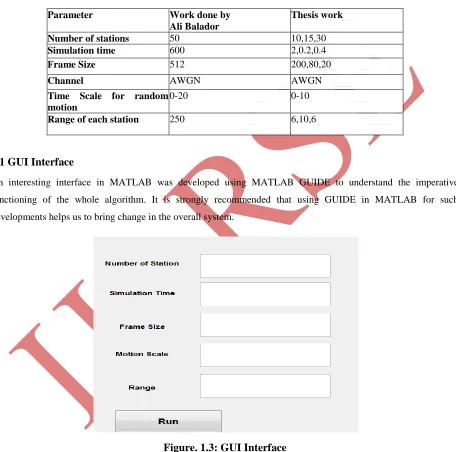
Table 5.1: Simulation Parameters

Parameter Work done by

Ali Balador

Thesis work

Number of stations 50 10,15,30

Simulation time 600 2,0.2,0.4

Frame Size 512 200,80,20

Channel AWGN AWGN

Time Scale for random motion

0-20 0-10

Range of each station 250 6,10,6

5.1 GUI Interface

An interesting interface in MATLAB was developed using MATLAB GUIDE to understand the imperative

functioning of the whole algorithm. It is strongly recommended that using GUIDE in MATLAB for such

developments helps us to bring change in the overall system.

Figure. 1.3: GUI Interface

The report intents to bring upon the subject of energy utilisation using different schemes out of which the thesis

provides a step by step approach towards the development of the entire model over the same subject. The initial step

was to design those pre requisites inputs which are towards the progress of the model. There is small figure which

Next is the section in wholesome which has different outputs produced as the part of the thesis. The overall section

of output is again shown as a figure in the report.

Figure. 1.4: GUI Interface

The final development of the guide includes the different figures clubbed all together to enhance the feature of the

complete system.

Figure. 1.5: Overall GUI Interface

It has tried to give better outputs over the same simulation by using DCF scheme and projecting using HBCWC as

the proposed matter. Later in the section another important task is to consider the final results which the thesis has

tried to showcase. The results are discussed for different users, simulation time and many other parameters given in

the Table No 1.2. The important parameter which has the frame size for the base is 512 packets and 200, 80, 20

VI CONCLUSION

Routing is a significant issue in Wireless Sensor Networks. The objectives listed in the problem statement have been

carried out properly. We sincerely hope that our work will contribute in providing further research directions in the

area of routing. Since energy of the nodes is a constraint in wireless sensor network, so a fix amount of energy is

given to the network. As the simulation time increases, nodes in the network continuously lose its energy and after a

fix simulation time network collapse.

ACKNOWLEDGEMENTS

I would like to express my sincere thanks to my esteemed and worthy supervisor, Mr. ParvinKaushik Assistant

Professor, Department of Electronics and Communication Engineering, KIET Ghaiziabad for his valuable guidance

in carrying out this paper. I would like to express sincere thanks to Dr. Sanjay Sharma,Professor, Department of

Electronics and Communication Engineering,KIET Ghaziabad, for his moral support, effective supervision and

encouragement.

REFERENCES

[1] Akyildiz I., Su W., and Sankarasubramaniam Y., 2002. “A survey on sensor networks”, IEEE Commun. Mag.,

vol. 40, no. 8, pp. 102–114.

[2] Yick J., Mukherjee B., and Ghosa D., 2008. “Wireless sensor network survey”, Computer Networks, vol. 52, no.

12, pp. 2292–2230.

[3] Kuorilehto M., Hannikainen M., and Hamalainen T. D., 2005. “A survey of application distribution in wireless

sensor networks”, EURASIP Journal onWireless Communications and Networking, vol. 2005, no. 5, pp. 774–

778.

[4] Alemdar H. and Ersoy C., 2010. “Wireless sensor networks for healthcare: a survey”, Computer Networks, vol.

54, no. 15, pp. 2688–2710.

[5] Chee-Yee C. and Kumar S. P., 2003. “Sensor networks: evolution, opportunities, and challenges”, Proceedings

of IEEE, vol. 91, no. 8, pp. 1247–1256.

[6] Pantazis N. A. and Vergados D. D., 2007. “A survey on power control issues in wireless sensor networks”,

IEEE Commun. Surveys Tuts., vol. 9, no. 4, pp. 86– 107.

[7] Chang J. H. and Tassiulas L., 2000. “Energy conserving routing in wireless adhoc networks”, Proc. IEEE

International Conference on ComputerCommunications INFOCOM2000, Tel-Aviv, Israel, pp. 22–31.

[8] Mahfoudh S. and Minet P., 2008. “Survey of energy efficient strategies in wireless ad hoc and sensor networks”,

Proc. Seventh International Conference onNetworking ICN 2008, Cancun, Mexico, pp. 1–7.

[9] Bandyopadhyay S. and Coyle E. J., 2003. “An energy efficient hierarchical clustering algorithm for wireless