University of South Carolina
Scholar Commons
Theses and Dissertations
2016
Measurement of New Observables from the π + π
-Electroproduction off the Proton
Arjun Trivedi
University of South Carolina
Follow this and additional works at:https://scholarcommons.sc.edu/etd
Part of thePhysics Commons
This Open Access Dissertation is brought to you by Scholar Commons. It has been accepted for inclusion in Theses and Dissertations by an authorized administrator of Scholar Commons. For more information, please [email protected].
Recommended Citation
Trivedi, A.(2016).Measurement of New Observables from the π + π - Electroproduction off the Proton.(Doctoral dissertation). Retrieved
Measurement of New Observables from the π+π− Electroproduction off the Proton
by
Arjun Trivedi
Bachelor of Science
Florida Institute of Technology 2004
Submitted in Partial Fulfillment of the Requirements
for the Degree of Doctor of Philosophy in
Physics
College of Arts and Sciences
University of South Carolina
2016
Accepted by:
Ralf Gothe, Major Professor
Steffen Strauch, Committee Member
Matthias Schindler, Committee Member
Viktor Mokeev, Committee Member
c
Copyright by Arjun Trivedi, 2016
Abstract
Knowledge of the Universe as constructed by human beings, in order to tackle its
complexity, can be thought to be organized at varying scales at which it is observed.
Implicit in such an approach is the idea of a smooth evolution of knowledge between
scales and, therefore, access to how Nature constructs the visible Universe beginning
from its most fundamental constituents. New and, in a sense, fundamental
phenom-ena may typically be emergent as the scale of observation changes. The study of the
Strong Interaction, which is responsible for the construction of the bulk of the visible
matter in the Universe (98% by mass), in this sense, is a labor of exploring evolutions
and unifying aspects of its knowledge found at varying scales ranging from
interac-tion of quarks and gluons as represented by the theory of Quantum Chromodynamics
(QCD) at small space-time scale to emerging dressed quark and even meson-baryon
degrees of freedom mostly described by effective models as the space-time scale
in-creases. A direct effort to study the Strong Interaction over this scale forms the basis
of an international collaborative effort often referred to as the N* program. The
core work of this thesis is an experimental analysis prompted by the need to measure
experimental observables that are of particular interest to the theory-experiment
epis-temological framework of this collaboration. While the core of this thesis, therefore,
discusses the nature of the experimental analysis and presents its results which will
serve as input to the N* program’s epistemological framework, the particular nature
of this framework in the context of not only the Strong Interaction, but also that of
the physical science and human knowledge in general will be used to motivate and
Table of Contents
Abstract . . . iii
List of Tables . . . vii
List of Figures . . . viii
Chapter 1 Introduction . . . 1
1.1 Motivation . . . 1
1.2 N* program . . . 8
1.3 Observables from the electro-production ofpπ+π− off the proton . . . 9
Chapter 2 Extraction of Observables from Experimental Data 12 2.1 Single-differential observables . . . 14
2.2 Photon polarization dependent cross-sections . . . 15
2.3 Summary . . . 18
Chapter 3 Experiment . . . 19
3.1 The Drift Chambers (DC) . . . 21
3.2 Cherenkov Counters (CC) . . . 22
3.3 Time-of-Flight Counter (SC) . . . 24
3.4 Electromagnetic Calorimeter (EC) . . . 26
3.5 Experimental Data . . . 28
Chapter 4 Core Analysis Details . . . 29
4.3 Constants . . . 30
Chapter 5 Particle Identification . . . 32
5.1 Electron Identification . . . 33
5.2 Hadron Identification . . . 41
Chapter 6 Fiducial Boundary Identification . . . 47
6.1 Electron Fiducial Cuts . . . 48
6.2 Hadron Fiducial Cuts . . . 52
Chapter 7 Detector Inefficiency Identification . . . 54
Chapter 8 Momentum and Energy Loss Corrections . . . 59
Chapter 9 Event Selection . . . 62
Chapter 10 Acceptance Calculation . . . 65
10.1 Model Independent Extraction of Acceptance . . . 66
10.2 Simulation Process . . . 69
10.3 Acceptance . . . 70
Chapter 11 Radiative Effects Correction . . . 73
Chapter 12 Estimating Experimental Yield in the Kinematical Holes . . . 75
Chapter 13 Results . . . 78
13.1 Systematic Uncertainties . . . 78
13.2 Overview of the Q2−W kinematic coverage of the E16 experiment . 80 13.3 Singe-differential cross-sections . . . 80
Bibliography . . . 85
Appendix A Process of filling Holes in experimental data . . . . 88
Appendix B Results: Single Differential Cross-sections . . . 90
Appendix C Results: R2T
Xij
φi +R2L
Xij
φi . . . 127
Appendix D Results: R2LT
c,Xij
φi . . . 164
Appendix E Results: R2T T
c,Xij
φi . . . 201
Appendix F Results: R2LT
s,Xij
φi . . . 238
Appendix G Results: R2T T
s2,Xij
List of Tables
List of Figures
Figure 1.1 Epistemological framework of the N* program [1]. . . 8
Figure 1.2 Illustration of the angular kinematics of variable set 1. Left
side: θπ−, φπ−. Right side: α
[p0π+][pπ−]. . . 11
Figure 3.1 Schematic overview of CEBAF reproduced from [22]. . . 20
Figure 3.2 Schematic overview of CLAS reproduced from [23]. . . 20
Figure 3.3 A portion of the two superlayers within the DC reproduced from [19]. 23
Figure 3.4 Illustration of a CC element and the process of the generation
and subsequent collection of the Cherenkov light by the PMT.
Figure is reproduced from [18]. . . 24
Figure 3.5 Illustration of the overall geometry of the SC within a sector
taken from [20]. . . 25
Figure 3.6 Illustration of the U,V and W layers that comprise the 39
passive-active sandwiched layers of the EC detector within a
sector. The figure is reproduced from [17]. . . 27
Figure 5.1 Illustration of the reconstructedz-vertex postion before (black)
and after (blue)z-vertex corrections, and the standardz-vertex
cut (green) at −8.0cm and −8.0cm. . . 34
Figure 5.2 Illustration of the photoelectron cut all the left PMTs of CC
in sector 1: The blue points represent that data points and
the green dotted line the fit to the parametrized Poisson
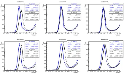
Figure 5.3 Illustration of the SF cut for all sectors: The magenta and
black lines represent cuts obtained by optimizing the fits to fit
at least the peak-bins and maximal-bins of the SF distribution,
respectively, in each momentum bin. . . 40
Figure 5.4 Illustration of the Gaussian fit to SF for momentum bin [1.64GeV, 1.74GeV). . . 41
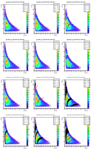
Figure 5.5 Illustration of the ∆t-cut for the protons (top) and positive pions (bottom). . . 44
Figure 5.6 Illustration of the low and high momentum projections of ∆t and their respective fits for the protons. . . 45
Figure 5.7 Illustration of the low and high momentum projections of ∆t and their respective fits for the positive pions. . . 46
Figure 6.1 Illustration of fiducial cuts for electrons of momentum in range [2.20GeV,2.40GeV]. . . 49
Figure 6.2 Illustration of fiducial cuts for electrons of momentum in range [2.50GeV,2.80GeV]. . . 49
Figure 6.3 Illustration of fiducial cuts for electrons of momentum in range [2.80GeV,3.00GeV]. . . 50
Figure 6.4 Illustration of fiducial cuts for electrons of momentum in range [3.00GeV,3.20GeV]. . . 50
Figure 6.5 Illustration of fiducial cuts for electrons of momentum in range [3.40GeV,3.60GeV]. . . 51
Figure 6.6 Illustration of fiducial cuts for protons. . . 52
Figure 6.7 Illustration of fiducial cuts for positive pions. . . 53
Figure 7.1 Cuts to remove inefficient detector regions for the electron. . . 55
Figure 7.3 Cuts to remove inefficient detector regions for the positive pion. . 57
Figure 8.1 Effect of momentum corrections for electrons on the Elastic peak. 61
Figure 8.2 Effect of momentum correction for electron and positive pion,
and energy loss correction for the proton, on the missing mass
distribution for various W bins (integrated over allQ2 bins). . . . 61
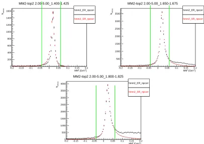
Figure 9.1 M M2 distribution from experimental (black) and simulation
(red) data in W bins from the low, middle and high W range
of the analysis (integrated over allQ2). . . . 63
Figure 9.2 M Mdistribution from experimental (black) and simulation (red)
data in W bins from the low, middle and high W range of the
analysis (integrated over all Q2). . . . . 64
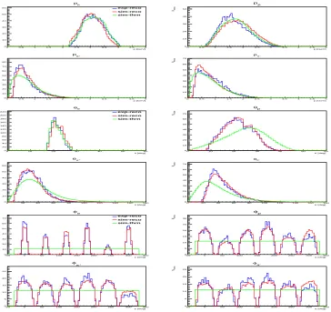
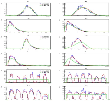
Figure 10.1 Comparison of the final state kinematics forQ2 = [2.0GeV2,3.0GeV2): the blue, red and green lines represent experimental,
simulated-reconstructed and simulated-thrown data, respectively. . . 67
Figure 10.2 Comparison of the final state kinematics forQ2 = [3.0GeV2,5.0GeV2): the blue, red and green lines represent experimental,
simulated-reconstructed and simulated-thrown data, respectively. . . 68
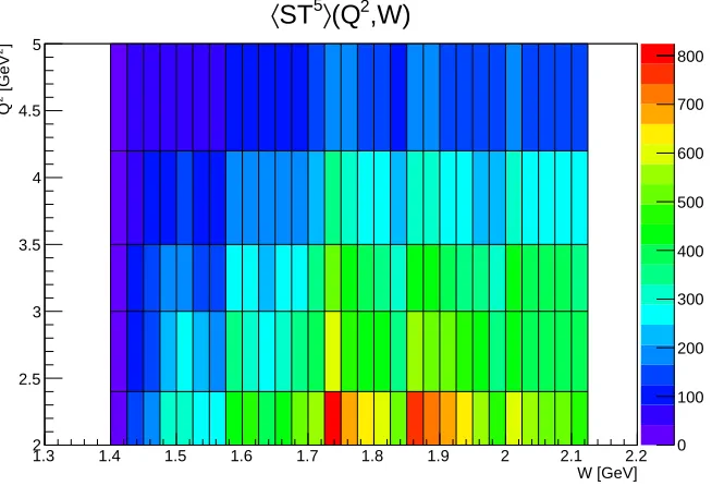
Figure 10.3 Average number of thrown ep → e0p0π+π−events within a 5D
cell within aQ2−W bin, labeled < ST5 >. . . . 71
Figure 10.4 Average number of cut-surviving thrown ep → e0p0π+π−events
within a 5D cell within aQ2−W bin, labeled < SR5 >. . . 72
Figure 10.5 Average 5D acceptance within Q2−W bins, labeled < SA5 >. . . 72
Figure 11.1 Radiative effects correction factor plotted as a function of W
Figure 12.1 Fraction of 5D bins within aQ2−W bin that are identified to
be kinematical holes. . . 76
Figure 12.2 Illustation of the kinematical-hole filling effect: Integrated
cross-sections before and after kinematic-hole filling(top), and the
rel-ative contribution of this process to the measured cross-sections
(below). . . 77
Figure 13.1 Q2−W kinematic coverage of experiment E16. . . 80
Figure 13.2 Single Differential Cross-sections forQ2 = [2.40GeV2,3.00GeV2)
and W = [1.725GeV,1.750GeV). . . 81
Figure 13.3 R2T Xij
φi +R2L
Xij
φi for Q
2 = [2.40 GeV2,3.00 GeV2) and W =
[1.725 GeV,1.750 GeV). . . 82
Figure 13.4 R2LT
c,Xij
φi forQ
2 = [2.40GeV2,3.00GeV2) andW = [1.725GeV,
1.750 GeV). . . 83 Figure 13.5 R2T T
c,Xij
φi forQ
2 = [2.40GeV2,3.00GeV2) andW = [1.725 GeV,
1.750 GeV). . . 83
Figure 13.6 R2LT
s,Xij
φi forQ
2 = [2.40GeV2,3.00GeV2) andW = [1.725 GeV,
1.750 GeV). . . 84 Figure 13.7 R2T T
s2,Xij
φi forQ
2 = [2.40GeV2,3.00GeV2) andW = [1.725 GeV,
Chapter 1
Introduction
1.1 Motivation
Human experience in the observable Universe forms the context upon which human
beings construct knowledge, referred to as human knowledge in this thesis. This
context is arguably and for practical purposes, infinite. This is in the sense that
neither is it possible, thus far, to quantify this context in any analytical language nor
encapsulate a feeling for this context in any qualitative expression.
Just as this context is infinite, so is human knowledge, with its uncountable
quan-titative and qualitative expressions of its understanding of this infinite context.
A perspective that can attempt to contain, and then imagine this infinite human
knowledge based on an infinite context, can be formed by thinking of the experience
of human beings at various points in this context giving rise to domains of human
knowledge centered at each point of experience. Each domain can be thought to have
a finite extent which can be called the sub-context. In this perspective, an infinitely
complex context-space can be thought to contain an infinitely complex configuration
of domains or sub-contexts, within which is contained human knowledge specific to
the domain, which we can call sub-knowledge.
In order to continue motivating this thesis and present its most immediate
mo-tivation, one of the dimensions of this context-space along which several domains
of human knowledge can be more specifically conceptualized will be isolated. This
stretching to infinitely large extents of space-time at one end, and that of
infinites-imally small extents on the other end. The infinitely large extents can be thought
to be the domain of the sub-knowledge fields of Cosmology and Astronomy, and the
infinitesimally small extents that of the fields of Nuclear and Particle physics, and the
range in between can be broadly thought to be the domain of Life, Social, and Earth
sciences in order of ascending order of their space-time extent. This specific
repre-sentation of the abstracted perspective is based largely upon the endeavor of science
and therein the space-time extent of each sub-context is often thought to represent
the scale at which the sub-knowledge field observes the Universe. The span of the
scale ranges from the largest to the smallest space-time extents.
Implicit in the ordering of the various scientific disciplines in this scale is the
effect of a powerful idea that is a part of the epistemology of each scientific domain.
It is the idea that the largest level of observable complexity arises from the smaller
lying fundamental parts, where large and small are used in the context of the scale.
This idea is so powerful that it can be thought to be one of the ideas that unifies
the scientific endeavor in that it is common to all domains of science. Even further,
this idea overarches the entire scale in the sense that the field at the smallest level
of this scale is thought to provide access to the fundamental parts of the observable
Universe, and going up the scale all the way to its largest extents, the complexity of
the Universe can be reconstructed.
Nuclear and Particle physics are sub-knowledge fields where this idea can be
explored since as per this idea, here the fundamental parts that build up the large
scale complexity of the Universe can be discovered. Additionally, the range of the
scale of this sub-knowledge is large enough to begin to reconstruct the complexity of
phenomenon seen at this scale from the fundamental parts discovered. In exploring
this idea at this scale, a comparative approach will be taken, in that two phenomena
standards, within reasonable limits in the subliminal context of this unifying idea,
where all the large scale complexity can be understood from the fundamental parts
and the other where this unifying idea, to say the least, seems to be reaching its limit.
In another perspective, in trying to explain this second phenomenon, this unifying
idea instead seems to be instead giving rise to what appears to be, thus far, a series
of disconnected and distinct frameworks of knowledge. These two phenomena are
those of Electrodynamics and the Strong Interaction, respectively, and in the next
few paragraphs they will be studied in a comparative manner.
The phenomenon of Electrodynamics, at the scale of Nuclear and Particle physics
is described by the theory of Quantum Electrodynamics (QED). Within reasonable
limits and especially within the context of a subliminal unifying idea of all complexity
arising from fundamentals, QED may well set the standards for such a fundamental
theory. It not only describes most electromagnetic phenomenon at this scale, but
even moving on beyond the limits of the scale of Nuclear and Particle physics to
macroscopic scales of Newtonian physics, elements of this fundamental theory of
QED can be traceable, in as smooth a manner as possible, again within limits, to the
classical theory of Electrodynamics described by Maxwell’s equations. A key feature
of this evolution is that the fundamental degrees of freedom (d.o.f.) that are a part
of QED at the quantum scale, continue to remain the same, again within limits, at
the larger macroscopic scale of classical Electrodynamics.
In contrast to Electrodynamics is the phenomenon of the Strong Interactions,
which operates within the nucleus of the atom. Here, compared to the unifying
manner in which Electrodynamics can be thought of, there appears to instead be,
thus far, fragmentation of its knowledge. These fragmented pieces of its knowledge
can be laid out as disconnected pieces of its knowledge on the scale at which the
Strong Interaction operates. At its smallest limits, it is the theory of Quantum
it is the various models, as for example the Constituent Quark Model (CQM) and
beyond that the Yukawa potential, that are most suitable to describe its phenomena
at increasing levels of complexity. In contrast to the key feature of QED, where
the d.o.f. remain the same, here the d.o.f change as the knowledge domain changes:
the d.o.f. for QCD, CQM, and Yukawa potential are the current quarks, constituent
quarks, and the pions and nucleons that comprise the nucleus, respectively. Each of
these d.o.f are significantly different and do not evolve smoothly, as one would expect
in the unifying picture of complexity arising from fundamentals, where by its implicit
assumption, the theory of QCD should be the fundamental theory, but thus far, it
has not proved to be. This is as far as this comparative approach with QED, which
is arguably the most successful fundamental theory, can tell us anything about QCD.
In fact in this approach, the knowledge of QCD only appears fragmentary.
The limitations of this comparative approach is directly limited to the limitations
of the ideas of such a fundamental theory. Here is a good place to introduce another
idea that can be as profound, which is that of emergence. According to this idea, not
all complexity (arguably most of the complexity of the observable universe) can be
obtained from a fundamental theory. Instead, complexityemerges at increasing levels
of complexity in a manner that cannot be understood from a fundamental theory,
and in this sense the idea of a fundamental theory needs to be questioned because
immanent within the idea of emergence is another perspective of fundamental that,
in contrast to that of a fundamental theory, exists at various points along a scale
as complex phenomena emerge. This interplay between these two key ideas is the
subject of extensive debates often encapsulated under the philosophical disciplines of
Reductionsim and Emergence, respectively.
The lens of emergence may be better suited to layout the scale dependent
phe-nomenon of the Strong Interaction, where in contrast to QED, the fact that its d.o.f.
the idea of emergence. The first relates to its d.o.f in the sense that unlike in QED,
cannot be isolated and observed in isolation. This is because its d.o.f. are inseparably
contained within a bound system. This is the emergent phenomenon of Confinement
and is one of the key features that make the study the Strong Interactions interesting
and challenging because Nature presents an emergently complex whole that thus far
eludes a full understanding based purely on a reductionist approach that attempts
to understand it purely by uncovering its parts. The parts and the whole, in this
sense, have to be studied together. The second key feature is also related to its d.o.f.
in the sense that the mass of these d.o.f are vastly different at various points of the
scale. At the level of QCD, the mass of the current up-quark is 2.3M eV and at the
level of CQM, the mass of the constituent up-quark is 336 M eV. This increase in
mass at increasing scales of space-time is due to the result of an emergent dynamical
phenomenon called Dynamical Chiral Symmetry Breaking (DCSB) and the mass it
generates is responsible for generation of 98% of the mass of the visible Universe.
This interplay between the idea of reduction and emergence forms the core
moti-vation of this thesis. The experimental data that is obtained from this analysis will
directly probe the scale dependent phenomena of the Strong Interaction within the
simplest bound system, the simplest emergent whole, that it presents, because a full
understanding of this whole can only come from such an investigation. The
under-standing gained from probing such emergent complexity, whose fundamental parts
are bound inseparably within a whole, at the smallest extent of the space-time scale,
can have widespread consequences not just for abstract thought and philosophy of the
nature of human knowledge, but even more immediately, to inform the exploration
of emergence of complexity at the larger extents of the space-time scale that are the
domain of the other sciences, for example that of Life, Social, and Earth sciences,
where it is becoming more and more compelling to understand phenomena based on
The experimental approach to probe the scale dependent phenomena of the Strong
Interaction within a bound nucleon, which is the simplest case of an emergent whole
that makes up matter at the time scale at which life abounds, necessitates the use
of a probe with not only a variable spatial-time extent, but additionally the need for
this probe on its own to be well understood and not additionally complicating the
experiment. For that purpose, it is the photon, a d.o.f. of QED that is best suited.
Its spatial extent is tunable in electro-production experiments where an electron is
scattered of a bound Strongly Interacting system and in the process, in the language of
a Quantum Field Theory, a virtual photon is exchanged between the scattered electron
and the bound system. The knowledge of such an interaction at the electron vertex is
related to QED, which is one of the most successful theories of modern physics, and
in that sense, most of the unknowns in this interaction are related to the unknown
nature of this interaction at the hadronic vertex, which can be written symbolically,
in the language of Field Theory, as γ∗N N∗. Here the symbol N represents the
bound initial state Strongly Interacting system and N∗ the resulting excitation of
this bound system. The space-time extent of this virtual photon is directly related to
the variable Q2, which is the ubiquitous scale-probing variable used in Nuclear and
Particle physics. It is defined as the square of the four-momentum carried by the
virtual photon,γ∗,
Q2 =−qµqµ,
where
qµ =eµ−e0µ
and e and e0 are the initial and scattered electron four-momenta, respectively.
The resulting energy configuration of the initial state bound system due its
invariant mass of the photon and initial nucleon system, and defined as
W =√s=q(qµ+Pµ) (q
µ+Pµ),
,
where s is the Mandelstam variable that represents the square of the invariant
mass of the photon and initial nucleon system, q and P are their respective four
momenta.
This variable W, thus far, has been studied extensively using photo-production
reactions (photo-production reactions in contrast to electro-production operate
ex-clusively at the photon point, that is Q2 = 0) in the field of Hadron Spectroscopy.
This subfield of Nuclear and Particle physics has and continues to contribute to the
understanding of the Strong Interaction. However, operating at the photon point,
Q2 = 0, it is not sensitive to scale based phenomena of the Strong Interactions. Its
full extension to electro-production is relatively new and can be thought to be the
convergence of the fields of Scattering and Spectroscopy to extract the knowledge of
the γ∗N N∗ as a function of Q2 and W, using the well understood virtual photon
probe from QED and the already existing knowledge of the Strong Interaction
con-tained in the W spectrum as a result of the extensive Hadron Spectroscopy studies,
by uncovering the scale dependence of Strong Interaction phenomena, which is
encap-sulated in this γ∗N N∗ vertex that is a function of bothQ2 and W. The information
contained within this interaction vertex is often referred to as Electrocouplings or
Transition Form Factors, which basically probe a level deeper into this scale based
interaction in the sense of being additionally sensitive to the possible spin degrees
of freedom of the virtual photon and the hadronic bound system. A more detailed
overview of Electrocouplings and Transition Form Factors can be found in [1] and [2].
In the next section this motivation in the context of the resultant collaborative
1.2 N* program
The N* program is an international collaborative effort that uses, amongst other
probes, the electromagnetic excitation and the subsequent decay of nucleon
reso-nances as a basis to investigate the dynamics of the Strong Interaction.
Experi-mentally measured cross-sections (or observables) from photo- (Q2 = 0 GeV2) and
electro-production reactions (Q2 > 0 GeV2) off the nucleon, at various values of
W (√s; the invariant mass of the photon and nucleon system) serve as an input
to reaction models that strive to extract all contributing, independent resonant and
non-resonant reaction amplitudes that encapsulate the dynamics of the Strong
In-teraction. The information contained in the resonant reaction amplitudes provides a
basis for comparison with models and QCD based calculations. Figure 1.1 illustrates
this process.
Figure 1.1 Epistemological framework of the N* program [1].
A key goal of the process is to be able to define and measure a complete set of
observables such that all independent resonant reaction amplitudes can be extracted
as unambiguously as possible.
Tables II and I in [12] list the observables defined for the simplest case of single
based on the various combinations of photon-/beam- (photo-/electro-production),
target-, and recoil-polarizations that can, at least in theory, be determined in the
initial and final state of the reaction. Note that not all observables need to be
mea-sured: the number of complex independent resonant reaction amplitudes for
photo-and electro-production are 4 photo-and 6, respectively, corresponding to a minimal set of
8 and 12 real observables, respectively. Often in the literature experiments in which
the minimal set of observables can be measured are called complete experiments.
Photo- in contrast to electro-production experiments are closer to measuring the
minimal set of observables and a significant part of the collaborative effort is dedicated
towards this end. While photo-production experiments at the real photon point have
been vital in the area of Baryon Spectroscopy and in establishing resonant reaction
amplitudes at Q2 = 0 GeV2, it is the more recently successful electro-production
experiments with tunableQ2 that serve to probe the evolving dynamics of the Strong
Interaction, the importance of which is used as a motivation for this thesis.
The next section presents the set of observables that are measured as a part of this
thesis from production of the double (charged) pseudoscalar meson
electro-production channel off the proton (ep→e0p0π+π−) that will serve as an input to the Jefferson Laboratory-Moscow State University (JM) reaction model [13].
1.3 Observables from the electro-production of pπ+π− off the
pro-ton
For the first time photon polarization dependent observables in the double (charged)
meson electro-production: R2T00+R2L00,R2LTc,00,R2T Tc2,00,R2LTs,00andR2T Ts2,00
[15] are measured in the reaction channelpπ+π−and will add to the single-differential cross-sections that are defined irrespective of polarization [13] and that have served,
thus far, as the only input for the JM reaction model. (Note that the
electro-production channel is based on their single meson electro-electro-production counterparts
[12] by replacing “R” with “R2”.)
In contrast to polarization observables for single meson electro-production listed
in Table II of [12], the presence of an additional particle in the final state adds
R2LTs,00 and R2T Ts2,00 to the list of observables. Note that the superscript “00” in
this nomenclature of the observables, which refers to the fact that both the beam
and target are unpolarized and as is the case for the experimental data used for this
thesis, will from hereon be dropped when referring to these observables.
In addition to providing, for the first time, photon polarization dependent
observ-ables in the double (charged) meson electro-production channel, this analysis also
extends the Q2 −W coverage of thepπ+π− reaction channel to hitherto unexplored
regions: Q2 is extended to be between 2.00 GeV2 and 5.00 GeV2, and W to be
between 1.400 GeV and 2.125 GeV [16].
While the detailed process of extracting these observables will be given Chapter
2, the following provides an overview of the observables based on the perspective of
the motivation of this thesis.
As already noted, Q2 and W provide the general kinematical landscape within
which photo- and electro-production observables are extracted. In this thesis, these
observables are related to the final state ofpπ+π−that results from the interaction of
the photon with the proton within thisQ2−W landscape. This hadronic final state
can be described by 3 possible assignments of its 5 independent kinematical d.o.f.
expressed in the center of mass system (CMS) of the reaction [13]:
1. Mpπ+, Mπ+π−, θπ−, φπ−, α
[p0π+][pπ−]
2. Mpπ+, Mπ+π−, θp, φp, α
[π+π−][p0p]
3. Mpπ+, Mpπ−, θπ+, φπ+, α[p0
π−][pπ+]
represents one of the 3 variable sets and the index ‘j’ the variable within the set.
Often in this thesis theseXij may also be referred to as the hadronic variables or the
kinematical hadronic d.o.f.. Since Q2 and W are obtained using the initial and final
electron kinematics, they may also be referred to as the electronic variables or the
kinematical electron d.o.f..
Figure 1.2 illustrates the angular kinematics of variable set 1.
Figure 1.2 Illustration of the angular kinematics of variable set 1. Left side:
θπ−, φπ−. Right side: α[p0
π+][pπ−].
In the perspective of the motivation for this thesis, it is insightful to think of
the Xij forming a 5 dimensional Phase Space (PS) (:=τ5) within the 2 dimensional
Q2−W PS. Each observable is finally a one dimensional differential cross-section in
bins of one of the variables in Xij obtained within a single Q2−W bin. In the sense
of the motivation, using this way of thinking, the cross-section in Xij provide data
to further explore scale dependent phenomena, where the scale and the phenomena
are encapsulated in Q2 and W, respectively.
There are 51 observables that are extracted within aQ2−W bin: 9 are the common
single-differential cross-sections and 42 are the first-time measured observables that
depend on the photon polarization, of which 30 provide additional constraints to the
JM reaction model while extracting Electrocouplings. All of this will be discussed in
Chapter 2
Extraction of Observables from Experimental
Data
This chapter describes in detail the process of extracting the observables from the
experimental data. The experiment itself will be described in detail in Chapter 3.
The 51 observables that are extracted within the 2-dimensionalQ2−W bin space
from the various projections of the 5-dimensional differential cross-section represent
observables from the γ∗p → p0π+π−reaction. However, the experimental is
config-ured to be able to directly measure cross-sections for the ep → e0p0π+π−which is
7-dimensional because of the additional 2 d.o.f. of the electron. The 5-dimensional
cross-section is extracted from this directly measured 7-dimensional cross-section
within Q2 −W bins, thus providing access to deeper exploration of scale
depen-dent phenomenon. The relevant description, including the mathematical details, for
this directly measurable 7-dimensional cross-section and the extraction from it of the
5-dimension cross-section withinQ2−W bins will be provided in detail starting in the
subsequent paragraph. Cross-sections related to the reaction γ∗p→ p0π+π−, in this
section for the sake of clarity, are denoted with the subscript v, and those related to
the reaction ep → e0p0π+π−have no special denotation. In the later chapters, where the observables are discussed, this denotation is dropped since there all cross-sections
relate to γ∗p→p0π+π−.
The description begins by expressing the directly measurable 7-dimensional
factors, all of which will be described in detail in the subsequent chapters, but for
now only an overview is listed. Before proceeding, note that the processing of such
7-dimensional data is done using a 7-7-dimensional histogram, and therefore the following
will contain references to the bins of such a histogram, which are basically the data
points of this analysis. The binning of the histogram is setup to optimally extract
cross-sections given not only resolution of the measurement process, but also the
resolution of the resonances (affecting binning in W) and the general need of using
an optimal number of data points (bins) with enough statistical significance for the
JM model to fit to. Therefore the mathematical expression of this 7-dimensional
cross-section uses the ∆ symbol in reference to the bin width of the histogram,
viz-a-viz thedof Differential Calculus, which is a symbol for the infinitesimal change, that
is used in theoretical expression of the cross-section. It is an implicit assumption that
the integration of the theoretical expression over the bin width will be compared to
the experimental cross-sections obtained within these bins that is obtained using the
following formula:
∆7σ
∆W∆Q2∆τ5 = 1
L
1
R
∆7NER
A·P M T + ∆
7N
EH
∆W∆Q2∆τ5 (2.1)
In this formula:
∆7NER = Total ep→e0p0π+π−events in an experimentally accessible 7D bin
∆7NEH = Total ep→e0p0π+π−events in an experimentally inaccessible 7D bin
∆W∆Q2∆τ5 = Bin volume in the 7-dimensional space
A= Acceptance factor in the 7D bin obtained using simulation
P M T = Efficiency factor in a 7D cell for the Cherenkov detector
R = Radiative correction factor in the 7D bin
Once the 7-dimensional differential cross-section in Equation 2.1 is obtained, the
5-dimensional differential cross-section of the reaction γ∗p → p0π+π− in a Q2 −W bin, which is used to extract the observables, can be factored out using well know
factorization factor known as thevirtual photon flux, Γv, that separates the electronic
part of interaction from the hadronic [13]:
∆5σv
∆τ5
∆Q2,∆W= 1
Γv
∆7σ
∆W∆Q2∆τ5 (2.2)
where
∆τ5 = bin volume in the 5-dimensional space
Γv = virtual photon flux
Equations 2.1 and 2.2 are the two main formulas into which experimental
measur-ables, constants and correction factors are inserted to obtain first the 7-dimensional
and then the 5-dimensional cross-sections, respectively. All of these experimental
measurables, constants and measurables will be described in separate chapters
be-cause they form the core of the experimental analysis and for now they are noted in
the sense of providing an overview to the process of extracting observables.
2.1 Single-differential observables
The single differential cross-sections are directly obtained by making projections of
the 5-dimensional differential cross-sections onto each dimension. As noted previously
in Chapter 1, this 5-dimensional cross-section is obtained in 3 variable sets with 5
variables in each. Therefore, there can be a a total of 15 single differential
cross-sections, however not all of them are used.
It can be directly seen that variables related to the various two-particle mass
Therefore only the 3 unique mass distributions, Mpπ+, Mπ+π− and Mpπ−, are finally
used. This reduces the 15 possible combinations to 12.
Additionally, none of theφangle variables are used which reduces the total
observ-ables to 9. This is because after fitting to the cross-sections in the 9 observobserv-ables, the
additionalφ angle cross-sections provide little additional constraint to the JM model
in comparison to the photon-polarization dependent observables whose starting point
is exploiting thisφ degree of freedom (see next section).
In summary, within aQ2−W bin there are 9 single-differential observables that are
obtained from a direct projection of the 5-dimensional cross-section. The 9 variables
used for obtaining the single-differential cross-sections are:
1. Mpπ+, θπ−, α
[p0π+][pπ−]
2. Mπ+π−, θp, α
[π+π−][p0p]
3. Mpπ−, θπ+, α[p0
π−][pπ+]
2.2 Photon polarization dependent cross-sections
The reason that the φ cross-section provide little additional constraint to the model
after fitting to the 9 single-differential observables can be inferred from the following
equation which describes the 2-dimensional projection of the 5-dimensional
cross-section where one of the dimension is always theφangle [15] (In the following formula
φi to the φ angle from the i-th variable set and Xij 6=φi. The rest of the terms will
be explained in detail over the course of this section.):
d2σ
dXijdφi
!
=R2T Xij
φi +R2L
Xij
φi +R2LT
c,Xij
φi cosφi+R2T T
c,Xij
φi cos 2φi+
δXijαi
R2LTs,αφi isinφi+R2T T
s,αi
φi sin 2φi
(2.3)
and the fact that each of the coefficients of the sinusoid functions, which will be
described later in this section, in comparison to the constant term,R2T Xij
φi +R2L
Xij
φi are significantly small. therefore it can be directly seen that theφintegrated cross-section gives the single-differential cross-sections inXij whose strength is equal toR2
T Xij
φi +
R2L Xij
φi ·2π. In contrast, integration overX
ij, results in the single-differentialφ
cross-sections, who strength is dominated by R2T
Xij
φi +R2L
Xij
φi because the coefficients of
sinusoid distributions are significantly smaller in comparison. Therefore the
single-differential φ cross-sections provide little additional constraint to the model after
making use of 9 single-differential cross-sections.
However, even if significantly smaller than the dominant constant term, these
coefficients do contain additional information about the nature of interaction of the
virtual photon with the proton: The “L” and “T” in this equation refer to the
longitu-dinal and transverse spin polarization of the virtual photon, and the “R2” coefficients
encapsulate the photon polarization dependent interaction of the photon with the
proton. The 9 single differential cross-sections, due to their integration over φ,
con-tain only the dominant (R2T Xij
φi +R2L
Xij
φi ) contribution to the cross-section when the
photon is either longitudinally or transversely polarized, and the contribution from
the remaining interference terms (R2LT c,Xij
φi ,R2T T
c,Xij
φi ,R2LT
s,Xij
φi andR2T T
s2,Xij
φi ), even
if negligible in comparison, are missed. The polarization dependent variables, by
iso-lating these smaller interference contributions from the dominant contributions
en-capsulated in the single differential cross-sections maximize the additional constraint
to the model. These photon polarization dependent cross-sections are extracted for
the first time in this thesis work.
The process of extracting these begins by making 2-dimensional projections of the
cross-section, where one of the dimensions is the φ angle. Then these cross-sections
are fitted using the functional form in equation 2.3 and from the fit function that
coefficients of the sinusoidal functions, are extracted. The nomenclature of the
ob-servables therefore includes in the superscript a “c”, “c2”, “s”, or “s2” depending on
the sinusoid it was a coefficient of. The constant term has no such superscript.
As compared to the 9 single-differential cross-sections that are measured, the total
number of polarization observables that are measured are significantly more. This is
because not only are there 5 polarization observables (R2T
Xij
φi +R2L
Xij
φi , R2LT
c,Xij
φi ,
R2T T c,Xij
φi , R2LT
s,Xij
φi and R2T T
s2,Xij
φi ), but also because each of them is extracted for
all the relevantXij, which are more than what was relevant for the 9 single differential cross-sections. This is because the discounted redundancy in the mass variable for the
case of the single-differential cross-section is no longer applicable here because each
observable depends not only on the Xij, but also the corresponding φ angle (:=φ
i,
where “i”, as usual, is the variable set index), hence the nomenclature that includes
Xij andφi in the superscript and subscript, respectively (Note that it is implicit that
Xij 6= φi). Therefore the redundant mass variables now provide unique information
because each is with respect to a distinct φ angle.
Before noting the total number of polarization observables that are possible,
an-other feature of equation 2.3 needs to considered, which is that the observables that
are the coefficients of the sine function (R2LT s,Xij
φi and R2T T
s2,Xij
φi ) are non-zero only
when Xij = α
i, where αi is the respective α angle in the i-th variable set. This is
denoted by the δXijαi term in the equation.
Therefore, there are 42 possible polarization observables:
• 36 from the possible R2T
Xij
φi +R2L
Xij
φi , R2LT
c,Xij
φi , R2T T
c,Xij
φi : 3 observables x 3
variable sets x 4 variables/variable set (Xij 6=φ i)
• 6 from the possible R2LT
s,Xij
φi and R2T T
s2,Xij
φi : 2 observables x 3 variable sets x
1 variable/variable set (Xij =α
i only)
model because the 12 related toR2T Xij
φi +R2L
Xij
φi already constrain the model as a part of the 9 single-differential cross-sections: as noted earlier in this section, integrating
equation 2.3 over φi results in the 9 single-differential cross-sections in Xij scaled by
a factor 21π. Nevertheless, they are still extracted and their consistency with their
counterpart in the 9 single-differential cross-section is used as a consistency check in
this analysis.
In summary, 42 photon polarization observables are extracted. The relevant Xij
for them are(Note that for R2LT
s,Xij
φi and R2T T
s2,Xij
φi only αi are valid):
1. Mpπ+, Mπ+π−, θπ−, α
[p0π+][pπ−]
2. Mpπ+, Mπ+π−, θp, α
[π+π−][p0
p]
3. Mpπ+, Mpπ−, θπ+, α[p0
π−][pπ+]
2.3 Summary
In summary, this chapter provides an overview of the core analysis pieces that when
put together in Equations 2.1 and 2.2 give, within Q2 −W bins, the 5-differential
cross-sections for the γ∗p → p0π+π−. Further, this chapter lists in detail the steps using which the 51 observables – 9 single differential cross-section and 42 photon
polarization observables – are obtained from this 5-dimensional cross-section. Of
these 51 observables, 42 are measured for the first time and of which 30 will provide
additional constraints to the JM reaction model[13] in extracting the Electrocoupling
parameters.
In the subsequent chapters these core analyses pieces will be discussed in detail,
but before that the experiment and its apparatus will be discussed in detail. Following
Chapter 3
Experiment
As noted in Chapter 2, the observables are extracted from the reactionep→e0p0π+π− whose kinematics can be directly measured from the experimental configuration. In
this chapter the details of this experimental configuration will be described.
The experiment that provides data for this analysis was carried out Jefferson
Laboratory (JLab). The main experimental configuration consists of directing a beam
of electrons, using JLab’s Continuous Electron Beam Accelerator Facility (CEBAF)
[22], on various target materials that need to be probed. The interaction point of
the electron beam with the hydrogen target is contained within the CEBAF Large
Angle Spectrometer (CLAS) [23] that serves to identify and note the kinematics of
the various final states produced from the interaction. In general the beam and target
can be have various configurations that includes their respective polarization states,
the energy of the beam and the dimensions of the target.
For the experimental run that provided data for this analysis, called the E16
experimental run, the target is a Kapton cell filled with liquefied hydrogen. Its length
and diameter is 5 cm and 1.4 cm, respectively, and it is located −4 cm off-center,
along the direction of the beam line, relative to the center of the CLAS detector.
Both the target and the beam are unpolarized. The beam energy is 5.754 GeV.
Figures 3.1 and 3.2 provide a schematic overview of CEBAF and CLAS,
respec-tively. A detailed description of the experimental configuration can be found in the
references for CEBAF and CLAS, which are [22] and [23], respectively. In this chapter
to understanding the full process of identifying and measuring the kinematics of the
ep→e0p0π+π−, will be provided.
Figure 3.1 Schematic overview of CEBAF reproduced from [22].
Figure 3.2 Schematic overview of CLAS reproduced from [23].
Cham-ber(DC),the Cherenkov Counters (CC), Time-of-Flight Counters which are also
re-ferred to as the Scintillation Counters (SC), and the Electromagnetic Calorimeter
(EC). These can also be directly seen in Fig 3.2. The sections below provide an
overview followed by the relevant, high level technical details for each of the
subsys-tems.
For additional detail see [22] and [23].
3.1 The Drift Chambers (DC)
The DC system is the primary means to determine the kinematics of the particles
that emerge from the interaction point. This measurement process is based on the
knowledge when a charged particle encounters a magnetic field perpendicular to its
di-rection of motion, its original path will bend to follow a curved path. The didi-rection in
which the path bends and the radius of curvature of its path are directly proportional
to its charge and momentum that is perpendicular to the magnetic field, respectively.
Therefore the key components of the DC is a magnetic field configuration that
pro-vides such a deflection to all charged particles emerging from the interaction point
and a gaseous ionization detector system that can track this deflected passage of the
particle, both of which will be described starting in the subsequent paragraph. Based
on these two pieces of information a sophisticated track fitting software is developed
to extract the kinematics of the particle’s track [10].
The CLAS detector consists of a toroidal magnetic field generated by the main
torus coils within the three tracking regions of the DC. This can be seen in Figure
3.2. It can also be seen in this figure that it is because of these coils that the CLAS
detector is split into six sectors. Note that the mini torus is not a part of the DC
and instead is used to prevent Moller electrons from the target from reaching the
innermost layer of the DC.
magnitude and direction, can vary depending on the needs of the experimental
con-figuration. The superconducting coils that generate the magnetic field can tolerate
currents up to 3860A, which can generate up to 2.5T mof integrated magnetic field.
The toroidal field direction is oriented along φ such that positively (or negatively)
charged particles are bent away from (or toward the) beam line, or vice versa. Note
that there is no bending in the axial (φ) direction. This integrated field strength, due
to the nature of the toroidal configuration, can vary from 2 T m for tracks that go
in the forward direction to about 0.5T m for tracks beyond 90 degrees [19]. For the
E16 run the current in coils is set to 3375A and the direction of the field was such
that negatively charged particles were bent towards to the beam line.
Each of the three tracking regions of the DC, within each sector, contains the
gaseous ionization detector. Each region is further broken down into twosuperlayers,
which can be seen in Figure 3.3. Each layer is a gaseous ionization detector made up
of a configuration ofsense and field wires within a gaseous mixture made up of 90%
Argon and 10% CO2. In one of these superlayers the wires are axial to the magnetic
field and in the other they are tilted at an angle. In combination, the axial and tilted
layers provide polar and azimuthal tracking information, respectively.
For additional detail see Reference [19].
3.2 Cherenkov Counters (CC)
Along with the Electromagnetic Calorimeter (EC), described in section 3.3, the CC
is an important subsystem dedicated to not only identifying electrons, but along with
the EC also forms a part of the hardware system called the trigger, described in detail
in [23], which is able to note the presence of an electron candidate in an event and
thereupon prompt the readout of data from all the subsystems of CLAS.
The value of this identification is based on the design idea that only electrons
Figure 3.3 A portion of the two superlayers within the DC reproduced from [19].
principle of Cherenkov radiation that states that light is emitted by charged particles
when they move faster than the speed of light in the particular medium. The gas used
in the CC isC4H10 and in it only pions with momentum greater than≈2.5GeV can
generate Cherenkov light, and this greatly suppresses any potential misidentification
of electrons with pions, and additionally provides a clean signal to detect the presence
of an electron and trigger the CLAS detector.
The light generated by the passage of electrons is collected in photomultiplier
tubes (PMT) situated at the end of each CC detector element. Figure 3.4 illustrates
the construction of one such detector element and how the light generated is collected
by the PMT.
There are 18 such elements of the CC detector within each of the 6 sectors in
CLAS. These elements are called segments and cover the polar angle ranging from 8
Figure 3.4 Illustration of a CC element and the process of the generation and subsequent collection of the Cherenkov light by the PMT. Figure is reproduced from [18].
3.3 Time-of-Flight Counter (SC)
The Time-of-Flight counters, also called Scintillation Counters, work in tandem with
the DC to provide information needed to identify charged hadrons. As the name
suggests, they provide the time it takes for a particle to travel from the interaction
point to the SC,tSC. An independent measure of this time can also be obtained from
the DC’s measurement of the particle’s momentum,pDC, its flight length to the SC,
lDC (which is a sum of its trajectory directly measured in the DC and its projected
path length, estimated by the DC, from the DC to the SC), under an assumed mass
hypothesis for the particle, using the formula
tDC =
lDC
r
p2 DC
m2+p2 DC
·c
mea-surements should agree within errors that arise due to the combined resolution of the
individual measurements: tSC, pDC, and lDC. The detector elements are designed
and built in such a way that this combined time resolution is good enough to
iden-tify charged hadrons, especially within limits of higher momentum where there is
increasingly little difference between the time of flight of heavy and light hadrons, for
example that of the pion and the proton, which often need to be identified within the
same event.
The basic element of the SC is a plastic scintillation counter with a PMT at either
ends to detect and note the time of arrival of the scintillation light. This thickness of
each counter is 5cm and the length of the counters vary from 32cm at the forward
angle to 450 cm at the backward angles. This overall geometry for the SC in a
particular sector can be seen in Figure 3.5.
Figure 3.5 Illustration of the overall geometry of the SC within a sector taken
3.4 Electromagnetic Calorimeter (EC)
The EC forms the last layer of the CLAS detector, that along with CC, forms a part
of the CLAS trigger. This is because of its design capabilities of suppressing signals
from hadrons and triggering on signals only from electrons. The EC is also designed
to be able to reconstruct neutral decays of the π and η mesons into photons and to
detect neutrons.
The operating principles are the following: Electrons lose all their energy within
an electromagnetic calorimeter via an electromagnetic shower that is generated by
the process of Bremsstrahlung and subsequent pair production. Hadrons, on the
other hand, traverse the EC either as Minimum Ionizing Particles (MIP) and deposit
only a fraction of their energy which is largely independent of their momentum or
due to Strong Interactions where they deposit less energy per depth but continue
depositing energy deep into the calorimeter. These principles can be used to identify
electrons and separate them from hadrons, first at the hardware and subsequently, at
the software level. At the hardware level this is accomplished by setting the minimum
energy threshold in the hardware trigger to be twice the minimum ionizing energy
deposition. While this largely suppresses hadrons from triggering the EC, signals
from hadrons still make their way into the data. One way this could happen is if
a hadron and an electron are co-incident within the same EC detector and another
way, if the EC from a sector (EC detectors, like other detectors, are also divided into
6 sectors) triggers the event and that causes the readout of the other EC sectors too
where a hadron may have deposited its energy. Such cases are handled at the level
of software analysis of data from EC.
In order to make use of these principles, the EC, should have, amongst other
requirements, good spatial and depth resolution of the energy deposit signature. The
large level geometric construction of the EC can be understood on this basis and
and passive layers made up of scintillation strips and lead sheets, respectively. The
fraction of energy deposited in the passive layers is recorded in the active layer.
Therefore, only a fraction of the energy deposited is directly measured and is called
the sampling fraction (SF), and is equal to roughly 0.3.
Each EC detector within a sector is made up of 39 layers and each layer is a triangle
that contains a sandwich of this passive-active arrangement. While each layer is the
same in this sense, the difference is that strips of the scintillation layer are oriented
at an angle with respect to each other giving rise to 3 different orientations, where in
each the strips are parallel to one of the 3 sides of the triangular geometry. In this
manner stereo information on the transverse location of a energy deposition signal
can be obtained. The 3 orientations are U,V and W, and each has 13 layers. This
arrangement is made clear in Figure 3.6.
Figure 3.6 Illustration of the U,V and W layers that comprise the 39 passive-active
In order to prove additional longitudinal depth resolution, the 39 layers are
ad-ditionally divided into an inner and outer stack, each containing 15 and 24 layers,
respectively. The active-passive layer geometry is such that for electron energies
be-tween 0.5 GeV and 4.5 GeV the longitudinal shower shape peaks between layers 6
and 12, and therefore this can be used to discriminate against hadrons whose energy
loss will typically continue deep into the outer layer.
For additional details see [17].
3.5 Experimental Data
The description, in the previous sections, of the different subsystems of CLAS is
inspired by the data that is finally needed to perform a physics analysis. The data in
this final state has to be obtained from the more basic data, often called raw data,
that is directly measured by each of the detector elements, which is basically various
forms of digitized electronic signals. The process of obtaining finally usable physics
data from the raw data directly measured by each detector is done in the process
of cooking which is described in detail in Reference [24]. This cooked data consists
of reconstructed data from all of the detector subsystems that “are deemed by the
[CLAS]collaboration to be suitable as input to publishable physics analysis” [24]. The
cooked data files for E16 experiment were used as the starting point of the analysis
Chapter 4
Core Analysis Details
Most of the core analysis steps are prompted by the need for the information that
needs to go into Equations 2.1 and 2.2, which can be categorized under the following
categories:
4.1 Experimental measurables
This includes the number of measured reaction events, ∆7N
ER and for each event, its
associated 7-dimensional kinematics, Q2, W, τ5. The total number of ep→e0p0π+π− events are counted using the CLAS detector and for each event, the associated
7-dimensional kinematics is measured. This is the foremost specialized core task and
consists of specialized subtasks that are described in detail in Chapters 5, 6, 7, 8 and
9.
4.2 Correction factors
In the description of the specialized task of counting the number of reaction events,
∆7NER, it will be noted that in order to select just theep→e0p0π+π−events from all
the possible events that can result from the interaction of the electron with the proton
and remove any regions of the detector that may be inefficient or non-functional,
several selection criteria have to be applied. While these selection criteria keep most
of the reaction events, some of them are lost in the process. To recover these lost
be applied. This factor is obtained from the simulation process and is described in
Chapter 10.
This acceptance factor, however, is not able to account for the loss of events
from one selection criterion which is related to identifying electrons using information
from the Cherenkov detector. This correction factor, P M T, has to be obtained using
experimental data and will be discussed in detail in Section 5.1.
The Radiative correction factor, R, also obtained from the simulation, relates
to obtaining cross-sections that are corrected for radiative effects at the electronic
vertex of the reaction from the experimentally measured cross-sections that include
this radiative effect. This process will be described in Chapter 11.
The last correction factor that goes into Equation 2.1, ∆7N
EH, is related to
ob-taining the estimate of the number of ep → e0p0π+π−events in an experimentally
inaccessible kinematic 7D bin. Such a kinematic bin is called a kinematical hole in
this thesis. This will be discussed in Chapter 12.
4.3 Constants
The constants that are used are: Integrated luminosity,Land the virtual photon flux,
Γv. The integrated luminosity is used to normalize the total number of acceptance
corrected events in a 7-dimensional bin to obtain the 7-dimensional differential
cross-section. The formula for obtaining the luminosity using experimental meausurables
and related constants is:
QtotltDtNA
qeMH
whereQtot is the total incident charge on the target,lt is the length of the target,
Dtis the density of liquid hydrogen,NAis the Avogadro’s number,qeis the elementary
charge, and MH is the molar mass of hydrogen. Of these Qtot is obtained from the
![Fig ur e 3 .2Sc he ma t ic o v e r v ie wo f C L AS r e pr o duc e d f r o m [2 3 ].](https://thumb-us.123doks.com/thumbv2/123dok_us/8421471.1387229/32.612.96.508.130.380/fig-ur-sc-wo-c-l-pr-duc.webp)
![Fig ur e 3 .3A po r t io n o f t he t w os upe r la y e r s w it hin t he D Cr e pr o duc e d f r o m [1 9 ].](https://thumb-us.123doks.com/thumbv2/123dok_us/8421471.1387229/35.612.217.396.73.275/fig-ur-upe-hin-he-d-cr-duc.webp)