Comparison of a Triple Inverted Pendulum Stabilization using Optimal Control Technique

(1)

1

Comparison of a Triple Inverted Pendulum Stabilization

using Optimal Control Technique

Mustefa Jibril1, Messay Tadese2, Eliyas Alemayehu Tadese3

1_{Msc, School of Electrical & Computer Engineering, Dire Dawa Institute of Technology, Dire Dawa,} Ethiopia

2_{Msc, School of Electrical & Computer Engineering, Dire Dawa Institute of Technology, Dire Dawa,} Ethiopia

3_{Msc, Faculty of Electrical & Computer Engineering, Jimma Institute of Technology, Jimma, Ethiopia}

Abstract

In this paper, modelling design and analysis of a triple inverted pendulum have been done using Matlab/Script toolbox. Since a triple inverted pendulum is highly nonlinear, strongly unstable without using feedback control system. In this paper an optimal control method means a linear quadratic regulator and pole placement controllers are used to stabilize the triple inverted pendulum upside. The impulse response simulation of the open loop system shows us that the pendulum is unstable. The comparison of the closed loop impulse response simulation of the pendulum with LQR and pole placement controllers results that both controllers have stabilized the system but the pendulum with LQR controllers have a high overshoot with long settling time than the pendulum with pole placement controller. Finally the comparison results prove that the pendulum with pole placement controller improve the stability of the system.

Keywords: Inverted pendulum, linear quadratic regulator, Pole placement.

1. Introduction

An inverted pendulum is a pendulum that has its center of mass above its pivot point. It is unstable and without additional assist will fall over. It may be suspended stably in this inverted position by means of the usage of a feedback control system to reveal the angle of the pole and flow the pivot factor horizontally returned beneath the center of mass while it begins to fall over, retaining it balanced. The inverted pendulum is a classic problem in dynamics and manage idea and is used as a benchmark for testing control techniques. An inverted pendulum is inherently unstable, and have to be actively balanced with a view to stay upright; this could be accomplished either by applying a torque at the pivot factor, with the aid of

transferring the pivot point horizontally as a part of a feedback system, changing the state of rotation of a mass installed at the pendulum on an axis parallel to the pivot axis and thereby generating an internal torque at the pendulum, or with the aid of oscillating the pivot factor vertically. In order to stabilize a pendulum in this inverted position, a feedback control system may be used, which monitors the pendulum's attitude and actions the position of the pivot point sideways while the pendulum starts off evolved to fall over, to hold it balanced.

2. Mathematical Modeling

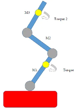
The pendulum consists of three arms that are hinged by ball bearings and can rotate in the vertical plane. The torques T1 and T2 are the

(2)

2 inputs to the pendulum with the middle hinge made free for rotation. By controlling the angles of the arms around specified values, the pendulum can be stabilized inversely with the desired angle attitudes. The triple inverted pendulum is shown in Figure 1 below.

Figure 1 the triple pendulum

Let Θi denote the angle of the ith arm measured from the vertical axis as shown in Figure 2 below.

Figure 2 System Configuration The mathematical modelling of the triple inverted pendulum is derived under the assumption that each arm is a rigid body

Lagrange differential equations is the method used to construct the triple pendulum with a

nonlinear vector-matrix differential equation of the form:

 

1

1, 2, 3 1, 2

i i i j

M N q GT

i j         Where              

1 1 2 1 2 1 3 1 3

1 2 1 2 2 2 3 2 3

1 3 1 3 2 3 2 3 3

cos cos

cos cos 2

cos cos

J l M l M

M l M J l M

l M l M J

                   _   _  _ _    Where

1 1 1 2 1 3 1 2 2 2 3 2 3 3 3

M m h m l m l

M m h m l

M m h

  

 



and

2 2 2

1 1 1 1 2 1 3 1

2 2

2 2 2 2 3 2 2 3 3 3 3

J I m h m l m l J I m h m l J I m h

   

  

 

The N matrix become:

 

1 2 2

2 2 3 3

3 3

0

3 0

C C C

N C C C C

C C       _    _  _   

And the q matrix and G matrix are

     

       

2 2

1 1 2 1 2 2 1 3 1 3 3 1 1

2 2

2 1 2 1 2 1 2 3 2 3 3 2 2

2 2

3 1 3 1 3 1 1 3 2 3 2 3 2 2 3 3 3

sin sin sin

sin 2 sin 2 sin

q l M l M M g

                                          1 0 1 1 0 1 G      _ _  _   

The description of the system is shown in Table 1 below

No Symbol Description

1 l_i length of the ith arm 2 h_i the distance from the

bottom to the centre of gravity

of the ith arm

3 m_i mass of the ith arm 4 _i angle of the ith arm from

(3)

3 5 C_i coefficient of viscous

friction of the ith hinge 6 I_i moment of inertia of the

i-th arm around the centre of

gravity

7 T_j control torque of the jth hinge

After linearization of Equation (2) under the assumptions of small deviations of the pendulum from the vertical position and of small velocities, one obtains the following equation

 4 1, 2,3

1, 2

j

i i i m

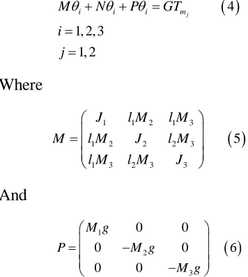
M N P GT

i j         Where   1 1 2 1 3

1 2 2 2 3

1 3 2 3 3

5

J l M l M

M l M J l M

l M l M J

     _ _   And   1 2 3 0 0

0 0 6

0 0

M g

P M g

M g     _  _  _   

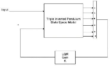
The block-diagram of the pendulum system is shown in Figure 3 and the nominal values of the parameters are given in Table 2.

Figure 3 Block-diagram of the pendulum system

Table 2 Nominal values of the parameters

No Symbol Value

1 h₁ 0.45m

2 h₂ 0.2m

3 h₃ 0.3m

4 l₁ 0.5m

5 l₂ 0.4m

6 m₁ 3.5Kg

7 m₂ 2Kg

8 m₃ 2.25Kg

9 I₁ 2

0.55Kg m

10 I₂ 2

0.12Kg m

11 I₃ 2

0.65Kg m 12 C₁ 0.07N m s 13 C₂ 0.03N m s

14 C₃ 0.009N m s

The state space representation of the triple inverted pendulum becomes

1 2 3 1 2 3

57.75 14.42 15.82 16.26 5.5 7 25.3 43 12.7 11 13.6 5 178 88.6 55.6 57.3 30.2 25 22.9 10 0.14 0.08 0.04 0.008

26 37.5 3.6 0.15 0.13 0.033 0.83 8.2 9.25 0.01 0.04 0.02

                                _ _ _ _                  1 2 3 1 1 2 2 3 1 2 3 1 2 3 1.559 0.8 4 3.8 0.65 2.4 0 0 0 0 0 0 1 0 0 0 0 0

0 1 0 0 0 0 0 0 1 0 0 0 0 0 0 1 0 0 0 0 0 0 1 0 0 0 0 0 0 1

T T y                       _         _{ }_        _{ }                    _ _{ } _ _                                   

3. The Proposed Controllers Design

3.1LQR Controller Design

(4)

4 Figure 4 Block diagram of the triple inverted

pendulum with LQR controller

In this paper, the value of Q and R is chosen as

1 0 0 0 0 0

0 1 0 0 0 0

0 0 1 0 0 0 5 0

10

0 0 0 1 0 0 0 5

0 0 0 0 1 0

0 0 0 0 0 1

Q and R

 

 

  _ _

    

 

 

 

The value of obtained feedback gain matrix K of LQR is given by

87.4053 32.8355 25.6454 27.1508 11.2981 11.1817 97.7657 45.7910 30.0834 31.2118 15.6479 12.9896

K  _

 

3.2Pole Placement Controller Design

Pole placement, is a way employed in feedback control system principle to region the closed-loop poles of a plant in pre-decided locations in the s-plane. Placing poles is proper because the region of the poles corresponds immediately to the eigenvalues of the system, which control the traits of the reaction of the system. The system ought to be considered controllable on the way to put into effect this technique. The block diagram of the triple inverted pendulum with pole placement controller is shown in Figure 5.

Figure 5 Block diagram of the triple inverted pendulum with pole placement controller

The state equations for the closed-loop system of Figure 5 can be written by inspection as

     7

x Ax Bu Ax B Kx A BK x y Cx

      



The poles for this system is chosen as





P =      1, 2, 3, 4, 5, 6

Solving using Matlab the robust pole placement algorithm gain will be

19329 8885 7472 11601 5861 6699 23483 10820 9086 14362 7268 8307

K  _

 

4. Result and Discussion

4.1Controllability and Observability

of the Pendulum

A system (state space representation) is controllable iff the controllable matrix C = [B AB A2B….An-1B] has rank n where n is the number of degrees of freedom of the system. In our system, the controllable matrix C = [B AB A2B A3B A4B A5B] has rank 6 which the degree of freedom of the system. So, the system is controllable.

(5)

5 In our system, the Observable matrix D = [C CA CA2 CA3 CA4 CA5] T has a full rank of 6. So, the system is Observable.

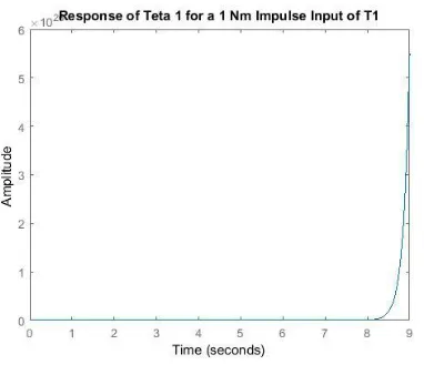
4.2Open Loop Impulse Response of

the Triple Inverted Pendulum

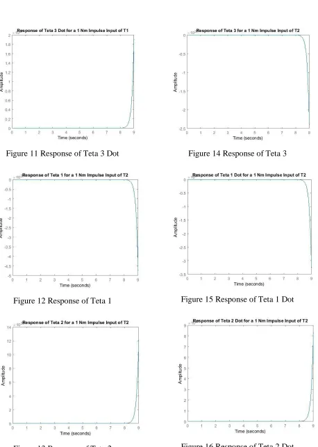
The open loop simulation for a 1 Nm impulse input of torque 1 for angular displacement 1, 2 and 3 and for angular velocity 1, 2 and 3 is shown in Figure 6, 7, 8, 9, 10 and 11 and for torque 2 input the angular displacement 1, 2 and 3 and for angular velocity 1, 2 and 3 is shown in Figure 12, 13, 14, 15, 16 and 17 respectively.

Figure 6 Response of Teta 1

Figure 9 Response of Teta 1 Dot

(6)

6 Figure 11 Response of Teta 3 Dot

(7)

As we seen from the Figures above the angular displacements and the angular velocities are unstable.

4.3Comparison of the Triple Inverted

Pendulum with LQR and Pole Placement Controllers for Impulse Input Signal

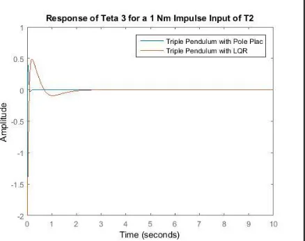
The comparison of the triple inverted pendulum with LQR and pole placement controller for a 1 Nm impulse input of torque 1 for angular displacement 1, 2 and 3 and for angular velocity 1, 2 and 3 is shown in Figure 18, 19, 20, 21, 22 and 23 and for torque 2 input the angular displacement 1, 2 and 3 and for angular velocity 1, 2 and 3 is shown in Figure 24, 25, 26, 27, 28 and 29 respectively.

(8)

Figure 23 Response of Teta 3 Dot As we seen from Figure 21, 22 and 23, for the impulse signal the angular velocities starts to increase and returns to zero for the two controllers but the pendulum with LQR controller has a high overshoot with more settling time than the pendulum with pole placement controller.

(9)

9 Figure 26 Response of Teta 3

As we seen from Figure 24, 25 and 26, for the impulse signal the angles starts to increase and returns to zero degree for the two controllers but the pendulum with LQR controller has a high overshoot with more settling time than the pendulum with pole placement controller.

As we seen from Figure 27, 28 and 29, for the impulse signal the angular velocities starts to increase and returns to zero for the two controllers but the pendulum with LQR controller has a high overshoot with more settling time than the pendulum with pole placement controller.

5. Conclusion

(10)

10 open loop simulation prove that the system is not stable without feedback control system. Comparison of the proposed controllers for an impulse input have been done and the system with pole placement controller improves the stability of the system.

Reference

[1].Mustefa Jibril et al. “Robust Control Theory Based Performance Investigation of an Inverted Pendulum System using Simulink” International Journal of Advance Research and Innovative Ideas in Education, Vol. 6, Issue 2, pp. 808-814, 2020.

[2].Ali Rohan et al. “Design of Fuzzy Logic Based Controller for Gyroscopic Inverted Pendulum System” Int. J. Fuzzy Log. Intell. Syst, Vol. 18, Issue 1, pp. 58-64, 2018.

[3].Xiaoping H. et al. “Optimization of Triple Inverted Pendulum Control Process Based on Motion Vision” EURASIP Journal on Image and Video Processing, No. 73, 2018. [4].R. Dimas P. et al. “Implementation of

Push Recovery Strategy using Triple Linear Inverted Pendulum Model in T-Flow Humanoid Robot” Journal of Physics: Conference Series, Vol. 1007, 2018.

[5].Wei Chen et al. “Simulation of a Triple Inverted Pendulum Based on Fuzzy Control” WJET, Vol. 4, No. 2, 2016.

[6].Tang Y et al. “A New Fuzzy Evidential Controller for Stabilization of the Planar Inverted Pendulum System” PLOS ONE, Vol. 11, Issue 8, 2016.