Article
Hardware in the Loop Real-Time Simulation for
Heating Systems: Model Validation and Dynamics
Analysis
Wessam El-Baz*1 ID, Lukas Mayerhofer1, Peter Tzscheutschler1ID and Ulrich Wagner1
1
2
3
4
5
6
7
8
9
10
11
12
13
14
15
16
17
1 InstituteofEnergyEconomyandApplicationTechnology,TechnicalUniversityofMunich.Arcisstr.2180333
Munich,Germany
* Correspondence:[email protected];Tel.:+49-(0)89-289-28314
Abstract: Heating systems such as heat pump and combined heat and power cycle systems (CHP)
are representing a key component in the future smart grid. Their capability to couple the electricity
and heat sector promises a massive potential to the energy transition. Hence, these systems are
continuously studied numerical and experimental to quantify their potential and develop optimal
control methods. Although numerical simulations provide time and cost-effective solution for system
development and optimization, they are exposed to several uncertainties. Hardware in the loop (HiL)
system enables system validation and evaluation under different real-life dynamic constraints and
boundary conditions. In this paper, a HiL system of heat pump testbed is presented. This system
is used to present two case studies. In the first case, the conventional heat pump testbed operation
method is compared to the HiL operation method. Energetic and dynamic analyses are performed to
quantify the added value of the HiL and its necessity for dynamics analysis. The second case, the HiL
testbed is used to validate the heat pump operation in a single family house participating in a local energy market. It enables not only the dynamics of the heat pump and the space heating circuit to be
validated but also the building room temperature. The energetic analysis indicated a deviation of 2%
and 5% for heat generation and electricity consumption of the heat pump, respectively. The model dynamics emphasized the model capability to present the dynamics of a real system with a temporal distortion of 3%
Keywords: Modelica; Heat pump; HiL; Model Validation;Testbed
18
0. Introduction
19
Installed renewable energy capacities are growing fast worldwide. At the end of 2017, 2179
20
GW were installed, with a growth rate of 8.3% during 2017 [1,2]. These capacities are expected to
21
continue growing to minimize the CO2emissions and mitigate the climate change. In Germany, several
22
legislations were introduced to create a nuclear and fossil-free economy within the framework of the
23
energy transition[3]. Among these acts are the renewable energy act, Erneuerbare Energien Gestez
24
(EEG), and the combined heat and power act, Kraft-Wärme-Kopplungsgesetz (KWKG). The EEG
25
prioritizes the renewable energy sources (RES) in the energy market [4]. It guarantees a fixed feed-in
26
tariff for the supplier to minimize the risk of the investors. Hence, the RES reached 111 GW in 2017 [4].
27
On the other hand, KWKG empowers the integration of combined heat and power (CHP) systems in
28
the national grid. A goal was set to generate 25% of the electricity by co-generation by 2020 [5]. As
29
these two acts increased the renewable energy capacities and increased the system efficiency, they
30
raised several challenges in the national grid and made the traditional grid management techniques
31
rather obsolete.
32
Sector coupling is one way to address these challenges faced by the grid. Heat pumps and CHP
33
systems are the key drivers behind the electricity and heat sectors coupling. The attractive costs
34
and lifespan of heat storages enable these heating systems to be more economically feasible to offer
35
flexibility and mitigate the fluctuating RES. Furthermore, the continuous improvement of the heat
36
pumps coefficient of performance (COP) over the past decades [6] led to a significant decrease in the
37
operation and maintenance costs. On the other hands, CHP systems are available in the markets at
38
multiple scales to serve different the utility and prosumers.
39
Given these heating systems potential in the current and future national energy system, several
40
researchers modeled and studied these heating systems [7–11]. Although the presented heating system
41
models can predict to a good extent the energy generation or consumption of a real-system, they are
42
exposed to several uncertainties as they are designed to be integrated into larger models under specific
43
system constraints. Hence, testbeds and field tests were used to investigate the quality of the result
44
and analyze the real-life system dynamics.
45
Hardware in the loop (HiL) is an approach to simulate and evaluate thermal system dynamics
46
under multiple environmental constraints. The fundamental idea of the HiL is to integrate real
47
hardware in a simulation loop. Real hardware replaces mathematical model of a system to study
48
and evaluate the quality of a developed control or optimization algorithm [12]. Hardware can also
49
be integrated with multiple numerical models to investigate its reaction to model combinations. As
50
an example, a HiL system of a heat pump as hardware and a controller as software can be used to
51
evaluate the quality of the control system. Also, a building model can be integrated to show the heat
52
pump dynamics and reaction to different building types, ages, or sizes.
53
In the literature, HiL simulation is being used in several fields. According to [12,13], it has been
54
used for over 50 years. An early application was in the flight and missiles control industry as in
55
the Sidewinder program in 1972 [14]. It has also become more popular in other industries. As an
56
example, HiL represents nowadays a crucial tool in the automotive industry [13,15]. It is extensively
57
used for engine and suspension systems control and design. Moreover, Hil is used also for testing
58
unmanned aerial vehicles as in [16]. In the electrical power sector, applications of HiL for testing and
59
validating are growing. [17] used a HiL system to study the dynamic performance of a switch-mode
60
power amplifier. In [18] a power HiL system was introduced and used to evaluate a case study of a
61
Great Britain network. [19] implemented a HiL system to investigate and compare the performance of
62
multiple control techniques for Single-Ended Primary Inductance converter(SEPIC). [20] investigated
63
different energy management strategies with electric vehicles using a HiL system in real-time. The
64
author’s setup facilitated the evaluation of the effectiveness of the design EMS strategies in real-time.
65
Furthermore, [21] designed a HiL system for water electrolysis system emulation. Through this system,
66
the author was able to study the electrolyzer characteristics in a smart grid. In [22], voltage control
67
coordination scenarios were validated based on a HiL system. The authors used HiL in a real-time
68
simulation to validate the capability of RES to provide voltage control in a smart grid.
69
Although several publications are available for power HiL systems, a limited number of
70
publications are discussing the heating systems in buildings. Among these publications is the work of
71
[23], where a HiL simulation system was developed to evaluate the control strategies of a hydronic
72
radiant heating system. The author replaced the model of the hydronic network with real hardware
73
to minimize the results uncertainties. In [24], a HiL system was developed to simulate micro-CHP
74
systems with different building models. The author showed the necessity of a HiL system in the
75
operation of micro-CHP testbeds and evaluation of optimization and control algorithms.
76
At the Institute of energy economy and application technology (IfE), several testbeds were
77
developed to evaluate all the common heating systems at different scales as in [25–27] and recently
78
in [28]. A testbed is necessary to demonstrate and validate the novel optimization algorithms and
79
control strategies being developed. Through these testbeds the operational requirements and technical
80
constraints were easily defined. Ideally, a heating system testbed should be able to demonstrate and
81
emulate a real building with a heating system and is expected to eliminate all the uncertainties, as real
hardware is used. However, as the buildings are emulated by heat sinks, uncertainties can emerge
83
and the building dynamics in certain cases diminish. The HiL systems developed at the IfE presented
84
in [24] showed the preliminary results, the potential of the HiL system, and basic evaluation of the
85
uncertainties that can emerge during the simulation. Using the recent advanced HiL version of [24],
86
the testbed in [28]and model presented in [29], the following aspects are demonstrated:
87
• A comparison between heating systems testbeds operation with HiL and without HiL system
88
simulation
89
• An energetic and dynamics analysis to quantify the benefits of HiL simulation with heating
90
systems
91
• A model validation of the heat pump dynamics and interactions within a microgrid in an energy
92
market.
93
The structure of the paper is as follows: Section1shortly describes the different numerical and
94
experimental methods used to analyze a heating system. Section2demonstrates the HiL system
95
structure including the testbed and the building model. Moreover, it presents the input system
96
parameters. Section 3demonstrates and discusses the results of the two cases discussed in this
97
publication. Section4presents a conclusive summary of the whole study.
98
1. Heating Systems Analysis Methods
99
Numerical simulation provides the ideal environment for testing and evaluation of a heating
100
system performance connected to different buildings types. Compared to experimental testing, it
101
saves efforts, costs and time to investigate a specific heating system. However, it is exposed to several
102
uncertainties, and its accuracy is questionable. Hence, experimental evaluation has always an edge
103
over the numerical simulation as it eliminates the modeling uncertainties.
104
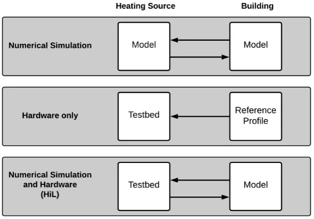
Figure 1.Abstract diagram of different methods for heating system analysis
The experimental testing can only be performed using hardware, or hardware and numerical
105
models as HiL. Figure1presents an abstract comparison between heating system analysis using
106
numerical simulation, hardware only (without HiL), and hardware and models (HiL). The conventional
107
method to evaluate the heating system experimentally is using hardware only. A reference profile that
is obtained within a field test or by a simulation model is fed directly to the testbed. This reference
109
profile contains the thermal load of the buildingPthover a specific period of time. The testbed hydraulic
110
circuit emulates this load profile using a heat sink to evaluate the reaction of the heat source and heat
111
storage. Although the heating source such as a heat pump or a micro-CHP system is a real system,
112
the results of the whole experiment are exposed to uncertainties because of the heat sink emulation of
113
the reference load profile. The heat sink always tries to reach the set reference profile, even if it has
114
to decrease the return temperature to or below the room temperature. As a conventional alternative
115
solution, return temperature can be held constant, yet it diminishes the dynamics of the whole testbed
116
operation.
117
A combination of hardware and numerical simulation is considered ro be the optimal method for
118
heating systems analysis and models validation. The heating source and heat storage are integrated as a
119
hardware with a building model using a HiL system to evaluate and validate heating systems dynamics
120
and performance. Consequently, the building model can calculate realistic return temperatures and
121
the feedback of the building for any violation introduced by the heating source. Furthermore, the
122
room temperature can be simulated by the building model. Hence, the user comfort can be analyzed
123
in real-time.
124
2. HiL Simulation System
125
2.1. Communication Structure
126
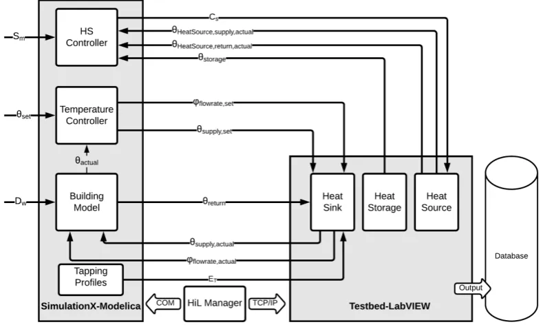
Figure2shows the detailed control loop of the implemented HiL model. The heat pump (HP)
127
controller, temperature controller, building model, and the tapping profiles are implemented on
128
SimulationX, which is a Modelica based software. More details about the models are explained later in
129
this section. The testbed, the hardware, is presented by three modules: heat sink, heat storage, and heat
130
source, which are the typical components of a heating system testbed. A LabVIEW program controls
131
the different components of the testbed and feeds the output to the database.
132
The communication between the model in SimulationX and LabVIEW is managed by the HiL
133
manager, which is based on a Matlab Code. The data is transferred between the HiL manager and the
134
LabVIEW based on the TCP/IP protocol, while a COM interface is used to manage the SimulationX
135
simulation. The details of the HiL manager communication protocols and steps are thoroughly
136
documented in [24].
137
Other communication systems were tested such as exporting the building models in the C
138
programming language (C-code) and importing the model in LabVIEW. However, processing the
139
C-code in real-time desynchronize the LabVIEW real-time control. Moreover, the number of inputs and
140
outputs to and from the C-code are limited. Hence, using C-code for integrating models in real-time
141
LabVIEW control systems is not be feasible for heating systems applications, given the size of C-code
142
and the number of communicated variables.
143
The communicated data between the testbed and the SimulationX models is dependent on the
144
functionality of the model and testbed module. The HS controller receives the actual heat source
145
supply temperatureθHeatSoruce,supply,actual, actual heat source return temperatureθHeatSoruce,return,actual,
146
and temperature of the storageθstoragefrom the testbed. Moreover, it receives an external control
147
input signalSmthat is developed from the model described in [29]. Based on these input signals,
148
the HS controller sends a binary operation signalCs to the testbed heat source. The temperature
149
controller receivesθsetandθactual, which are the set room temperature and the actual room temperature,
150
respectively. Based on these two inputs, the temperature controller can calculate the set flow rate
151
ϕf lowrate,set, and the set space heating supply temperature of the θsupply,set. The building model
152
receives the weather dataDw, actual flow rateϕf lowrate,actual, and the actual supply temperature of
153
the space heatingθsupply,actual. Based on these inputs and the building model, the return temperature
154
can be calculated and forwarded to the testbed. Communicating theθreturneach second in this HiL
155
simulation system maximizes the results accuracy and enables the testbeds to present realistic dynamics
156
that is comparable to field measurements. Tapping profiles can also be integrated as a model and
157
communicated as energy profilesETto the heat sink.
158
2.2. Testbed Components and description
159
The testbed system consists of three modules and a brine water heat pump with a thermal power
160
of 10.31 kW and a COP of 5.02 by B0/W35 as per standard EN14511. Two circulations pumps are
161
integrated into the heat pumps on the brine and the water side. Moreover, it is equipped with an
162
emergency electrical heater of 8.8 kW. Figure3shows the simplified hydraulic schematic of the used
163
testbed.
164
Having a ground-source heat pump, an emulator is needed to show the dynamics of the ground
165
heat exchanger. Module A includes a ground-source emulator that can emulate any required brine
166
temperature supplied to the heat pump. It consists of a 300-liter heat storage, filled with a water-glycol
167
mixture as an anti-freezing heat transfer fluid. The storage is heated by a 12.5 kW electrical heater that
168
is controlled via a hysteresis regulator to maintain the tank temperature during the whole operation
169
time at 40◦C. The set temperature of the tank and the hysteresis bandwidth can be defined by the user
170
depending on the simulation goals. A mixer, similar to the conventional space heating mixers, is used
171
to mix the supply of brine tank with the return of the heat pump to reach the required ground-source
172
set temperature. Depending on the HiL system and the goal of the simulation, the mixer can maintain
173
a constant brine temperature or a time-dependent temperature profile.
174
Module B shows the combi-storage system of a conventional residential house. It includes a
175
749-liter combi hygienic buffer storage to cover the space heating and domestic hot water consumption.
176
A stainless steel heat exchanger extracts heat from the storage to cover the hot water consumption.
177
Moreover, a coaxial pipe, pipe-in-pipe system, is used to enable the hot water and maintain the pipe
178
temperatures at a certain level.
179
Module C is the most complex module as it represents the heat sink of the testbed. It can emulate
180
the space heating and domestic hot water consumption depending on the building type and user
181
behavior. The space heating circuit consists of a space heating mixer, circulation pump, and two heat
182
exchangers. Through the mixer, the supply of the tank with the return of the space heating is mixed
183
to reach the requiredθsupply,set. The circulation pump is controlled depending onϕf lowrate,set, which
184
varies depending on the heat demand. Two heat exchangers of two different sizes are used to emulate
185
different building loads depending on their required maximum heat power. The domestic hot water
186
consumption is emulated through three magnetic valves that have different consumption flow rates.
187
These valves can represent different consumption activities such as washing, showering or cooking.
188
The hydraulic configuration in figure 3 shows only one of the most common hydraulic
189
configuration. However, the testbed can allow several other configurations, such as the direct
190
connection of the heat pump to module C, or using an additional heat storage for hot water
191
consumption. More details about the hydraulics, control and dynamics of the testbed are available in
192
[28].
193
2.3. Models Description
194
Earlier in [29], a market model is presented based on a double-sided auction, in which different
household devices and heating systems can participate. The heat system bids their energy needs to either minimize their costs, maximize comfort, or local generation in a microgrid. In this paper,
the market control approach is going to be used to develop the external control signal, Sm. The
control signal provided in this case is a binary signal, either 0 or 1. The HS controller reacts to the
signal as in equation1, whereθHeatSource,supply,maxis the maximum heat source supply temperature,
θHeatSource,return,maxis the maximum heat source return temperature, andθstorage,maxis the maximum storage temperature at a specified sensor position.
CS =
0, ifθHeatSource,supply,actual≥θHeatSource,supply,max,
0, ifθHeatSource,return,actual≥θHeatSource,return,max,
0, ifθstorage≥θstorage,max,
Sm, otherwise
(1)
TheSmis considered in full control, yet the HS has to make sure that the heat source operation never
195
exceeds the operation limit set by the manufacturer.
196
The temperature controller sets the flow rate and supply temperature of the heating circuit. The
flow rate is determined based the room actual temperatureθactualand set temperatureθset, while the
the temperature controller operates based on a hysteresis algorithm. The set flow rate of the heating
circuitϕf lowrate,setis calculated based onθactual−θset,∆+r , and∆−r where∆r+and∆r−are the hysteresis
upper and lower limits, respectively. These limits are determined by the user depending on the level
of comfort required. The smaller the absolute value of∆+r and∆−r , the higher comfort. Equation2
details the control cases of the flow rate.
ϕf lowrate,set=
ϕf lowrate,min, ifθactual−θset>∆+r , ϕf lowrate,max, ifθactual−θset<∆−r ,
ϕf lowrate,max−ϕf lowrate,min
∆+ r −∆−r
×(θactual−θset) +ϕf lowrate,min, otherwise
(2)
The supply temperature is determined based on the outside temperature given inDw. The supply
197
temperature varies linearly against the outside temperature. The lower the outside temperature, the
198
higher is the supply temperature of the space heating system. The limits and the magnitude of this
199
linear relationship between the outside temperature and the heating system supply temperature is
200
defined based on the age of the building and the type of the radiators. In section2.4, the used supply
201
temperature curve is explained.
202
2.4. Model Input Data and Parameters
203
The building model is created and calibrated based on the research project data of [30]. It consists
204
of three heated zones to represent an Attic, a living area and a cellar. The base model is available in the
205
Green City package of SimulationX [31]. The construction year of the building is between 1984 and
206
1994. The living area has 150 square meters and a room height of 2.5 meters. The cellar and attic are
207
unheated. The living area is heated and the temperature is maintained at 21◦C. In table1, a summary
208
of the most important input data parameters are presented.
209
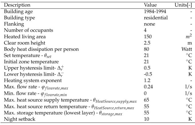
Table 1.Building and control models basic parameters
Description Value Units[-]
Building age 1984-1994
-Building type residential
-Flanking none
-Number of occupants 4
-Heated living area 150 m2
Clear room height 2.5 m
Body heat dissipation per person 80 Watt
Set temperature -θset 21 ◦C
Initial zone temperature 21 ◦C
Upper hysteresis limit-∆+r 0.5 K
Lower hysteresis limit-∆−r -0.5 K
Heating system exponent 1.2
-Max. flow rate -ϕf lowrate,max 0.24 l/s
Min. flow rate -ϕf lowrate,min 0 l/s
Max. heat source supply temperature -θHeatSource,supply,max 65 ◦C Max. heat source return temperature -θHeatSource,return,max 55 ◦C Max. storage temperature (lowest layer) -θstorage,max 55 ◦C
Night setback 10 K
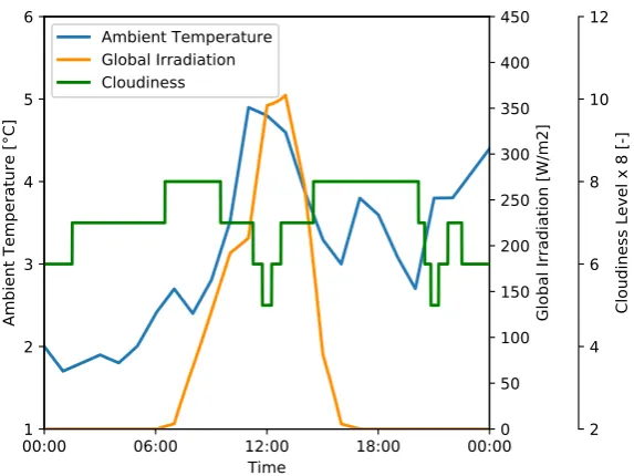
A winter cloudy type day is selected based on the VDI Standard 4655. The ambient weather
210
temperature, the global solar irradiation, and the cloudiness are shown in figure4. According to the
211
standard, the average temperature should be below 5◦C and the cloudiness should be higher than 5/8.
212
On the selected day, the average temperature and cloudiness was 3.15◦C and 7/8, respectively. The
213
number of cloudy winter days in the reference year was 85 days. The presented profile represents a
214
typical average day of the given year in Munich Germany. A winter type day is chosen to show clearly
the influence of HiL on the quality of the results. A summer type day could have been selected, yet
216
the space heating circuit would not be activated in this case. Hence, the HiL influence would not be
217
noticed.
218
00:00
06:00
12:00
18:00
00:00
Time
1
2
3
4
5
6
Ambient T
emperature [°C]
0
50
100
150
200
250
300
350
400
450
Global Irradiation [W/m2]
Ambient Temperature
Global Irradiation
Cloudiness
2
4
6
8
10
12
Cloudiness Level x 8 [-]
Figure 4.A winter cloudy type day temperature and global irradiation
The heating circuit supply temperature is defined according to equation3, whereθais the ambient
temperature. As shown, the supply temperature varies depending on the outside ambient temperature. The slope of the supply temperature is defined according to the recommended operation constraints and the nature of the building itself. Moreover, the required set temperature and required user comfort level can play an important role in deciding the slope of the heating curve. A change in the set temperature or the comfort level can be accompanied by a parallel shift of the heating circuit supply curve. To increase the comfort and the decrease the time required to reach the set temperature, parallel upwards shift can be made. On the other hands, if the user needs to decrease the costs, the heating curve can be shifted downwards.
θSupply,set =
50, ifθa<−20
−0.625×θa+37.5, if −20≤θa≤20,
25, ifθa>20
(3)
3. Results and Analysis
219
In this paper, two cases are evaluated. The first case compares the testbed operation with and
220
without HiL to present the added value and necessity of the HiL system. The comparison is based on
221
energetic and dynamics analysis of the two experimental methods. The energetic analysis compares the
222
energy consumption of the heat source and heat sink within the period of time depending on the given
223
type day in section2.4. The dynamic analysis investigates and compares power and temperatures over
224
time of the two testbed experiments with and without HiL and discusses its impact on the heating
225
system evaluation.
226
In the second case, the HiL system is used to validate a single family house model with a heat
227
pump participating in an energy market. Preliminary market model was presented in [29]. The system
228
dynamics evaluation of the model is crucial as it influences the time, volume and price of the heat
pump energy asked from the market. Hence, a comparison is conducted between the HiL system and
230
the model to evaluate and demonstrate the model accuracy.
231
3.1. Case 1: Testbed Operation With and Without HiL
232
In this case, the testbed operation with and without HiL is compared to quantify the added value
233
and present the necessity of the HiL system. A reference load profile is generated from the building
234
model and type day presented in section2.4. The building model is connected to an over-sized heating
235
source or a district heating to simulate the exact heat demand profile of the building without any
236
compromises on the comfort side of the user.
237
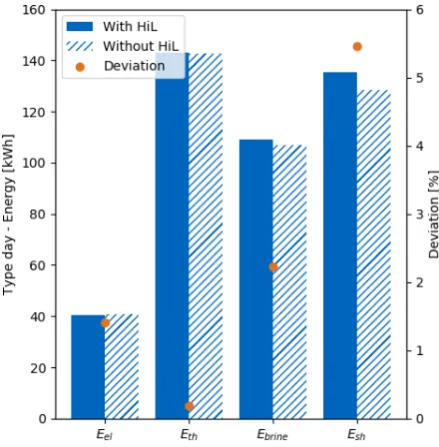
Figure 5.Energetic analysis of the testbed performance with and without HiL
Figure5presents the energy consumption and generation of the type day experiment, where
238
Eelis the electric energy consumption of the heat pump,Ethis the thermal energy generation of the
239
heat pump,Ebrineis the energy consumed from the brine side, andEsh is the energy consumed by
240
the building. It can be seen that the deviation is between 0.2% to 5.5%, which is not significantly
241
large. However, it can be noticed that using the same metrics, the operation without HiL always
242
has a lower consumption than the one with HiL. The reference space heating profile consumption
243
is 132.8 kWh, compared to 135.3 kWh for the operation with HiL and 128.4 kWh for the operation
244
without HiL. Although the experiment with HiL system is closer to the reference, it does not indicate a
245
significant failure in the experiment without HiL. Hence, operating heating system testbeds without a
246
HiL communication system has been widely accepted over the past years.
247
Insight on the dynamics and the difference between the testbed operation with and without HiL
248
can be presented in figure6. Although the energy consumption is almost equal, a significant difference
249
can be seen in the space heating dynamics between the operation with HiL, without HiL and the
250
reference profile. Between 00:00 and 06:00 in figure6(a), no differences can be noticed. The testbed
251
operations are identical to the reference profile. With the increasing demand after 06:00 and the lack of
252
sufficient energy in the heat storage, the power dropped. The testbed operation without HiL reaction
253
is to reduce the return temperature trying to maintain the same power, as in figure6(b). The return
254
temperature in this case decreases to 17◦C, which shows a major violation as the return temperature is
255
lower than the room temperature. The testbed would have decreased the return temperature even
256
to a lower level than 17◦C, but it is constrained by the cooling circuit. On the other hand, the HiL
system maintained a plausible return temperature due to the integration of a building model in the
258
loop. Moreover, the HiL increased the power after 08:00 to make up for the power drop started at 06:00
259
and maintain a proper temperature, while the testbed operation without continued to maintain the
260
reference profile.
261
00:00 06:00 12:00 18:00 00:00 Time
0 2 4 6 8 10 12
Power
[kW]
SH-Thermal Power-With HiL SH-Thermal Power-Without HiL SH-Thermal Power-Reference Profile
(a)
00:00 06:00 12:00 18:00 00:00 Time
15 20 25 30 35 40 45 50 55
Temperature [°C]
SH-Supply-With HiL SH-Supply-Without HiL SH-Return-With HiL SH-Return-Without HiL
(b)
Figure 6.Comparison between the space heating dynamics of the testbed operation with HiL and without HiL against the reference profile, (a) space heating thermal power, (b) space heating supply and return temperatures
Another drop in power can be noticed between 12:00 and 18:00 for the HiL system. The testbed
262
operating without HiL maintained the reference load profile power, even though there were not
263
sufficient amount of energy in the storage. This can be confirmed by the decrease in supply temperature
264
noticed in figure6(b). This drop is due to incapability of the heat pump to meet the demand. The
265
HiL maintained a plausible return temperature, but return temperature without the HiL decreased
266
significantly. Although the power of the testbed operation without HiL seems acceptable, the return
267
temperature dynamics are not realistic and can not be relied on for model validation or further research.
268
00:00 06:00 12:00 18:00 00:00 Time
0 2 4 6 8 10 12 14 16
Power [kW]
HP-Thermal Power-With HiL HP-Electrical Power-With HiL HP-Thermal Power-Without HiL HP-Electrical Power-Without HiL
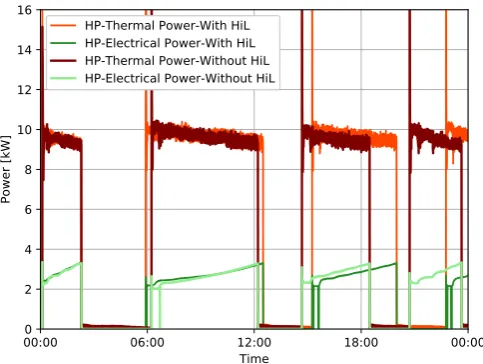
Figure 7.Thermal and electrical power of the heat pump with and without HiL
The energetic analysis shows almost an identical energy consumption and generation behavior of
269
the heat pump system, yet the system dynamics shows the necessity of a HiL system. The behavior of
the space heating circuit led to another operation plan for the heat pump, although it uses the same
271
controller strategy. As in figure7, the heat pump started at the same time and behaved similarly within
272
the first operation cycle. With the second cycle starting at 06:00, a difference between the two cycles
273
can be seen. This difference is increasing over time as seen at 15:00 and again at 20:00. This difference
274
between the two systems can lead to a significant error in the evaluation of energy management
275
systems using heat pumps and cost optimization models based on variable electricity tariffs, or in
276
energy markets as discussed later in section3.2. The exact operation plan represents a necessity in
277
evaluating and validating the flexibility potential of heat pumps.
278
3.2. Case 2: Model Validation Based on HiL
279
Based on the model presented in [29], 10 single family residential houses are simulated located in
280
Munich, Germany. These houses are participating in a local energy market, where each device sell or
281
buy energy depending on its operation mode. Each house is equipped with a photovoltaic system,
282
an electric vehicle and a heat pump. The installed PV capacity at each house is 6 kWp. The technical
283
details and the data of the integrated PV system can be found in [32]. A 3.6 kW charging station is
284
used for the electric vehicle, while the integrated heat pump is represented by the testbed in section
285
2.2. More details about the heat pump testbed can be found in [28]. A single family house is selected
286
from these 10 houses to be validated based on the HiL system and the heat pump testbed.
287
00:00 06:00 12:00 18:00 00:00 Time
0 2 4 6 8 10 12
Power [kW]
SH-Thermal Power-With HiL SH-Thermal Power-Simulation
(a)
00:00 06:00 12:00 18:00 00:00 Time
15 20 25 30 35 40 45 50 55
Temperature [°C]
SH-Supply-With HiL SH-Supply-Simulation SH-Return-With HiL SH-Return-Simulation
(b)
00:00 06:00 12:00 18:00 00:00 Time
20.70 20.75 20.80 20.85 20.90 20.95 21.00 21.05 21.10
Temperature
[°C]
Room Actual Temperature - HiL Room Actual Temperature - Simulation
(c)
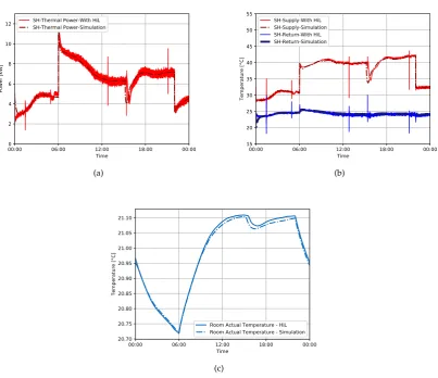
The goal of the model validation is to compare the operation of the heat pump in the model to
288
the testbed with HiL, while making sure that the building load is covered and the room temperature
289
is properly maintained. On the heat sink side, figure8(a)shows that the space heating power of the
290
testbed with HiL and the simulation are behaving similarly, even when a drop in the storage energy
291
occurred at 17:00. This drop did not influence the room temperature as shown in figure8(c). The room
292
temperature of the complete simulation model and the building model within the HiL system are
293
behaving similarly. A difference can be noticed from 09:00 to 22:00, yet this difference is below 0.02
294
◦C. In figure8(b), the supply and return temperature of the HiL testbed and simulation model can
295
be compared. It can be noticed that the return temperatures are not violated and both the HiL and
296
simulation are behaving similarly except at the starting point, where a minor fluctuation occurred by
297
the simulation solver.
298
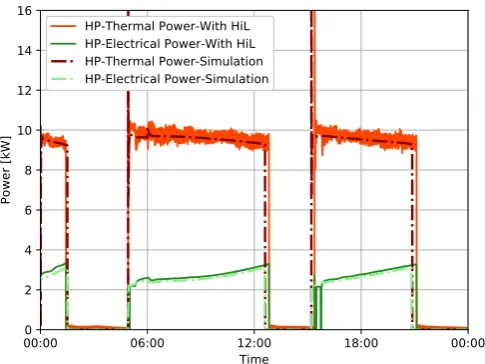
The behavior of the heat pump in the HiL and simulation is almost identical as in figure9. The
299
power magnitude of the thermal and electrical power is equivalent, which means that the heat pump
300
has been providing power to the heat storage almost at the same supply temperature. In this type day,
301
the energy difference between the HiL system and the simulation is 2% and 5% for the heat generation
302
and electricity consumption, respectively. However, the HiL based validation in this paper is not only
303
concerning the energetic consumption but also the temporal distortion of the power. The time and
304
volume of the heat pump bid in an energy market have to be evaluated to validate the accuracy of the
305
heat pump bid in the market.
306
00:00 06:00 12:00 18:00 00:00 Time
0 2 4 6 8 10 12 14 16
Power [kW]
HP-Thermal Power-With HiL HP-Electrical Power-With HiL HP-Thermal Power-Simulation HP-Electrical Power-Simulation
Figure 9.Heat pump thermal power and electrical power on the type day
In [28], the thermal and electrical power of the heat pump model were validated independently
307
based on mean absolute percentage error (MAPE) and root mean square error (RMSD). However, since
308
the temporal distortion of the model compared to the HiL is crucial to evaluate the model capability in
309
participating in local energy markets at the estimated times, the temporal distortion index (TDI) of
310
[33] is used. This metric is based on the dynamic time warping (DTW) developed in the 70s, which is
311
used to evaluate the temporal distortion between two different time series. In this paper, the two time
312
series are the HiL measurement and simulation model time series of the heat pump electrical power.
313
The DTW finds the optimal path through minimizing the distance between the two given time series.
314
Then, it returns the optimal warping path given the simulation model output with the indexi, the HiL
315
measurements with the indexj, and the smallest distance between them. The TDI is calculated then
316
according to equation4.
TDI= 1 N2
k−1
∑
l=1|(il+1−il)(il+1+i1−jl+1−jl)| (4)
The output of the TDI is between 0 and 1. The lower the value of the TDI metric, the lower is the
318
temporal distortion. The metric result in this type day is 3%, which means that the simulation model
319
and the HiL have a low temporal distortion.
320
4. Conclusion
321
In this paper, hardware in the loop (HiL) real-time system is presented. The HiL communication
322
structure, models and testbeds are explained to show the experimental setup of HiL for heating systems.
323
The testbed of a ground source heat pump (GSHP) demonstrated in [28] is used as a candidate for this
324
study. To evaluate the potential and applications of the HiL, two case studies are discussed. The first
325
case study evaluates the energy consumption and the dynamics of the testbed operation with and
326
without HiL. The results of the case study are summarized as follows:
327
• Testbed operation with or without HiL does not influence the energy consumption of the heat
328
sink (space heating), or the heat generation from the heat pump. The variations in results are
329
between 0.2% and 5.5%. Hence, energetically no significant difference can be noticed
330
• The dynamics of the testbed operation without HiL showed that a drop in the space heating
331
supply temperature is always accompanied with a drop in the return temperature of the space
332
heating. Thus, testbed operation without HiL can not emulate real-life return temperature
333
dynamics and can lead to system violations
334
• The HiL system is able to maintain realistic dynamics due to the availability of a building model
335
in the loop
336
• The violations of the testbed operation without HiL led to a shift in the operation plan of the
337
heat pump. Hence, the testbed operation without HiL is not reliable for heating system models
338
validation
339
In the second case, the HiL system was used to validate a single family house building
340
participating in a local energy market. The HiL system was chosen as it was necessary to validate not
341
only the energy consumption but also the system dynamics and the temporal distortion of the model.
342
The simulation model showed its capability to present the heat pump system dynamics including any
343
drops in the supply temperature or the heat storage of the tank. The HiL also showed an advantage of
344
demonstrating the room temperature of the building model for the given type day, which facilitates
345
evaluating the comfort of the residents and comparing it to the simulation model. Furthermore, TDI
346
is used to quantify the temporal distortion of the heat pump to make sure that the electric energy
347
consumption is communicated at the right time of the day. The TDI value is 3%. Hence, a minimal
348
temporal distortion can be noticed between the HiL and the simulation model.
349
As an outlook, HiL for heating systems can be used for several further studies. It enables not only
350
an accurate validation of simulation model but also experimentation using the building model inertia
351
to offer flexibility to the grid. The HiL can also include not only one heating system or a building
352
model, but also multiple heating systems that can communicate and interact in the same local heating
353
network or a microgrid.
354
5. Acknowledgment
355
This work was supported by the German Research Foundation (DFG) and the Technical University
356
of Munich within the Open Access Publishing Funding Program. The research project is supported by
357
the Federal Ministry for Economic Affairs and Energy, Bundesministerium für Wirtschaft und Energie,
358
as a part of the SINTEG project C/sells. Responsibility for the content of this publication lies on the
359
authors.
6. Author Contributions
361
Wessam El-Baz designed the experiments and developed the HiL system. Lukas Mayerhofer
362
operated the testbed and prepared the energetic analysis. Peter Tzscheutschler and Ulrich Wagner
363
provided a detailed critical review. All the authors discussed the documents results and contributed to
364
the preparation of the manuscript.
365
7. Conflicts of Interest
366
The authors declare no conflict of interest
367
References
368
1. IRENA International Renewable Energy Agency. Renewable capacity highlights2018. p. 2. 369
2. Capuano, L. International Energy Outlook 2018 (IEO2018)2018. 2018, 21. 370
3. Renewable Energies Agency. Press Fact Sheet: The German Energy Transition. Berlin Energy Transition 371
Dialogue2016, pp. 1–16.
372
4. Federal Republic of Germany. Act on the Development of Renewable Energy Sources - RES Act 20172017. 373
p. 179. 374
5. German Ministry of Economics and Energy. BMWi - Kraft-Wärme-Kopplung. 375
6. Haller, M.Y.; Haberl, R.; Mojic, I.; Frank, E. Hydraulic integration and control of heat pump 376
and combi-storage: Same components, big differences. Energy Procedia 2014, 48, 571–580. 377
doi:10.1016/j.egypro.2014.02.067. 378
7. Bloess, A.; Schill, W.P.; Zerrahn, A. Power-to-heat for renewable energy integration: A review of 379
technologies, modeling approaches, and flexibility potentials. Applied Energy 2018, 212, 1611–1626. 380
doi:10.1016/j.apenergy.2017.12.073. 381
8. Braun, J.; Bansal, P.; Groll, E. Energy efficiency analysis of air cycle heat pump dryers.International Journal 382
of Refrigeration2002,25, 954–965. doi:10.1016/S0140-7007(01)00097-4.
383
9. Willem, H.; Lin, Y.; Lekov, A. Review of energy efficiency and system performance of residential heat 384
pump water heaters.Energy and Buildings2017,143, 191–201. doi:10.1016/j.enbuild.2017.02.023. 385
10. Badache, M.; Ouzzane, M.; Eslami-Nejad, P.; Aidoun, Z. Experimental study of a carbon dioxide 386
direct-expansion ground source heat pump (CO2-DX-GSHP). Applied Thermal Engineering 2018, 387
130, 1480–1488. doi:10.1016/j.applthermaleng.2017.10.159. 388
11. Ikeda, S.; Choi, W.; Ooka, R. Optimization method for multiple heat source operation including ground 389
source heat pump considering dynamic variation in ground temperature.Applied Energy2017,193, 466–478. 390
doi:10.1016/j.apenergy.2017.02.047. 391
12. Bacic, M. On hardware-in-the-loop simulation. Proceedings of the 44th IEEE Conference on Decision and 392
Control2005, pp. 3194–3198. doi:10.1109/CDC.2005.1582653.
393
13. Bonvini, M.; Donida, F.; Leva, A. Modelica as a design tool for hardware-in-the-loop simulation2009. pp. 394
378–385. doi:10.3384/ecp09430087. 395
14. Bailey, M. Contributions of hardware-in-the-loop simulations to Navy test and evaluation. Proceedings of 396
SPIE. SPIE, 1996, Vol. 2741, pp. 33–43. doi:10.1117/12.241122. 397
15. Winkler, D.; Gühmann, C. Hardware-in-the-Loop simulation of a hybrid electric vehicle using 398
Modelica/Dymola. 22nd International Battery, Hybrid and Fuel Cell Electric Vehicle Symposium2006, pp. 399
1054–1063. 400
16. Kamali, C.; Jain, S. Hardware in the Loop Simulation for a Mini UAV.IFAC-PapersOnLine2016,49, 700–705. 401
doi:10.1016/j.ifacol.2016.03.138. 402
17. Sun, J.; Yin, C.; Gong, J.; Chen, Y.; Liao, Z.; Zha, X. A stable and fast-transient performance 403
switched-mode power amplifier for a power hardware in the loop (PHIL) system. Energies2017,10. 404
doi:10.3390/en10101569. 405
18. Guillo-Sansano, E.; Syed, M.H.; Roscoe, A.J.; Burt, G.M. Initialization and synchronization of 406
power hardware-in-the-loop simulations: A Great Britain network case study. Energies 2018, 11. 407
19. Rosa, A.; de Souza, T.; Morais, L.; Seleme, S. Adaptive and Nonlinear Control Techniques Applied to 409
SEPIC Converter in DC-DC, PFC, CCM and DCM Modes Using HIL Simulation. Energies2018,11, 602. 410
doi:10.3390/en11030602. 411
20. Castaings, A.; Bouscayrol, A.; Lhomme, W.; Trigui, R. Power Hardware-In-the-Loop simulation for testing 412
multi-source vehicles. IFAC-PapersOnLine2017,50, 10971–10976. doi:10.1016/j.ifacol.2017.08.2469. 413
21. Ruuskanen, V.; Koponen, J.; Sillanpää, T.; Huoman, K.; Kosonen, A.; Niemelä, M.; Ahola, J. Design and 414
implementation of a power-hardware-in-loop simulator for water electrolysis emulation.Renewable Energy 415
2018,119, 106–115. doi:10.1016/j.renene.2017.11.088. 416
22. Shahid, K.; Petersen, L.; Olsen, R.; Iov, F. ICT Based HIL Validation of Voltage Control Coordination in 417
Smart Grids Scenarios. Energies2018,11, 1327. doi:10.3390/en11061327. 418
23. Rhee, K.N.; Yeo, M.S.; Kim, K.W. Evaluation of the control performance of hydronic radiant heating 419
systems based on the emulation using hardware-in-the-loop simulation. Building and Environment2011, 420
46, 2012–2022. doi:10.1016/j.buildenv.2011.04.012. 421
24. El-Baz, W.; Sänger, F.; Tzscheutschler, P. Hardware in the Loop ( HIL ) for micro CHP Systems. The Fourth 422
International Conference on Microgeneration and related Technologies2015.
423
25. Mühlbacher, H. Verbrauchsverhalten von Wärmeerzeugern bei dynamisch variierten Lasten und 424
Übertragungskomponenten2007. p. 127. 425
26. Wehmhörner, U. Multikriterielle Regelung mit temperaturbasierter Speicherzustandsbestimmung für 426
Mini-KWK-Anlagen2012. 427
27. Lipp, J.P. Flexible Stromerzeugung mit Mikro-KWK-Anlagen, 2015. 428
28. El-Baz, W.; Tzscheutschler, P.; Wagner, U. Experimental study and modeling of ground-source heat pumps 429
with combi-storage in buildings. Energies2018,11. doi:10.3390/en11051174. 430
29. El-Baz, W.; Tzscheutschler, P. Autonomous coordination of smart buildings in microgrids based on a 431
double-sided auction. 2017 IEEE Power & Energy Society General Meeting; IEEE: Chicago, 2017; Number 432
August, pp. 1–5. doi:10.1109/PESGM.2017.8273944. 433
30. EPISCOPE. IEE Project TABULA. 434
31. ESI ITI. SimulationX 3.8 | Green City. 435
32. El-Baz, W.; Honold, J.; Hardi, L.; Tzscheutschler, P. High-resolution dataset for building energy 436
management systems applications.Data in Brief2018,54, 1–5. doi:10.1016/j.dib.2017.12.058. 437
33. Frías-Paredes, L.; Mallor, F.; León, T.; Gastón-Romeo, M. Introducing the Temporal Distortion 438
Index to perform a bidimensional analysis of renewable energy forecast. Energy 2016, 94, 180–194. 439
![Figure 3. Hydraulic schematic of the heat pump testbed [28]](https://thumb-us.123doks.com/thumbv2/123dok_us/7962748.1320838/5.595.125.466.546.736/figure-hydraulic-schematic-heat-pump-testbed.webp)