Predictive
Simulation
of
Concurrent
Debris
Flow:
How
Slope
Failure
Locations
Affect
Predicted
Damage
Kazuki YAMANOIa,b , Satoru OISHIb, Kenji KAWAIKEa, Hajime NAKAGAWAa
a: Disaster Prevention Research Institute, Kyoto University ,Shimomisu-higashinokuchi, Yoko-oji, Fushimi-ku, Kyoto ,Kyoto 6128235, Japan
b: RIKEN Center for Computational Science, 7-1-26 Minatojima-minami-machi, Chuo-ku, Kobe, Hyogo 6500047 , Japan
Corresponding author : Kazuki Yamanoi ([email protected])
[1]Disaster Prevention Research Institute, Kyoto University ,Shimomisu-higashinokuchi, Yoko-oji, Fushimi-ku, Kyoto ,Kyoto 6128235, Japan
[2]RIKEN Center for Computational Science, 7-1-26 Minatojima-minami-machi, Chuo-ku, Kobe, Hyogo 6500047 , Japan
Abstract
Predictive simulation of concurrent debris flow using only pre-disaster information has proven to be difficult as a result of problems in predicting the location of debris-flow initiation (i.e., slope failure). However, because catchment topography has concave characteristics, with all channels in a catchment joining each other as they flow downstream, it is possible to predict damage to downstream area using relatively inaccurate initiation points. Based on this, this paper presents methodologies employing debris-flow initiation points generated randomly using statistical slope failure prediction. A many-case simulation across numerous initiation points was performed to quantify the effect of slope-failure location in terms of deviations in the predicted water level and terrain deformation. It was found that the relative standard deviation diminished as the points approached the downstream area, indicating a location-based predictability effect. (131 words)
1
Introduction
Debris flow is a primary hazard to human life. When significant rainfall events impact watershed topography, multiple debris flows take place concurrently within a single catchment. A case occurred on Northern Kyushu Island, Japan, in July 2017, when heavy rains induced multiple landslides, producing debris flows in the Akatani River catchment with areas of approximately 20km2. Subsequently, massive amounts of sediment covered a residential area located at the bottom of the valley. Sediment was also transported several kilometers downstream and deposited at widths of approximately 150m through a channel with an original width of only about 10m. The sediment-laden flood damaged both channel sides and areas far from the main channels. The disaster killed 33 people, and it damaged 1,046 buildings throughout Asakura city according to the report by Fukuoka pref., Japan.
The event was remarkable in that it produced sediment from multiple landslides, which strongly affected the inundation processes. Large terrain deformation around channels caused by the flood gave severe damage to the areas outside of the hazard map.
Numerical simulation is an important method for assessing risk and designing counter-measures against debris-flow- and sediment-laden floods. Such simulation models (e.g., Naef et al. (2006); O'Brien et al. (1993); Hungr and McDougall (2009)) normally depend on theory derived from flume experiments or field investigations. By employing these techniques, reproductive debris-flow simulation is possible using post-disaster information, including field survey data such as peak discharge, area of deposition, material size, and depth of erodible soil. However, the limited availability of prior field data means that the precise risk of disaster cannot be obtained via simulation during the pre-disaster phase and, to date, no effective predictive prior-disaster simulation schemes have been developed.
Given this limitation, model simulations are typically carried out using a hydrograph that flows from the outlet of the debris-flow-prone catchment (e.g., Rickenmann et al. (2006); Nakatani et al. (2016)). In general, such hydrographs are modeled using rainfall-runoff simulation or rainfall data processing. However, the prediction of the potential scales of heavy rainfall events requires significant effort. Furthermore, because debris flow can grow by eroding and consuming bed material, the debris-flow peak discharge tends to be higher than that of floods, which can be predicted using a simple rainfall runoff simulation (Hungr et al., 2001). Thus, hydrograph-based condition-setting for debris flow simulation usually requires empirically based modification.
Focusing on landslide-induced debris flow alone enables the use of an alternative approach in which the debris flow is simulated from its initiation based on its development process (Revellino et al., 2004). This requires no assumptions regarding the rainfall-runoff process, although some assumptions regarding how the debris flow initiates at the landslide are needed. Furthermore, precise landslide data are needed to carry out the simulation. Unfortunately, precise deterministic landslide prediction is difficult using current techniques because of inequalities in underground conditions (cohesion, inside friction angle, water retention, and hydraulic conductivity) and observational difficulties in obtaining such data.
However, because watershed topography has a concave characteristic, in which tributaries aggregate as they flow downward, similar scales of debris flow can result even if the landslide initiation point changes within the catchment. This suggests that a relatively low prediction accuracy in terms of debris flow initiation location might not be unacceptable in determining the risk to downstream areas. Using this hypothesis, we could quantify the uncertainty in debris-flow initiation location by conducting a multi-case simulation in which the initiation point was varied using a statistical method.
2
Simulation
methodology
2.1
Governing
equations
To treat debris flow, we selected a two-dimensional simulation model based on the dilatant fluid model developed by Takahashi (2007), which has been frequently applied in practice (Wu et al., 2013; Nakatani et al., 2016). The governing equations can be written as
𝜕𝐔 𝜕𝑡
𝜕𝐄 𝜕𝑥
𝜕𝐅
𝜕𝑦 𝐒, (1)
where 𝑈 is the conservative variable vector, 𝐸 and 𝐹 are the flux vectors in the x- and y-directions, respectively, and 𝑆 is the source vector. This equation is the integrated form of shallow-water equations and equations for sediment transport comprising the volumetric conservation law of the fluid (debris flow), momentum equations for the x- and y-directions, the volumetric conservation law of concentration of sediment in fluid, and the land-surface material conservation law.
The vectors are defined as
𝐔 ⎝ ⎜ ⎛ ℎ 𝑢ℎ 𝑣ℎ 𝐶ℎ 𝑧 ⎠ ⎟ ⎞ ,𝐄 ⎝ ⎜ ⎜ ⎛ 𝑢ℎ
𝑢 ℎ 1
2𝑔ℎ 𝑢𝑣ℎ 𝐶𝑢ℎ 0 ⎠ ⎟ ⎟ ⎞ ,𝐅 ⎝ ⎜ ⎜ ⎛ 𝑣ℎ 𝑢𝑣ℎ
𝑣 ℎ 1
2𝑔ℎ 𝐶𝑣ℎ 0 ⎠ ⎟ ⎟ ⎞ , 𝐒 ⎝ ⎜ ⎜ ⎜ ⎜ ⎛ 𝑖 𝑔ℎ 𝑆 𝑆 𝜕 𝜕𝑥 𝜖 𝜕 𝑢ℎ 𝜕𝑥 𝜕 𝜕𝑦 𝜖 𝜕 𝑢ℎ 𝜕𝑦 𝑔ℎ 𝑆 𝑆 𝜕 𝜕𝑥 𝜖 𝜕 𝑣ℎ 𝜕𝑥 𝜕 𝜕𝑦 𝜖 𝜕 𝑣ℎ 𝜕𝑦 𝑖𝐶∗ 𝑖, ⎠ ⎟ ⎟ ⎟ ⎟ ⎞
, (2)
where ℎ is the water depth, 𝑢 and 𝑣 are the depth-averaged velocities in the 𝑥 and 𝑦 -directions, respectively, 𝐶 is the concentration of sediment in the fluid, 𝑧 is the land-surface elevation, 𝑔 is the acceleration of gravity, and 𝐶∗ is the sediment concentration in the soil at the ground surface. The topographical gradients in the x- and y-directions, 𝑆 𝑥
and 𝑆 𝑦, respectively, are calculated as 𝑆 𝜕𝑧 /𝜕𝑥,𝑆 𝜕𝑧 /𝜕𝑦. 𝜖 is the eddy momentum diffusivity, which is calculated as
𝜖 1
6𝜅𝑢∗ℎ, (3)
where 𝜅 is von Karmans’ constant, 𝑢∗ is the frictional velocity, and 𝑆 and 𝑆 are the frictional gradients between the fluid and bed surface in the x- and y-directions,
Nakagawa (1991) is used: 𝑆 ⎩ ⎪ ⎪ ⎪ ⎨ ⎪ ⎪ ⎪ ⎧ 𝑢√𝑢 𝑣 𝑑
8𝑔ℎ 𝐶 1 𝐶 𝜎𝜌 𝐶∗
𝐶
/
1
, 𝐶 0.4𝐶∗
𝑢√𝑢 𝑣 𝑑
0.49𝑔ℎ , 0.01 𝐶 0.4𝐶∗
𝑛 𝑢√𝑢 𝑣
𝑔ℎ / , 𝐶 0.01
, 𝑆 ⎩ ⎪ ⎪ ⎪ ⎨ ⎪ ⎪ ⎪ ⎧ 𝑣√𝑢 𝑣 𝑑
8𝑔ℎ 𝐶 1 𝐶 𝜎𝜌 𝐶∗
𝐶
/
1
, 𝐶 0.4𝐶∗
𝑣√𝑢 𝑣 𝑑
0.49𝑔ℎ , 0.01 𝐶 0.4𝐶∗
𝑣 𝑢√𝑢 𝑣
𝑔ℎ / , 𝐶 0.01
, (4)
where 𝑑 is the representative sediment diameter, 𝑛 is Manning’s roughness coefficient, and 𝑖 is the erosion/deposition velocity in the vertical direction, which is calculated as
𝑖 ⎩ ⎪ ⎨ ⎪ ⎧𝛿 𝐶 𝐶 𝐶∗ 𝐶 ℎ√𝑢 𝑣 𝑑 , 𝐶 𝐶 𝛿 𝐶 𝐶 𝐶 ∗ √𝑢 𝑣 𝑑 , 𝐶 𝐶
, (5)
where 𝛿 and 𝛿 are the coefficients for erosion and deposition, respectively, and 𝜌 and
𝜎 are the specific weights of water and sediment, respectively. The positively valued 𝑖
expresses the erosion speed [m2/s], where 𝐶 is the equilibrium sediment concentration
obtained by 𝐶 ⎩ ⎪ ⎪ ⎪ ⎨ ⎪ ⎪ ⎪
⎧ 𝜌0.9tan𝐶𝜃∗, tan𝜃 tan𝜙
𝜎 𝜌 tan𝜙 tan𝜃 , tan𝜙 tan𝜃 0.138
6.7 𝜌tan𝜃
𝜎 𝜌 tan𝜙 tan𝜃 , 0.138 tan𝜃 0.03
𝜌 1 5tan𝜃
𝜌 𝜎 1 𝛼
𝜏∗
𝜏∗ 1 𝛼
𝜏∗
𝜏∗ , tan𝜃 0.03∧ 𝜏∗ 𝜏∗
0, an𝜃 0.03∧ 𝜏∗ 𝜏∗
(6)
where 𝜃 is the water surface gradient, 𝜙 is the internal friction angle, and 𝜏∗ is the critical non-dimensional tractive force calculated by
where 𝜏∗ is the non-dimensional tractive force obtained by
𝜏∗ 𝜌
𝜎 𝜌
ℎtan𝜃
𝑑 , (8)
where 𝛼 is calculated by
𝛼 2 0.425
𝜎tan𝜃
𝜎 𝜌
1 𝜎𝜎tan𝜃𝜌 (9)
2.1.1 Numerical modeling
To prevent the occurrence of numerical instability at the boundary of the supercritical and subcritical flows, the MacCormack scheme with artificial viscosity is used to implement the discretization equations. In this method, calculation is carried out in two steps—prediction and collection. If the backward and forward differences are used to carry out the predictor and collector steps, respectively, the MacCormack scheme can be expressed as follows. Predictor:
𝑈, 𝑈, Δ𝑡
Δ𝑥 𝐸, 𝐸 , 𝑄 , 𝑄 ,
Δ𝑡
Δ𝑦 𝐹, 𝐸, 𝑄 , 𝑄 , Δ𝑡𝑆, .
(10)
Collector:
𝑈, 1
2 𝑈, 𝑈,
Δ𝑡
2Δ𝑥 𝐸 , 𝐸, 𝑄 , 𝑄 ,
Δ𝑡
2Δ𝑦 𝐹, 𝐹, 𝑄 , 𝑄 ,
1 2Δ𝑆, ,
(11)
where,
𝑄 , 𝑢∗ℎ
Δ𝑥 𝐾 𝑈 , 2𝑈, 𝑈 , ,
𝑄 , 𝑢∗ℎ
Δ𝑦 𝐾 𝑈, 2𝑈, 𝑈,
(12)
where 𝐾 is the coefficient vector for artificial viscosity.
2.1.2 Code Parallelization
A numerical simulation code for carrying out the calculations above was implemented in Fortran. As changing conditions to apply the program at the watershed scale could lead to considerable computational cost, we parallelized the code to enable the use of high-performance computing techniques (supercomputing).
parallelization, in which a target area is decomposed into multiple areas overlapping two arrays of numerical grids. Each area is allocated to corresponding nodes, and the simulation is executed independently on each node. Using MPI, the variables on overlapping grids were synced just after the predictor and collector steps to retain collective variables on the boundary area. As a result of this hybrid parallelization process, a one-case simulation of a 8km × 9km domain could successfully be conducted on 2,304 CPU cores (288 nodes, eight cores per node); for the full study, a 60-case parallel simulation was conducted using 138,240 cores (17,280 nodes, eight cores per node).
2.1.3 Treatment of debris flow initiation
The simulation framework used in the study was based on fluid dynamics; to assess debris flow using the framework, the flow had to be initiated as a state of the fluid. In general, there are three methods for debris flow initiation: 1) fluidization of a shallow landslide; 2) collapse of a natural dam composed of landslide mass; and 3) erosion of river bed material by overland flow (Takahashi, 2007). As the initiation process includes many unknowns resulting from a lack of in-situ observations, a number of assumptions are made in conducting debris-flow simulations. The first is to assume the hydrograph and sediment concentration values at the inlet of the target domain (Rickenmann et al., 2006; Chen et al., 2017; Han et al., 2018; Bao et al., 2019; Nakatani et al., 2016; Frank et al., 2015; Gao et al., 2016). In this method, the inlet point is usually set as the initiation point or as the location at which the debris flow is sufficiently developed. Using this method, the simulation can be simplified even if all elementary processes (e.g., rainfall infiltration, landslides, and
development of debris flow) are neglected. However, the hydrograph setting requires an in-situ trace of debris flow, which makes predictive simulation difficult.
Another approach involves connecting a rainfall-infiltration-runoff simulation to the surface erosion model (van Asch et al., 2014; Melo et al., 2018). Although this can precisely treat debris flow initiation types 1) and 2), it requires multiple parameters related to water transportation (e.g., coefficient of saturated/unsaturated permeability) and soil strength (e.g., cohesion coefficient, internal friction angle). In general, these widely-distributed physical underground parameters cannot be uniquely determined at the watershed scale, and there are no well-established remote observation techniques for obtaining them. Thus, this method is not suitable for predictive simulations.
A third approach is to set the free-flowing landslide mass at the location of slope failure (Revellino et al., 2004; Schraml et al., 2015; Rodríguez-Morata et al., 2019). Although this can treat only initiation type 1), it requires fewer parameters than the second approach. As the effect of landslide volume on debris-flow discharge is limited, the distance between the slope failure and the damaged area will be sufficiently large if there is erodible material in the slope surface; therefore, accurate simulation should be obtainable using this
3
REPRODUCTIVE
SIMULATION
3.1
Calculation
condition
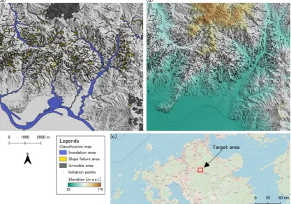
To validate the proposed simulation scheme, we applied it to an actual disaster event that happened on Northern Kyushu Island, Japan in 2017. An area spanning 9 and 8km in the east-west and north-south directions, respectively, around the Akatani River catchment area was selected as the target region. We used the following method to convert the polygonal Geospatial Information Authority of Japan flow traces into a point data set of debris-flow initiation. We defined the debris-debris-flow initiation point in each debris debris-flow trace as the highest point. As most of the debris-flow traces joined each other, we assumed that the highest-elevation cells were the high points within a specific diameter and for the debris-flow trace. The resulting initiation points and the elevation data for the simulation are shown in Fig. 1 (b), which also shows the trace of the flood. The simulation was conducted under the assumptions that all areas were completely saturated, that the erodible soil depth was equally distributed at 1 m, and that all debris flows initiate simultaneously upon commencement of the simulation (T=0 [s]). Other parameters used in the simulation were 𝜌 1.0,𝐶∗
Figure 1: (a) Classification map of damage produced by the 2017 Northern Kyushu Heavy Rainfall Disaster. Source: Geospatial Information Authority of Japan. (b) 5m-resolution elevations and initiation points in the target area for input into reproductive
simulation. (c) Location of target area.
3.2
Calculation
results
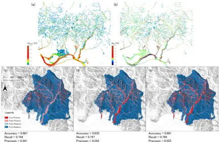
The maximum water level and the terrain deformation (i.e., erosion/deposition) are the critical variables for representing damage caused by the inundation of sediment-laden flood. In this study, these factors were determined by the relative elevations of the water level and ground surface from the initial ground surface, respectively. The maximum water level during the simulation and the final terrain deformation are shown in Fig. 2 (a). A rough comparison reveals that the distribution of each variable agrees with the trace of the disaster shown in Fig. 1 (a).
a predictive map, three thresholdings using the maximum water level and terrain surface deformation were used to produce flooded, landslide, and damaged areas. The landslide area was first compared to the area in which the simulated absolute value of terrain deformation was greater than the threshold value of 0.01 m, as shown in Fig. 2 (c). The comparison produced a high recall value (= 0.744), indicating that the simulated and actual landslide areas mostly coincided. The flooded area was then compared with the area in which the simulated maximum water level was greater than the threshold value (0.01 m), as shown in Fig. 2 (d). This result also produced a high recall value (= 0.747), indicating that the simulated high water-level and inundated areas mostly coincided. Finally, the damaged area itself was determined by comparing the combined flood and landslide area with the area in which the absolute value of 𝑑 was greater than 0𝑚, as this should correspond to locations in which water was present at least once (Fig. 2 (e)). The results had high recall, accuracy, and precision values (0.794, 0.881, and 0.553, respectively), indicating a high degree of coincidence between actual results and prediction. These comparison results allowed us to conclude that the proposed simulation method has a reproductivity suitable for disaster prediction work.
Figure 2: Calculated reproductive simulation results for (a) maximum water level and
(b) terrain surface deformation. (c), (d) and (e) show binary classification results for the quantitative evaluation of simulated results for flooded, landslide and both (water-covered)
area, respectively. Accuracy , recall, and precision are calculated as
4
PREDICTIVE
SIMULATION
EMPLOYING
STATISTICAL
LANDSLIDE
PREDICTION
Deterministic prediction of slope failure location is difficult using current techniques because underground physical parameter conditions are unobservable and unpredictable and there are no robust techniques for the simulation of complex actual topographies. However, watershed topography in mountainous regions has a “concave” characteristic in which all streams converge downstream. In other words, unless the debris flow occurs within different channels in a single Strahler stream order, a given scale of terrain deformation or water level might be reproducible at two or larger orders. If so, the error in predicted location might not strongly affect the downstream area damage. This suggests the possibility of a deterministic, statistically based approach to slope failure prediction. In this section, we describe a statistical landslide prediction model based on logistic regression and use the model to generate artificial landslide datasets. The generated landslide data were applied as input data to a predictive simulation to quantify landslide location uncertainty.
4.1
Statistical
landslide
prediction
model
for
generation
of
artificial
landslide
dataset
Debris flow initiation points, i.e., slope failures or landslides, are essential inputs to the proposed simulation approach. Note that a fully predictive simulation requires data sourced solely from pre-disaster information.
Approaches to generating landslide susceptibility maps include geomorphological mapping, analysis of landslide inventories, heuristic or index-based approaches, process-based
(physically-based) methods, and statistically based modeling (Reichenbach et al., 2018). Of these, physically and statistically based modeling are preferred for quantitative evaluation (Reichenbach et al., 2018). Among the physically based models, which have advantages in terms of physical validity, the infinite slope stability model is a simplified, widely used approach (An et al., 2016; Raia et al., 2014). Although obtaining reliable results requires accurately modeling complicated, heterogeneous underground structures based on field observation or parameter fitting using landslide records, it is not always necessary to use difficult-to-obtain physical parameters in statistically based approaches, and as long as reliable landslide records are used to obtain the statistical relationships, no abnormal results should be produced.
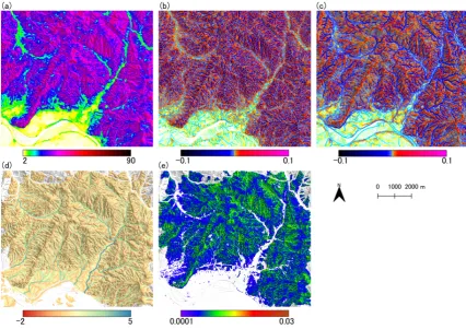
We therefore used a logistic regression model—a preferred approach in statistical modeling—to derive the initiation point likelihood at each top point in the debris-flow trace. The input variables for this model are shown in Figs. 3 (a)–(e). To improve prediction quality, several variables are generally selected as explanatory variables, including curvature, slope, aspect, accumulation, elevation, lithology, precipitation, etc. However, the relationship between landslide occurrence and aspect or elevation is location-dependent and, to ensure generality, we used only four variables: slope, accumulation, and profile/tangential curvature. The predicted probabilities at a 10-m resolution are shown in Fig. 3 (f).
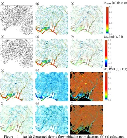
landslide maps. To do this, we generated pseudorandom numbers between zero and one for all meshes in the target areas. For results smaller than the corresponding cell probabilities, the mesh was selected as a debris-flow initiation point. By changing the random-seed generator, 60 sets of debris-flow initiation points were created; these are partially shown in Figs. 4 (a) and (d).
Figure 3: Input (a–d) and output (e) variables of logistic regression: (a) terrain slope (deg); (b) tangential and (c) profile curvature;(d) common logarithm of accumulation area
[m ]; (e) by-point regression-obtained probability of debris-flow initiation. (a) to (d) are calculated using 10-m-resolution DEM. Each value is the average of all neighbors within a
Figure 4: (a) (d) Generated debris-flow initiation point datasets; (b) (e) calculated maximum water level results (T = 3,600[s]); (c) (f) calculated terrain deformation results
(T=3,600[s]). Only first to second cases are shown. (g), (h), and (i) show, respectively, average value, standard deviation, and relative standard deviation for maximum water level.
4.2
Multi
‐
case
predictive
simulation
for
predictive
simulation
using
artificial
landslide
datasets
Sixty simulation cases were conducted using the artificial debris-flow initiation points as input data. Other than the initiation points, all conditions and parameters were held constant across the simulations. Some of the obtained maximum water levels and terrain deformations are shown in Figs. 4 (b), (c), (e), and (f). Roughly similar values of maximum water level and terrain deformation occur in the downstream area, suggesting that the downstream area damage is not sensitive to the landslide initiation point distribution. By contrast, there is high variability in the upstream area closer to the debris-flow initiation points. The variability among the 60 results was quantified using the averaged value (AVE) and standard deviation (SD); relative standard deviation (RSD; =SD/|AVE|)) values were calculated for maximum water level and terrain deformation (Figs. 4 (g)–(l)).
Figs. 4 (g), (h), and (i) show the AVE, SD, and RSD for the maximum water level, respectively. At the outlet of the debris-flow prone basins, the values of AVE range from 0.5–1.0 m; at the bottom of the valley in the downstream area, the value is 1.0–3.0 m, indicating a general increase as the streams flow downstream. By contrast, there are only modest variations in SD of between 0.0–0.2 m. Thus, the RSD values are larger in the upstream space and smaller downstream. As the ratio of the standard deviation and averaged value to the predicted value of the water level, these RSD values indicate the prediction uncertainty owing to landslide location and the predictability of the maximum water level when parameters/conditions other than landslide location are appropriately provided. These results suggest a water-level “predictability” areas located in the valley bottom or downstream alluvial fan that decreases upstream. By contrast, the areas around the outlets of small debris-flow-prone streams have RSDs of approximately 0.5–1.0, indicating a higher degree of predicted-damage uncertainty. Overall, the required precision of landslide location for debris-flow damage prediction differs by location.
The SD, AVE, and RSD values for terrain deformation are shown in Figs. 4 (j), (k), and (l), respectively. Each index follows a trend similar to the corresponding maximum water level index, although the RSD value in the residential area at the bottom of the valley is slightly larger than that for maximum water level.
5
Conclusions
areas.
Our results suggest the following: The damage produced by debris-flow- or sediment-laden floods in the downstream regions of watershed-like topographies is predictable under certain conditions regardless of the location of the sediment sources (slope failures). The dominant factors in terms of predictability are the presence of a catchment-like concave topography, sufficient water to develop a debris flow, and sufficient density of slope failure to join multiple debris flows. Thus, for concave topographies, it is possible to predictively simulate damage resulting when high rainfall yields multiple slope failures and debris flows.
The proposed method relies on several assumptions: • All debris flows initiate simultaneously. • All soils are completely saturated.
• Erodible soil depth is limited to 1m in all regions. • The debris flow material has homogeneous grains.
• Only water in the soil layer, and not additional rainfall, is considered.
Further studies will be required to estimate how each assumption affects the simulation results. However, this study demonstrated the effectiveness of using HPC-based multi-case simulation to evaluate the effects of debris-flow initiation location. A similar approach involving changing each parameter or condition will be used in a future study to quantitatively evaluate each assumption.
6
Acknowledgments
This work was supported by JSPS KAKENHI Grant Number 19K15105 and FOCUS Establishing Supercomputing Center of Excellence (COE). The data that support the findings of this study are available from Geospatial Information Authority of Japan. Restrictions apply to the availability of these data, which were used under license for this study. Data are
available https://www.gsi.go.jp/kiban/ and
https://www.gsi.go.jp/BOUSAI/H29hukuoka_ooita‐heavyrain.html with the permission of
Geospatial Information Authority of Japan.
References
An, H., Viet, T. T., Lee, G., Kim, Y., Kim, M., Noh, S., Noh, J., 2016. Development of time-variant landslide-prediction software considering threedimensional subsurface unsaturated flow. Environmental Modelling and Software 85, 172–183.
Bao, Y., Chen, J., Sun, X., Han, X., Li, Y., Zhang, Y., Gu, F., Wang, J., 2019. Debris flow prediction and prevention in reservoir area based on finite volume type shallow-water model: a case study of pumped-storage hydroelectric power station site in Yi County, Hebei, China. Environmental Earth Sciences 78 (19), 577.
Chen, H. X., Zhang, L. M., Gao, L., Yuan, Q., Lu, T., Xiang, B., Zhuang, W. L., 2017. Simulation of interactions among multiple debris flows. Landslides 14 (2), 595– 615.
Gao, L., Zhang, L. M., Chen, H. X., Shen, P., 2016. Simulating debris flow mobility in urban settings. Engineering Geology.
Geospatial Information Authority of Japan, Digital Map (Basic Geospatial Information), https://www.gsi.go.jp/kiban/
Geospatial Information Authority of Japan, 2017, Information related to the Northern Kyushu heavy rainfall disaster in July 2017,
https://www.gsi.go.jp/BOUSAI/H29hukuoka_ooita-heavyrain.html
Han, X., Chen, J., Xu, P., Niu, C., Zhan, J., 2018. Runout analysis of a potential debris flow in the Dongwopu gully based on a well-balanced numerical model over complex topography. Bulletin of Engineering Geology and the Environment 77 (2), 679–689. Hungr, O., Evans, S. G., Bovis, M. J., Hutchinson, J. N., 2001. A review of the
classification of landslides of the flow type. Environmental and Engineering Geoscience 7 (3), 221–238.
Hungr, O., McDougall, S., 2009. Two numerical models for landslide dynamic analysis. Computers and Geosciences 35 (5), 978–992.
Melo, R., Van Asch, T., Zêzere, J. L., 2018. Debris flow run-out simulation and analysis using a dynamic model. Natural Hazards and Earth System Sciences 18 (2), 555– 570.
Naef, D., Rickenmann, D., Rutschmann, P., W McArdell, B., 2006. Comparison of flow resistance relations for debris flows using a one-dimensional finite element simulation model. Natural Hazards and Earth System Sciences 6 (1), 155–165. Nakatani, K., Hayami, S., Satofuka, Y., Mizuyama, T., 2016. Case study of debris flow
disaster scenario caused by torrential rain on Kiyomizudera, Kyoto, Japan - using Hyper KANAKO system. Journal of Mountain Science 13 (2), 193–202.
O’Brien, J. S., Julien, P. Y., Fullerton, W. T., 1993. TwoDimensional Water Flood and Mudflow Simulation. Journal of Hydraulic Engineering 119 (2), 244–261. Raia, S., Alvioli, M., Rossi, M., Baum, R. L., Godt, J. W., Guzzetti, F., 2014. Improving
predictive power of physically based rainfall-induced shallow landslide models: A probabilistic approach. Geoscientific Model Development 7 (2), 495–514.
Reichenbach, P., Rossi, M., Malamud, B. D., Mihir, M., Guzzetti, F., 2018. A review of statistically-based landslide susceptibility models. Earth-Science Reviews 180 (November 2017), 60–91.
Revellino, P., Hungr, O., Guadagno, F. M., Evans, S. G., 2004. Velocity and runout
simulation of destructive debris flows and debris avalanches in pyroclastic deposits, Campania region, Italy. Environmental Geology 45 (3), 295–311.
Rickenmann, D., Laigle, D., McArdell, B. W., Hu¨bl, J., 2006. Comparison of 2D debris-flow simulation models with field events. Computational Geosciences 10 (2), 241– 264.
Rodríguez-Morata, C., Villacorta, S., Stoffel, M., Ballesteros-C´anovas, J. A., 2019.
Assessing strategies to mitigate debris-flow risk in Abancay province, south-central Peruvian Andes. Geomorphology 342, 127–139.
Natural Hazards and Earth System Sciences 15 (7), 1483–1492. Takahashi, T., 2007. Debris Flow. Taylor & Francis.
Takahashi, T., Nakagawa, H., 1991. Prediction of stony debris flow induced by severe rainfall. Journal of the Japan Society of Erosion Control Engineering 44, 12–19. van Asch, T. W., Tang, C., Alkema, D., Zhu, J., Zhou, W., 2014. An integrated model to
assess critical rainfall thresholds for run-out distances of debris flows. Natural Hazards 70 (1), 299–311.