Sidelobe-Level Suppression for Circular Antenna Array via New
Hybrid Optimization Algorithm Based on Antlion and
Grasshopper Optimization Algorithms
Anas A. Amaireh1, *, Asem S. Al-Zoubi1, and Nihad I. Dib2
Abstract—The suppression of the side-lobe level (SLL) of antenna arrays is a significant factor that can enhance the reliability and validity of a communication system. Recently, metaheuristic algorithms have been widely implemented in the design of antenna arrays, in order to find the optimal minimization for the side-lobe level of the array’s radiation pattern. In this paper, we propose a new hybrid algorithm that combines the characteristics of two stochastic algorithms, Antlion Optimization (ALO) algorithm and Grasshopper Optimization Algorithm (GOA). ALO, which is an evolutionary algorithm, is robust in exploitation and has been effectively used in many articles in the literature. GOA has strong capability of exploration all over the search space due to the swarm nature of the algorithm, which has been proven in several articles in the literature. Therefore, combining these characteristics and overcoming the drawbacks of ALO and GOA are the main motivation behind hybridizing ALO and GOA in one hybrid algorithm. Simulation results show that the proposed hybrid algorithm has a good performance in the radiation pattern optimization of circular antenna array (CAA) and fast convergence rate compared with other strong optimization algorithms, which prove the efficiency, robustness, and stability of the hybrid algorithm.
1. INTRODUCTION
Optimization is the process of finding the global (best) solution(s) for an optimization problem [1]. Among metaheuristic (stochastic) optimization algorithms, which depend on randomness as the main characteristic [2], nature-inspired techniques have been widely used in the literature. Nature-inspired algorithms represent natural actions of creatures, like hunting or flying, which mimic natural problems-solving methods. The following are some of the well-known nature-inspired algorithms and their applications: Particle Swarm Optimization (PSO) [3, 4], Genetic Algorithm (GA) [5, 6], Grey Wolf Optimizer (GWO) [7], Antlion Optimization Technique [8, 9], Galaxy-based Search Algorithm (GbSA) [10], Ant Colony Optimization (ACO) [11], Grasshopper Optimization Algorithm [12, 13], and Hybrid Particle Swallow Swarm Optimization (HPSSO) [14].
Depending on No Free Lunch (NFL) theorem, there is no optimization technique that could solve all optimization problems [15]. This theorem gives the chance to propose new optimization techniques, improve the characteristics of the current methods or combine optimization algorithms together, in order to get more robust and superior methods, which can deal with various problems difficulty and complexity [16].
Using the characteristics of several algorithms when solving optimization problems is the main motivation behind hybridization [17]. Hybridization should combine different types of algorithms, like: population-based metaheuristic algorithms (P-metaheuristics) and single solution metaheuristic
Received 9 April 2019, Accepted 22 May 2019, Scheduled 4 June 2019
* Corresponding author: Anas Atef Amaireh ([email protected]).
algorithms (S-metaheuristics), or swarm metaheuristic algorithms and evolutionary algorithms, to guarantee integration in the new proposed method. So, we choose Antlion optimization technique (ALO) [8] and Grasshopper optimization algorithm (GOA) [13] in this paper, because of the advantages of ALO as an evolutionary algorithm in exploiting the global optimal solution along with balanced exploration of the search space, and the swarm effect of GOA in which the simple search agents of the swarm, with limited capabilities on their own, spread out all over the search space to ensure that all regions are equally explored. Moreover, both methods have been applied successfully in different applications in the literature [9, 12, 18–20], which is another motivation to effectively combine these methods on order to get new robust hybrid method.
Our proposed hybrid algorithm combines the characteristics of these two algorithms; the ability of antlions to hunt other insects in incognito way that lets preys to be consumed in their massive jaws, which shows that ALO is robust in exploitation, and the social relation in the swarm of grasshoppers that swap between the attraction and repulsion forces until reaching a comfortable zone which represents the strong capability of exploration all over the search space [8, 13]. On the other hand, ALO has some drawbacks such as reliance on roulette wheel selection method and elitism, and GOA has other drawbacks which can be represented in exploiting the search space [21]. Moreover, both methods have weakness when they deal with large number of dimensions as mentioned in the results in Section 2.6. Therefore, we do this hybridization to accumulate the complementary characteristics and overcome the drawbacks of ALO and GOA.
Recently, circular antenna arrays (CAA) have been widely investigated in the literature [4, 6, 22, 23]. CAA is a desirable choice, since the main lobe can be directed and focused in any direction in the whole space through 360◦. This array has been used in several fields including radars, navigation systems, and satellite communication [24, 25].
The array elements field must be added constructively in the desired directions and destructively to the other directions, in order to reduce the interference in the side lobes and place nulls in the antenna patterns [19, 22]. Therefore, several optimization algorithms have been used to minimize the side-lobe level in the synthesis of nonuniform CAA, such as Particle Swarm Optimization (PSO) [4, 22, 23, 26], Genetic Algorithm (GA) [6, 22, 26, 27], Dragonfly Algorithm (DA) [28], Seeker Optimization Algorithm (SOA) [24], Non-dominated Sorting Genetic Algorithm II (NSGA-II) [29, 30], Differential evolution [26, 31], Differential Evolution for Multiobjective Optimization (DEMO) [30, 32], and Elitist-Mutated Multi-Objective Particle Swarm Optimization (EM-MOPSO) [30].
Several parameters have to be determined to synthesize circular antenna arrays: feeding currents and their phases, number of elements in the array, position for each element along the circle, and the circle’s radius [33].
The rest of the paper is organized as follows. The proposed hybrid algorithm is discussed and explained in Section 2. The geometry of circular antenna array and the fitness function are detailed in Section 3. Results and discussion are mentioned in Section 4. Finally, the conclusions of the paper are mentioned in Section 5.
2. THE PROPOSED HYBRID ALGORITHM
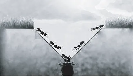
ALO mimics the hunting behavior between antlions and insects inside a cone-shaped trap as shown in Figure 1. GOA simulates the predisposition of Grasshoppers to seek the food resources for solving optimization problems. Consequently, GOA studies the social interactions between adjacent grasshoppers and decides the next position of the grasshopper depending on these interactions.
In this paper, the general idea of the proposed hybrid algorithm assumes that grasshoppers walk randomly on the land and interact with each other by social forces. Then, when they fall in antlions’ traps, the antlions will catch and hunt them as their preys, and finally, consume their body.
The main ideas of the proposed hybrid algorithm are summarized as follows:
- Inside the search space, N grasshoppers will move randomly in random walks, andN antlions will be allowed to catch and hunt them.
- The movement of grasshoppers inside the search space depends essentially on the following factors: a- The social interactions between grasshoppers; switching between attraction and repulsion
Figure 1. Cone-shaped traps and hunting behavior of antlions.
b- The roulette wheel selection method; antlion with more fitness will have more capability to catch grasshoppers.
c- The effect of the elite (most fitness antlion) affects all the grasshoppers’ movements during iterations.
- Once the prey is inside the pit, the antlions shoot sands outside.
- The final step of hunting occurs when the antlion pulls the grasshopper inside the sand and consumes its body.
This section is divided into 6 subsections. The first 3 subsections describe the details and theory of the proposed hybrid algorithm. Subsection 4 defines the advantages of the algorithm. Subsection 5 shows the algorithmic form of our proposed hybrid method, and Subsection 6 illustrates the results of benchmark functions.
2.1. Grasshoppers’ Movement
According to the assumption in our proposed algorithm, grasshoppers that have social interactions among each other will be allowed to move randomly in random walks inside the search space. At the same time, the same number of antlions will be allowed to catch them. These random walks are affected by several critical factors; the roulette wheel selection method, the elite antlion, and antlions’ traps.
Roulette wheel selection method is a mechanism that gives much interest for highly fit search agents, at the expense of less fitness ones. Therefore, the interest in fitter search agents will enhance the exploitation process. On the other hand, not ignoring the less fitness search agents will keep the exploration process alive, because these search agents will have the chance to discover more promised regions.
Elitism represents the idea of letting search agents seek around the promised optima. So, the elite is the antlion that has the best fitness among all other antlions, and it is a good way to save the best solution in each iteration. The elite will be able to affect the movement of all grasshoppers during the iterations [8].
The following equation represents the random walk [8]:
x(t) = [0,cumsum(2r(t1)−1),cumsum(2r(t2)−1), ..., cumsum(2r(tn)−1)] (1)
where cumsum, n, t, and r(t) represent the cumulative sum, the maximum number of iterations, the number of iterations, and the stochastic function, respectively. r(t) is defined as follows [8]:
r(t) =
1 if rand >0.5
0 if rand ≤0.5 (2)
where rand is a random number generated in the interval [0, 1].
In order to keep the random walks inside the search space for all dimensions, the following equation is used for normalization [8]:
Xit=
Xit−ai
×di−Cit
(dti−ai)
where ai and di denote the minimum and maximum of random walk of the ith variable, respectively;
Ct
i represents the minimum; and dti is the maximum of the ith variable at the tth iteration [8].
In our proposed algorithm, we assume that the random walks of grasshoppers are affected by antlions’ traps, similar to the assumption in ALO algorithm. This assumption is mathematically modeled as follows [8]:
cti = Antliontj+ct (4)
dti = Antliontj+dt (5)
where, respectively, ct and dt are the minimum and maximum of all variables at the tth iteration; cti
indicates the minimum of all variables for theith grasshopper; Antliontj is the position of thejth antlion at the tth iteration; and the maximum value of all variables for the ith grasshopper is represented by
dt i [8].
It has been assumed that the random walks’ radius around the antlion decreases proportional to iteration numbers. The following equations represent this [8]:
ct = C
t
I (6)
dt = d
t
I (7)
where ct and dt indicate the minimum and maximum of all variables at the tth iteration, respectively, and I represents a ratio, such thatI = 10w tT wheretrepresents the current iteration, T the maximum number of iterations, and wa constant that depends on the current iteration to define its value (w= 2 when t >0.1T, w= 3 when t >0.5T,w= 4 when t >0.75T, w= 5 when t >0.9T, and w= 6 when
t > 0.95T) [8]. These values increase the value of parameter I in Equations (6) and (7) with respect to the number of iterations. Hence, the decrement ofct and dt will gradually decrease the bounds and allowed region of the search space for the random walks, which rises the exploitation process.
One of the advantages of using random walks and random movement for each search agent is enhancing the exploration process, since randomness increases the capability of discovering more promised regions, randomly, in the search space. On the other hand, the beginning bias of the search by the outstanding search agents may cause loss of diversity and early convergence. Moreover, when all search agents have the same fit, this method does not have enough pressure to select the fittest search agents [21]. This is a drawback for ALO in some optimization problems.
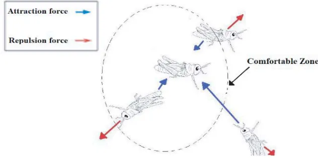
According to Figure 2, a state of interchange between repulsion and attraction occurs between grasshoppers depending on the distance, until reaching a comfortable zone, where neither attraction nor repulsion occurs. The attraction between grasshoppers represents the exploitation process, while the exploration of the search agents inside the search space is represented by the repulsion forces.
The social forces through which the grasshoppers interact with each other are calculated as follows [13]:
s(r) =f e−lr −e−r (8)
where f is the intensity of attraction, and l indicates the attractive length scale. l= 1.5 and f = 0.5 have been chosen in this work. Equation (9), beside its utilization in GOA algorithm, is utilized in the proposed algorithm to reach the comfortable zone slowly, which enhances the opportunity for our hybrid method to explore and exploit the search space around a solution [13].
Xid=c
⎛ ⎜ ⎜ ⎝
N
j=1 j=i
cubd−lbd
2 s X
d j −Xid
X
j−Xi
dij ⎞ ⎟ ⎟
⎠ (9)
whereubdand lbdrepresent the upper and lower bounds in thedth dimension, respectively, ands(r) is
defined in Equation (8).
Parametercrepresents a coefficient that shrinks the three zones in Figure 2; comfort zone, repulsion zone, and attraction zone. So, parameterc is calculated as follows [13]:
c=cmax−lcmax−cmin
L (10)
where cmax and cmin represent the maximum and minimum values, respectively; L indicates the maximum number of iterations; and l is the current iteration [13]. In this work, 1 and 0.00001 have been chosen for cmax and cmin, respectively.
According to Equation (9), the outercis responsible for decreasing the movement of search agents around the optimal values in the promised regions, and the inner c is responsible for decreasing the searching regions around optimal values. This parameter decreases proportional to the number of iterations. So, parameter c controls the exploration at the beginning of iterations with large value of
c, while small value of c will decrease the movement of search agents and shrink the search region of them; in other words, exploiting the search space for global optima.
The previous theory of parameter c already exists in GOA algorithm. But according to the idea of c parameter, it can be concluded that the exploration process takes almost all the iterations, while exploitation does not have enough iterations to find the global optima. This is a drawback for GOA, since the exploration process takes more interest than exploitation, and half of the iterations are more than enough for the algorithm to discover the promised regions in the whole search space. Therefore, in the proposed hybrid algorithm, more interest has been given to exploitation process, in which the hybrid algorithm needs half number of what GOA needs of iterations to reach the same level of exploitation. So, this change balances the exploration and exploitation processes more and gives the algorithm enough iterations to exploit the global optima after the determination of the promised regions in the exploration process. Because of this, Equation (10) has been modified as follows:
ifl≤L/2
c=cmax−lcmaxL−cmin
2
(11)
ifl > L2
c= (L−l+ 1)×
cmin
L×10l
(12)
The modifications in Equations (11) and (12) have been done to increase the decrement of parameter
c proportional to the number of iterations, which leads to more ability to exploit the global optima in the search space.
2.2. Hunting the Prey and Reconstruction of the Pit (Final Step of the Process)
than its following antlion [8]. Consequently, the corresponding antlion will update its position to the position of the consumed grasshopper, which improves its chance to hunt and catch again. The following equation represents this [8]:
Antliontj = Grasshopperti if fGrasshopperti> fAntliontj (13)
where t is the current iteration; Antliontj is the position of selected jth antlion at the tth iteration; Grasshopperti represents the position of the ith grasshopper at the tth iteration; f(Grasshopperti) represents the fitness of the position value for theith grasshopper at thetth iteration; andf(Antliontj) is the fitness value of the position of thejth antlion at thetth iteration [8].
2.3. Next Position Criteria
Three essential factors affect the random walks for each grasshopper around a selected antlion; roulette wheel selection method, the social forces between grasshoppers and the elite. To guarantee the diversity in the proposed hybrid method, the effect of each factor has been calculated and taken into consideration to choose the next position (values of the dimensions). All the values of next positions generated using different factors have been combined in one matrix and ranked depending on their fitness. Then, three samples of this matrix have been chosen; a most fitness, an average fitness, and a least fitness samples, such that the number of chosen sampled values is the same as search agents’ number. Choosing a low fitness sample will give the opportunity to other regions in the search space to be scanned, which improves the exploration process in this algorithm. At the same time, choosing high fitness sample will enhance the exploitation in this proposed algorithm. Thus, better diversity of search agents is provided with this combination of exploration and exploitations.
2.4. Hybrid Algorithm Advantage
The advantages of our proposed hybrid method can be summarized in its ability to explore the search space, due to the combination of several factors; the population nature of the proposed algorithm that reduces local optima stagnation, the repulsion force in grasshopper’s social interactions, the random walks of grasshoppers that let them walk randomly in the search space, and choosing different samples of average and less fitness search agents from next position’s matrix, which gives the chance to scan and explore other promised regions than the one with local optima.
Further, the proposed hybrid algorithm improves the characteristic of exploitation of the global optima because of the following reasons: the attraction forces of social interactions between grasshoppers, parametercmodification that improves the balance between exploration and exploitation, roulette wheel selection method which gives more interest for fitter search agents, and parameter w in Equations (6) and (7), which shrinks the searched region depending on the number of iterations.
The benefits of hybridization can be concluded in overcoming the drawbacks of ALO and GOA. Roulette wheel method in selecting the next positions is the main disadvantage of ALO, which may cause, as mentioned previously, early convergence, loss of diversity, and no enough pressure to select the fittest search agents when they have the same fit. On the other hand, parametercis the main drawback for GOA algorithm, which does not give enough iterations for the exploitation process.
Therefore, the combination of all previous factors significantly improves the exploration and exploitation process in our proposed hybrid algorithm. This increases the diversity of the search agents in the search space and leads to high probability for local optima stagnation avoidance.
Furthermore, the intensity of search agents in the proposed algorithm has been decreased rapidly compared with ALO and GOA, due to the modification of parameterc and its combination with other shrinking factors like w. Therefore, compared to ALO and GOA, the hybrid algorithm guarantees fast and mature convergence.
2.5. Algorithmic Form of the Proposed Hybrid Technique
parameter for searching area. l: Current iteration number. cmax: Maximum value in equation 10. cmin: Minimum value in equation 10. f: The intensity of attraction. l: The attractive length scale. w: Constant adjusts the accuracy of exploitation. Xd
i: The position of ith iteration and dth dimension. L: Maximum number of iterations.
Output: Best grasshopper positions and its fitness value.
Algorithm:
Initialize the input parameters
Initialize the first population of grasshopper swarm and antlions randomly
while the end criterion is not satisfied
Update c using Equation (11) and Equation (12) for every grasshopper
Normalize the distances between grasshoppers
Update the position of the current search agent by the Equation (9) Select an antlion using Roulette wheel
Update c and d using equations, Equations (6) and (7)
Create a random walk and normalize it using Equation (1) and (3)
Gather the positions of grasshoppers that affected by roulette wheel, elite and social forces in one matrix Choose 3 different samples with different fitness
Update the position of the grasshoppers end for
Bring the current search agent back if it goes outside the boundaries Calculate the fitness of all grasshoppers
Replace an antlion with its corresponding grasshopper it if becomes fitter (Equation (13))
Update elite if an antlion becomes fitter than the elite Update the positions of the grasshoppers randomly end while
Return elite
2.6. Results of Benchmark Mathematical Function
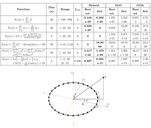
The performance of our proposed algorithm has been tested using three different benchmark functions; unimodal, multimodal, and composite test functions. Table 1 shows six mathematical benchmark functions with a comparison of the results of our proposed hybrid method with ALO and GOA. In [8, 13], ALO and GOA have been compared with other optimization techniques like PSO, SMS, BA, FPA, CS, FA, GA, DE, and Gravitational Search Algorithm (GSA), and it was found that both algorithms were slightly better than all other compared optimization techniques. Dim indicates the dimension of the function; Range is the boundary of the function’s search space; andfminis the optimum value. According
to Table 1, the results prove the superiority of our proposed hybrid algorithm over ALO and GOA in all the mentioned benchmark functions. Moreover, the proposed method reaches the exact global optimum in some functions, while ALO and GOA stagnate in local optimum. This proves the ability of our hybrid method to effectively explore and exploit the search space. The results show the great advantages of our hybrid algorithm in overcoming the drawbacks of ALO and GOA.
3. GEOMETRY AND FITNESS FUNCTION
Table 1. Benchmark test functions and their results.
Function Dim
(n) Range fmin
Hybrid ALO GOA
Best sol. Std. Best sol. Std. Best sol. Std.
F1(x) =n
i=1x 2
i 30 [−100, 100] 0
2.448 e-39 6.300 e-40 1.455 e-07 1.352 e-06 0.057 3 0.75 0
F2(x) = n
i=1|xi|+ n
i=1|xi| 30 [−10, 10] 0
3.388
e-20 0 0.919
52.69 6 0.150 2 21.9 28
F3(x) = 0.5 +sin2√x21+x22−0.5
1+0.01(x2
1+x22)2 2 [−10, 10] 0 0 0
1.554 e-15 2.971 e-14 7.216 e-15 1.47 e-14
F4(x) =n
i=1[x 2
i−10 cos(2πxi) + 10] 30 [−5.12, 5.12] 0 0 16.85
69 33.82 8 19.54 6 35.83 4 24.3 29
F5(x) =D
i=1x2i + (Di=10.5ixi)2
+(D
i=10.5ixi)4
30 [−10, 10] 0 4.317
e-40
1.478 e-38
1.311 e + 02
1.305 e + 02
46.17 6
58.8 86
F6(x) =x2
2−4π5.12x21+π5x1
+101− 1 8π
cos(x1) + 10 2
[−5, 10]
[0, 15] 0.398 0.397
9.085 e-15 0.397 1.887 e-14 0.397 1.40 e-13
Figure 3. Geometry of a non-uniform circular antenna array withN isotropic antennas.
The radiation pattern for such a geometry can be described by the following array factor equation [25]:
AF(θ, ϕ) =
N
n=1
Inexp (j[kasin(θ) cos (ϕ−ϕn) +αn]) (14)
where
ka = 2π
λ a=
N
i=1
di (15)
ϕn =
2π n i=1 di ka (16)
To focus the main beam in (θo, ϕo) direction, the excitation phase is assumed as follows [25]:
In and ϕn represent the excitation amplitude and the angular position of the nth element in the x-y
plane, respectively. dn represents the arc distance between two adjacent elements (in terms of λ). θ
represents the elevation angle which is measured from the positive z-axis. θ is assumed to equal 90◦, since the array factor in the x-y plane will be of interest. ϕ is the azimuth angle measured from the positive x-axis. Furthermore, θo and ϕo show the direction of the main lobe. For simplicity, in all
coming examples, the main lobe is assumed to be directed along the positivex-axis, such thatθo = 90◦
and ϕo= 0◦.
The goal in any antenna array problem is to optimize many key parameters such as side-lobe level, gain, size, and radiation pattern, which can be used to evaluate a specific fitness function. In this paper, the goal is to reduce the maximum side-lobe level for specific first null beam width (FNBW). So, the following shows the used fitness function [33]:
Fitness = 10 log
(W1F1+W2F2)/|AFmax|2
(18)
F1 = |AF(ϕnu1)|2+|AF(ϕnu2)|2 (19)
F2 = max
|AF(ϕms1)|2,|AF(ϕms2)|2
(20)
A desired FNBW can be obtained by minimizing the array factor at two angles ϕnu1 and ϕnu2, where
ϕnu denotes the angle at a null. So, the FNBW =ϕnu2−ϕnu1 = 2ϕnu2 [33].
The range of angles in which the optimization process works to minimize the side-lobe level are represented in two bands; the lower band (from−180◦ toϕnu1) asϕms1 and the upper band (fromϕnu2
to 180◦) as ϕms2. Therefore, functionF2 minimizes the AF in the side-lobe regions around the major
lobe.
AFmaxdenotes the maximum value of the array factor at (θo, ϕo). W1andW2 are weighting factors
which will be chosen in each example respectively. Thus, for the design of CAA with minimum side-lobe level, the optimization problem is to search for the current amplitudes (In’s) and the arc distances
between the elements (dn’s) that minimize the fitness function.
4. RESULTS AND DISCUSSION
All the examples in this paper have been optimized for 20 independent runs, and the one with the least fitness function is shown here. Examples with optimized excitation currents have been normalized with respect to largest current value.
4.1. Example 1: 8, 10, 12-Element CAA
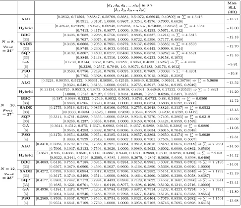
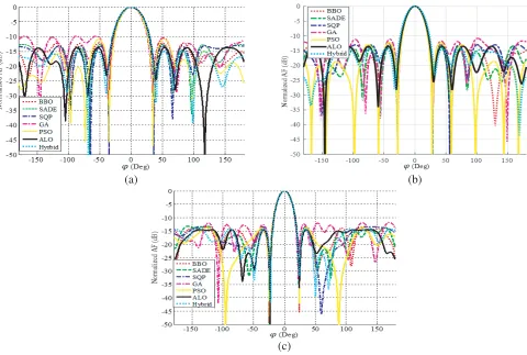
In this example, a circular antenna array with 8, 10, and 12 elements is optimized using ALO and the hybrid method. The obtained results are compared with those obtained using BBO [33], Self-Adaptive DE (SADE) [33], Sequential Quadratic Programming (SQP) [33], GA [6], and PSO [4]. The best values of the maximum side-lobe level for these algorithms are shown in Table 2. The maximum SLL for 8-element case, which is obtained using ALO, the hybrid method, BBO, SADE, SQP, GA, and PSO in (dB) are −13.71, −15.00, −12.18, −12.70, −13.16, −9.81, and −10.8, respectively. It can be noticed that the hybrid algorithm gets better SLL than other algorithms, which proves the ability of the hybrid algorithm to outperform other strong techniques. The maximum SLLs obtained using ALO and the hybrid method in 10-element CAA case are −13.52 dB and −14.20 dB, respectively, while−12.72 dB,
Table 2. Optimum values of current amplitudes and spacing for optimized, 10 and 12-element CAA.
[d1, d2, d3, ..., dN] inλ’s [I1, I2, I3, ..., IN]
Max. SLL (dB)
N= 8, ϕnu2
= 34◦
ALO [0.3832, 0.71592, 0.86847, 0.58769, 0.3681, 0.54072, 0.66945, 0.40809]⇒
= 4.5416
[0.5911, 0.3107, 1.0000, 0.9867, 0.3254, 0.4976, 0.7003, 0.6026] −13.71
Hybrid [0.32632, 0.82689, 0.80623, 0.60948, 0.82323, 0.67637, 0.24608, 0.22379]⇒
= 4.5384
[0.7413, 0.4178, 0.8977, 1.0000, 0.3644, 0.4233, 0.5671, 0.1342] −15.00
BBO
[33] [0.3406, 0.7682, 0.2988, 0.5756, 0.6627, 0.8805, 0.6337, 0.4214]⇒
= 4.5815
[0.7637, 0.6075, 0.1090, 1.0000, 0.8722, 0.5396, 0.7177, 0.4858] −12.18
SADE
[33] [0.3438, 0.6668, 0.2059, 0.7951, 0.6272, 0.8437, 0.8295, 0.3383]⇒
= 4.6503
[0.8749, 0.2302, 0.4633, 0.9542, 1.0000, 0.6442, 0.9099, 0.1844] −12.70
SQP
[33] [0.3192, 0.3867, 0.4809, 0.8277, 0.6450, 0.8066, 0.8573, 0.3287]⇒
= 4.6521
[0.8849, 0.1438, 0.5516, 1.0000, 0.9998, 0.6233, 0.9158, 0.1053] −13.16
GA
[6] [0.1739, 0.3144, 0.662, 0.7425, 0.6297, 0.8969, 0.4633, 0.5267]⇒
= 4.4094
[0.3289, 0.2537, 0.7849, 1.0, 0.9171, 0.5183, 0.6176, 0.4612] −9.81
PSO
[4] [0.3590, 0.5756, 0.2494, 0.7638, 0.6025, 0.8311, 0.7809, 0.3308]⇒
= 4.4931
[0.7765, 0.3928, 0.6069, 0.8446, 1.0000, 0.7015, 0.9321, 0.3583] −10.8
N= 10, ϕnu2
= 27◦
ALO [0.3224, 0.90353, 0.5122, 0.96631, 0.50981, 0.42519, 0.68649, 0.29396, 0.96161, 0.38708]⇒
= 5.9686
[0.9324, 0.5491, 0.6133, 1.0000, 0.9151, 0.2755, 0.3917, 0.6184, 0.9195, 0.8949] −13.52
Hybrid [0.33134, 0.46725, 0.95313, 0.93073, 0.54016, 0.9018, 0.83961, 0.44049, 0.27222, 0.20533]⇒
= 5.8821
[1.0000, 0.2648, 0.7127, 0.9852, 0.9451, 0.6948, 0.2659, 0.6235, 0.6497, 0.4569] −14.20
BBO
[33] [0.387, 0.9088, 0.3232, 0.2549, 0.8932, 0.5083, 0.8781, 0.6733, 0.88, 0.3498]⇒
= 6.0566
[0.8848, 0.5265, 0.3690, 0.3744, 1.0000, 1.0000, 0.6374, 0.5803, 0.8792, 0.5606] −12.72
SADE
[33] [0.2775, 0.9516, 0.5141, 0.9865, 0.6166, 0.9703, 0.2755, 0.2648, 0.8826, 0.3137]⇒
= 6.0532
[00.9333, 0.5834, 0.4528, 1.0000, 0.9620, 0.3544, 0.2959, 0.4202, 0.8792, 0.1412] −13.43
SQP
[33] [0.3311, 0.4761, 0.5888, 0.3355, 1.0000, 0.5818, 0.9346, 0.7570, 0.7405, 0.2865]⇒
= 6.0319
[0.9288, 0.1237, 0.3838, 0.5450, 1.0000, 0.8450, 0.7054, 0.4424, 0.8559, 0.1589] −13.02
GA
[6] [0.3641, 0.4512, 0.275, 1.6373, 0.6902, 0.9415, 0.4657, 0.2898, 0.6456, 0.3282]⇒
= 6.0886
[0.9545, 0.4283, 0.3392, 0.9074, 0.8086, 0.4533, 0.5634, 0.6015, 0.7045, 0.5948] −11.03
PSO
[4] [0.3170, 0.9654, 0.3859, 0.9654, 0.3185, 0.3164, 0.9657, 0.3862, 0.9650, 0.3174]⇒
= 5.9029
[1.0000, 0.7529, 0.7519, 1.0000, 0.5062, 1.0000, 0.7501, 0.7524, 1.0000, 0.5067] −12.31
N= 12, ϕnu2
= 23◦
ALO [0.3410, 0.5083, 0.2792, 0.7175, 0.7388, 0.7921, 0.5084, 0.9812, 0.3618, 0.8489, 0.8675, 0.3209]⇒
= 7.2661 [0.7906, 0.1037, 0.3133, 0.7593, 0.3020, 1.0000, 0.9989, 0.5623, 0.6002, 0.6089, 0.6862, 0.6560] −14.56
Hybrid [0.3571, 0.935, 0.4866, 0.8501, 0.7115, 0.4867, 0.9440, 0.1871, 0.2680, 0.8213, 0.8238, 0.3430]⇒
= 7.2153 [0.9322, 0.3441, 0.7926, 0.3505, 0.8585, 1.0000, 0.3679, 0.2897, 0.5656, 0.6006, 0.6908, 0.6496] −14.12
BBO
[33] [0.4083, 0.6416, 0.7554, 0.7185, 0.6943, 0.3818, 0.3284, 0.8152, 0.9981, 0.3097, 0.7983, 0.3701]⇒
= 7.2196 [0.6567, 0.3879, 0.6960, 0.4596, 0.5627, 0.9600, 0.4168, 0.5890, 0.5368, 0.6230, 0.6910, 1.0000] −14.01
SADE
[33] [0.4272, 0.6798, 0.6380, 0.6954, 0.9017, 0.5223, 0.7686, 0.6235, 0.2582, 0.5151, 0.8151, 0.3343]⇒
= 7.1792 [0.3617, 0.3740, 0.3498, 0.6514, 1.0000, 0.8604, 0.4864, 0.3960, 0.3696, 0.3390, 0.5058, 0.8387] −13.19
SQP
[33] [0.4177, 0.5963, 0.7442, 0.7173, 0.7994, 0.4433, 0.8958, 0.7129, 0.7622, 0.4557, 0.1607, 0.3786]⇒
= 7.0841 [0.4685, 0.4221, 0.6701, 0.3644, 0.6449, 0.8077, 0.4698, 0.4986, 0.5102, 0.1341, 0.2746, 1.0000] −13.41
GA
[6] [0.4936, 0.4184, 1.4474, 0.7577, 0.4204, 0.5784, 0.4520, 0.8872, 0.7514, 0.4202, 0.4223, 0.7234]⇒
= 7.7724 [0.2064, 0.5461, 0.2246, 0.6486, 0.7212, 0.7993, 0.5277, 0.3485, 0.5125, 0.4475, 0.5233, 0.8553] −11.80
PSO
[4] [0.2569, 0.8509, 0.6607, 0.7057, 0.8540, 0.3734, 0.1609, 0.8321, 0.6464, 0.7079, 0.8330, 0.2682]⇒
= 7.1501 [0.9554, 0.6641, 0.7109, 0.7769, 1.0000, 1.0000, 0.3958, 0.7162, 0.6746, 0.7695, 0.9398, 0.6415] −13.68
12-element CAA. Note that the number of search agents of ALO and the hybrid method in 8, 10, and 12-element cases are (50, 50), (50, 50), and (150, 50), respectively. The maximum numbers of iterations are 300 for 8 and 10-element cases, and 500 for 12-element case. Further, the weighting factors of the fitness function (W1 and W2) for 8, 10, and 12-element cases are (1, 5), (1, 10), and (1, 1), respectively.
4.2. Example 2: 20-Element CAA
In this example, 50 search agents, 500 iterations, W1 = 1, and W2 = 5 have been used. Similar to
(a) (b)
(c)
Figure 4. (a) Radiation patterns for the optimized 8-element CAA. (b) Radiation patterns for the optimized 10-element CAA. (c) Radiation patterns for the optimized 12-element CA.
(a) (b) (c)
Figure 5. (a) Convergence curves of ALO and hybrid method for 8-element CA. (b) Convergence curves of ALO and hybrid method for 10-element CAA. (c) Convergence curves of ALO and hybrid method for 12-element CAA.
4.3. Example 3: 20-Element CAA with Constant Circumference
(a) (b) (c)
Figure 6. (a) whisker plot of ALO and hybrid method in 20 runs for 8-element. (b) Box-and-whisker plot of ALO and hybrid method in 20 runs for 10-element. (c) Box-and-Box-and-whisker plot of ALO and hybrid method in 20 runs for 12-element.
(a) (b) (c)
Figure 7. (a) Radiation patterns for the optimized 20-element CA. (b) Convergence curves of ALO and hybrid method. (c) Box-and-whisker plot of ALO and hybrid method in 20 runs.
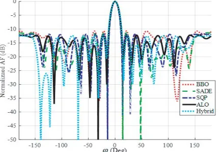
Figure 8. Radiation patterns for the optimized 20-element CAA using fitness function (21).
different optimization techniques fair, the circumference of the optimized arrays must be almost the same as that of the uniform array. In order to accomplish this, the following modified fitness function has been used [33]:
Table 3. Optimum values of current amplitudes and spacing for the optimized N = 20 CAA.
N= 20 ϕnu2= 14◦
[d1, d2, d3, ..., d20] inλ’s [I1, I2, I3, ..., I20]
Max. SLL (dB)
ALO
[0.60943, 0.59257, 0.87452, 0.78683, 0.54473, 0.9433, 0.96702, 0.98326, 0.42234, 0.61703, 0.44987, 0.88652, 0.23454, 0.86473, 0.29602, 0.99958, 0.66856, 0.95044, 0.60746, 0.59609]
⇒= 13.8948
[0.8229, 0.5180, 0.5919, 0.2521, 0.6313, 0.4851, 0.5649, 0.9427, 0.9433, 0.9923, 0.8665, 0.4725, 0.3112, 0.4011, 0.2856, 0.5601, 0.7973, 0.9022, 0.9046, 1.0000]
−14.39
Hybrid
[0.48636, 0.37306, 0.73972, 0.15148, 0.36325, 0.81309, 0.73599, 0.90463, 0.70386, 0.33118, 0.4698, 0.99927, 0.63298, 0.18699, 0.39993, 0.2781, 0.57851, 0.90866, 0.42596, 0.25917]
⇒= 10.7420
[0.7364, 0.4895, 0.2950, 0.8534, 0.3807, 0.3672, 0.5657, 0.5512, 1.0000, 0.9192, 0.4595, 0.4797, 0.4012, 0.4541, 0.2529, 0.4946, 0.6557, 0.7004, 0.6785, 0.8198]
−14.98
BBO
[33]
[0.4196, 0.4588, 1.0000, 0.4406, 0.6314, 0.3635, 0.8939, 0.3215, 1.0000, 0.4786, 0.4856, 0.5848, 0.4761, 0.5695, 0.8245, 0.9013, 0.7483, 0.8833, 0.4748, 0.4417]⇒= 12.3978 [0.8227, 0.9057, 0.3545, 0.1653, 0.7815, 0.6918, 0.6865, 0.7171, 1.0000, 1.0000, 0.9981, 0.7308,
1.0000, 0.6543, 0.9493, 0.1000, 0.5944, 0.6473, 0.5730, 1.0000]
−13.84
SADE
[33]
[0.4825, 0.1795, 0.1793, 0.6164, 0.9753, 0.3628, 0.6046, 0.9890, 0.2913, 0.9223, 0.5750, 0.7937, 0.9161, 0.8519, 0.9921, 0.5791, 0.2997, 0.7233, 0.5166, 0.3347]⇒= 12.1852 [0.9072, 0.4465, 0.1364, 0.7688, 0.6309, 0.5683, 0.5877, 0.2080, 0.3060, 1.0000, 0.9771, 0.5235,
0.7805, 0.3250, 0.7083, 0.6721, 0.6070, 0.8726, 0.6762, 0.8076]
−13.95
SQP
[33]
[0.5682, 0.6833, 0.4381, 0.4709, 0.7318, 0.8736, 0.6329, 0.2492, 0.9944, 0.6006, 0.5653, 1.0000, 0.8636, 0.8893, 0.3727, 0.3865, 0.4148, 0.5996, 0.5457, 0.4453]⇒= 12.3258 [0.8708, 0.2126, 0.6157, 0.5070, 0.2995, 0.4988, 0.3782, 0.3621, 0.8598, 1.0000, 0.6950, 0.5762,
0.7123, 0.3460, 0.1815, 0.6140, 0.3407, 0.3590, 0.8188, 0.9923]
−14.87
Uniform
[0.5, 0.5, 0.5, 0.5, 0.5, 0.5, 0.5, 0.5, 0.5, 0.5, 0.5, 0.5, 0.5, 0.5]
⇒= 10.0
[1.0, 1.0, 1.0, 1.0, 1.0, 1.0, 1.0, 1.0, 1.0, 1.0, 1.0, 1.0, 1.0, 1.0]
−6.08
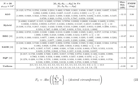
Table 4. Optimum values of current amplitudes and spacing for the optimized 20-element CAA using fitness function (21).
N= 20 ϕnu2= 14◦
[d1, d2, d3, ..., d20] inλ’s [I1, I2, I3, ..., I20]
Max. SLL (dB) FNBW (deg) ALO
[0.1125, 0.7710, 0.3783, 0.8338, 0.2914, 0.4662, 0.7609, 0.3821, 0.8508, 0.5007, 0.3033, 0.6937, 0.5245, 0.2902, 0.6090, 0.2816, 0.6267, 0.4127, 0.4014, 0.5091] =⇒= 10
[1.0000, 0.8468, 0.5623, 0.7603, 0.2219, 0.4930, 0.4620, 0.3592, 0.8579, 0.6492, 0.4555, 0.3381, 0.5437, 0.8799, 0.3620, 0.4762, 0.5176, 0.7947, 0.6556, 0.9128]
−12.15 3.06
Hybrid
[0.43962, 0.68527, 0.1315, 0.18265, 0.57491, 0.70708, 0.93932, 0.28695, 0.84466, 0.34695, 0.13591, 0.33026, 0.50352, 0.99359, 0.37457, 0.41363, 0.96354, 0.51167, 0.32517, 0.30925]⇒= 10 [0.3196, 0.1734, 0.2017, 0.6241, 0.4340, 0.5036, 0.5510, 0.2000, 0.8267, 0.9553, 0.4398, 0.4800, 0.9311,
0.5354, 0.7467, 0.4909, 0.7467, 0.6050, 0.7531, 0.2119, 1.0000]
−12.35 30.4
BBO[33]
[0.3992, 0.9735, 0.2235, 0.3108, 1.0000, 0.2110, 0.4899, 0.1000, 0.3585, 0.4811, 0.2717, 0.5740, 0.7261, 1.0000, 0.3988, 0.2548, 0.8606, 0.5380, 0.5212, 0.3077]⇒= 10
[0.5576, 0.1000, 0.9253, 0.6877, 1.0000, 0.3850, 0.1000, 0.1000, 0.3295, 0.1000, 1.0000, 0.8999, 0.5202, 0.6851, 0.6877, 1.0000, 0.4435, 0.2389, 0.6996, 1.0000]
−10.67 28.6
SADE[33]
[0.2188, 0.2808, 0.7180, 0.3800, 0.8207, 0.2932, 0.9706, 0.6226, 0.5565, 0.1364, 0.4640, 0.5064, 0.8742, 0.1964, 0.8028, 0.2789, 0.4280, 0.6616, 0.4842, 0.3062]⇒= 10
[0.7398, 0.4071, 0.3937, 0.7197, 1.0000, 0.9281, 0.7220, 0.3150, 0.8843, 0.7853, 0.5352, 0.3133, 0.6459, 0.9790, 0.9843, 0.7044, 0.1857, 0.3126, 0.8326, 0.6337]
−11.30 28.9
SQP[33]
[0.1817, 0.1738, 0.8299, 0.7268, 0.2955, 0.8317, 0.7392, 0.8753, 0.2633, 0.1484, 0.2256, 0.9999, 0.7963, 0.3393, 0.3556, 0.4066, 0.9978, 0.5057, 0.2006, 0.1070]⇒= 10
[0.1278, 0.4208, 0.1790, 0.7576, 1.0000, 0.8536, 0.3456, 0.1000, 0.9955, 0.5949, 0.3683, 0.3726, 0.5160, 0.9991, 0.5923, 0.6132, 0.1000, 0.3723, 0.3600, 0.7845]
−11.81 28.22
Uniform [0.5, 0.5, 0.5, 0.5, 0.5, 0.5, 0.5, 0.5, 0.5, 0.5, 0.5, 0.5, 0.5, 0.5]⇒
= 10.0
[1.0, 1.0, 1.0, 1.0, 1.0, 1.0, 1.0, 1.0, 1.0, 1.0, 1.0, 1.0, 1.0, 1.0] −6.08 28
F3 = Abs
N
i=1
di
−(desired circumference)
(22)
and max SLL for a 20-element CAA. In this table, the summation of the spacings between elements for all techniques equals 10λ, which is the same as uniform array. Figure 8 demonstrates the radiation patterns for ALO, the hybrid method, BBO, SADE, and SQP compared with uniform antenna array. It can be concluded that the hybrid algorithm and ALO beat other methods. Here, 180 and 50 search agents have been used for ALO and the hybrid method, respectively. Moreover, the numbers of iterations and weighting factors used for both proposed algorithms are 500,W1 = 1 andW2= 10.
5. CONCLUSION
In this work, we propose a new hybrid algorithm that combines the characteristics of ALO and GOA, by using the advantages of both techniques. The proposed algorithm mathematically implements the random walks of antlions and elitism in addition to the social forces in grasshopper’s swarm. Consequently, both algorithms are utilized in a proper hybridization. Moreover, the new hybrid algorithm and ALO are successfully introduced in the synthesis of circular antenna arrays. In this paper, five cases are discussed; 8-element, 10-element, 12-element, 20-element, and 20-element with constant circumference. The results show that the proposed hybrid algorithm is very competitive in reducing the SLL compared to other methods like ALO, PSO, GA, SADE, SQP, and BBO.
REFERENCES
1. Mirjalili, S., “Moth-flame optimization algorithm: A novel nature-inspired heuristic paradigm,”
Knowledge-based Systems, Vol. 89, 228–249, 2015.
2. Spall, J. C., Introduction to Stochastic Search and Optimization: Estimation, Simulation, and Control, John Wiley & Sons, 2003.
3. Eberhart, R. C. and J. Kennedy, “A new optimizer using particle swarm theory,” Proceedings of the Sixth International Symposium on Micro Machine and Human Science, Nagoya, Japan, 1995. 4. Shihab, M., Y. Najjar, N. Dib, and M. Khodier, “Design of non-uniform circular antenna arrays
using particle swarm optimization,” Journal of Electrical Engineering, Vol. 59, 216–220, 2008. 5. Holland, J. H., “Genetic algorithms,” Scientific American, Vol. 267, 66–72, 1992.
6. Panduro, M., A. Mendez, R. Dominguez, and G. Romero, “Design of non-uniform circular antenna arrays for side lobe reduction using the method of genetic algorithms,” International Journal of Electronics and Communications, Vol. 60, 713–717, 2006.
7. Mirjalili, S., S. M. Mirjalili, and A. Lewis, “Grey wolf optimizer,”Advances in Engineering Software, Vol. 69, 46–61, 2014.
8. Mirjalili, S., “The ant lion optimizer,” Advances in Engineering Software, Vol. 83, 80–98, 2015. 9. Dib, N., A. Amaireh, and A. Al-Zoubi, “On the optimal synthesis of elliptical antenna arrays,”
International Journal of Electronics, Vol. 106, No. 1, 121–133, 2019.
10. Shah-Hosseini, H., “Principal components analysis by the galaxy-based search algorithm: A novel metaheuristic for continuous optimization,” International Journal of Computational Science and Engineering, Vol. 6, 132–140, 2011.
11. Colorni, A., M. Dorigo, and V. Maniezzo, “Distributed optimization by ant colonies,” Proceedings of the First European Conference on Artificial Life, 1991.
12. Amaireh, A., A. Alzoubi, and N. Dib, “Design of linear antenna arrays using antlion and grasshopper optimization algorithms,”IEEE Jordan Conference on Applied Electrical Engineering and Computing Technologies, 2017.
13. Saremi, S., S. Mirjalili, and A. Lewis, “Grasshopper optimisation algorithm: Theory and application,”Advances in Engineering Software, Vol. 105, 30–47, 2017.
14. Kaveh, A., T. Bakhshpoori, and E. Afshari, “An efficient hybrid particle swarm and swallow swarm optimization algorithm,” Computers and Structures, Vol. 143, 40–59, 2014.
16. Blum, C., A. Roli, and M. Sampels, Hybrid Metaheuristics — An Emerging Approach to Optimization, Springer, 2008.
17. Mirjalili, S., G. Wang, and L. S. Coelho, “Binary optimization using hybrid particle swarm optimization and gravitational search algorithm,”Neural Computing &Applications, Vol. 25, 1423– 1435, 2014.
18. Mafarja, M., I. Aljarah, A. Heidari, A. Hammouri, H. Faris, A. Al-Zoubi, and S. Mirjalili, “Evolutionary population dynamics and grasshopper optimization approaches for feature selection problems,” Knowledge-based Systems, Vol. 145, No. 1, 25–45, 2018.
19. Wu, J., H. Wang, N. Li, P. Yao, Y. Huang, Z. Su, and Y. Yu, “Distributed trajectory optimization for multiple solar-powered UAVs target tracking in urban environment by adaptive grasshopper optimization algorithm,” Aerospace Science and Technology, Vol. 70, 497–510, 2017.
20. Heidari, A., H. Faris, I. Aljarah, and S. Mirjalili, “An efficient hybrid multilayer perceptron neural network with grasshopper optimization,”Soft Computing, 1–18, 2018.
21. El-Ghazali, T., Metaheuristics: From Design to Implementation, Wiley & Sons, 2009.
22. Panduro, M. A., C. A. Brizuela, L. I. Balderas, and D. A. Acosta, “A comparison of genetic algorithms, particle swarm optimization and the differential evolution method for the design of scannable circular antenna arrays,” Progress In Electromagnetics Research B, Vol. 13, 171–186, 2009.
23. Mahmoud, K., M. Eladawy, R. Bansal, S. Zainud-Deen, and S. Ibrahem, “Analysis of uniform circular arrays for adaptive beamforming applications using particle swarm optimization algorithm,” International Journal of RF and Microwave Computer-Aided Engineering, Vol. 18, 42–52, 2008.
24. Guneya, K. and S. Basbug, “A parallel implementation of seeker optimization algorithm for designing circular and concentric circular antenna arrays,” Applied Soft Computing, Vol. 22, 287– 296, 2014.
25. Balanis, C., Antenna Theory: Analysis and Design, Wiley, New York, 2012.
26. Panduro, M. A. and C. A. Brizuela, “A comparative analysis of the performance of GA, PSO and DE for circular antenna arrays,”IEEE Antennas and Propagation Society International Symposium, Charleston, USA, 2009.
27. Reyna, A., M. Panduro, D. Covarrubias, and A. Mendez, “Design of steerable concentric rings array for low side lobe level,” Scientia Iranica, Vol. 19, No. 3, 727–732, 2012.
28. Babayigit, B., “Synthesis of concentric circular antenna arrays using dragonfly algorithm,”
International Journal of Electronics, Vol. 105, 784–793, 2017.
29. Panduro, M. and C. Brizuela, “Evolutionary multi-objective design of non-uniform circular phased arrays,” COMPEL International Journal of Computations and Mathematics in Electrical, Vol. 27, No. 2, 551–566, 2008.
30. Panduro, M., C. Brizuela, J. Garza, S. Hinojosa, and A. Maldonado, “A comparison of NSGA-II, DEMO, and EM-MOPSO for the multi-objective design of concentric rings antenna arrays,”
Journal of Electromagnetic Waves and Applications, Vol. 27, No. 9, 1100–1113, 2013.
31. Elizarraras, O., A. Mendez, A. Maldonado, M. Panduro, and D. Covarrubias, “Design of circular array of circular subarrays for scannable pattern using rotational symmetry,” IEEE International Symposium on Antennas and Propagation &USNC/URSI National Radio Science Meeting, 2017. 32. Garza, L., M. Panduro, D. Covarrubias, and A. Maldonado, “Multiobjective synthesis of steerable UWB circular antenna array considering energy patterns,”International Journal of Antennas and Propagation, Vol. 2015, Article ID 789094, 9 pages, 2015.