in GF(3
6n)
Takuya Hayashi1, Naoyuki Shinohara2, Lihua Wang2, Shin’ichiro Matsuo2,
Masaaki Shirase1, and Tsuyoshi Takagi1
1 Future University Hakodate, Japan. 2
National Institute of Information and Communications Technology, Japan.
Abstract. Pairings on elliptic curves over finite fields are crucial for con-structing various cryptographic schemes. TheηTpairing on supersingular
curves over GF(3n) is particularly popular since it is efficiently imple-mentable. Taking into account the Menezes-Okamoto-Vanstone (MOV) attack, the discrete logarithm problem (DLP) in GF(36n) becomes a
con-cern for the security of cryptosystems usingηT pairings in this case. In
2006, Joux and Lercier proposed a new variant of the function field sieve in the medium prime case, named JL06-FFS. We have, however, not yet found any practical implementations on JL06-FFS over GF(36n).
There-fore, we first fulfill such an implementation and we successfully set a new record for solving the DLP in GF(36n), the DLP in GF(36·71) of 676-bit size. In addition, we also compare JL06-FFS and an earlier version, named JL02-FFS, with practical experiments. Our results confirm that the former is several times faster than the latter under certain conditions.
Key words: function field sieve, discrete logarithm problem, pairing-based cryptosystems
1
Introduction
Based on pairings, many novel cryptographic protocols have been successively constructed, such as identity-based encryptions [8], forward-secure cryptosys-tems, proxy cryptosyscryptosys-tems, keyword searchable PKEs [7]. As a result, two re-quirements arose: efficient pairing computation and security parameter selection. TheηT pairing [5] on supersingular curves over GF(3n) has been efficiently
implemented both in software and hardware [6, 13, 14]1. Along with the increase
in computation speed on the ηT pairing, one may ask whether cryptosystems based on the ηT pairing are still secure. It is well known that a discrete loga-rithm problem (DLP) on supersingular curves over GF(q) can be converted to a DLP in GF(qm) (where qis a prime power and mis not larger than 6) [24].
Therefore, the DLP in GF(36n) is one of the most important problems in analyz-ing the cryptosystems constructed with theηT pairing on supersingular curves over GF(3n).
1
The function field sieve (FFS) is the most efficient algorithm for solving the DLP in finite fields of small characteristic. The complexity of the FFS for solving the DLP in GF(36n) isL36n[1/3, c] with constant c, where
L36n[1/3, c] = exp((c+o(1))(log 36n)1/3(log log 36n)2/3).
Hereo(1) stands for a function that converges to zero asnapproaches infinity. The first FFS was proposed by Adleman [1] in 1994. Five years later, Adle-man and Huang proposed an improved FFS (AH-FFS) withc = (32/9)1/3 [2]. In 2002, Joux and Lercier proposed a practical improvement of the FFS (JL02-FFS) [16]. Since a definition polynomial of the function field in JL02-FFS can select more flexibly, JL02-FFS is more practical than AH-FFS, though its asymp-totic complexity is the same as that of AH-FFS. Furthermore, by using JL02-FFS, Joux and Lercier succeeded in solving the DLP in GF(2613). This refreshed
the record for solving the DLP in finite fields of characteristic two with regard to bit size [15]. In 2006, Joux and Lercier proposed another new variant of the FFS (JL06-FFS) [18]. JL06-FFS has the same asymptotic complexity with JL02-FFS for solving the DLP in GF(36n), where n is a prime number2. This work
im-plied that JL06-FFS might be efficient for solving the DLP in extension fields of GF(36) of degreen. However, to our knowledge, there have been no practical
ex-periments. Note that JL02-FFS can also be applied to extension fields of GF(36)
of degreen, but [12] showed no advantage using GF(36) as the base field.
Our contributions. We have first conducted experiments on JL06-FFS. In JL06-FFS, GF(36n) is constructed as extension fields of GF(36) of degree n,
and thus the Galois action can be dealt for reducing required relations. By our implementation, we succeeded in solving the DLP in GF(36·71) of 676-bit size with about 33 days computation, which is the new record for solving the DLP in GF(36n). Our work contributes to the selecting of security parameters. Additionally, we compared JL06-FFS [18] with JL02-FFS [16], and according to the experimental results, we confirmed that JL06-FFS is several times faster than JL02-FFS withn= 19,61.
The rest of the paper is organized as follows. In Section 2, we briefly review the FFS algorithm. In Section 3, we compare JL02-FFS with JL06-FFS according to the polynomial selection method and experimental results. In Section 4, we describe our implementation on how to solve the DLP in GF(36·71) in detail,
which is based on JL06-FFS. Concluding remarks are made in Section 5.
2
Outline of Function Field Sieve
In this section, we describe an overview of the FFS [1], which consists of four steps: polynomial selection, collection of relations, linear algebra, and individual logarithm. We particularly deal with the FFS for solving the DLP in extension
2
When n is a composite number, this variant may have complexity L36n[1/3,31/3]
for solving the DLP in GF(36n
) (When JL06-FFS has complexityLqm[1/3,31/3], we
fields of GF(36) of degreenand describe the four steps below. For more details,
refer to related work as [1, 12, 16, 18].
Throughout this paper, let γ be a generator of the multiplicative group of GF(36n) and α ∈ ⟨γ⟩, then we try to find the smallest positive integer logγα
such thatγlogγα=α, which is called the discrete logarithm.
1. Polynomial selection: Selectf ∈GF(36)[x] such thatf is a monic irreducible
polynomial of degreen, then GF(36n)∼= GF(36)[x]/(f). Next, find a
poly-nomialH(x, y) ∈GF(36)[x, y] satisfying the eight conditions proposed by
Adleman [1]. Then there is a surjective homomorphism
Φ: {
GF(36)[x, y]/(H)→GF(36n)∼= GF(36)[x]/(f)
y 7→ m,
wheremis in GF(36)[x] such thatH(x, m)≡0 (modf). Here we select the
smoothness boundB and define a rational factorbaseBR and an algebraic factorbaseBA as follows:
BR={p∈GF(36)[x]|deg(p)≤B,p is irreducible},
BA={⟨p, y−t⟩ ∈Div(GF(36)[x, y]/(H))|p∈BR, t≡m (modp)},
where Div(GF(36)[x, y]/(H)) is the divisor group of GF(36)[x, y]/(H) and ⟨p, y−t⟩is a divisor generated byp andy−t.
2. Collection of relations: Forr, s∈GF(36)[x] of degree not larger thanB, find
at least (#BR+ #BA) relatively prime pairs (r, s) such that
rm+s= ∏
pi∈BR
pai
i
⟨ry+s⟩= ∑
⟨pj,tj⟩∈BA
bj⟨pj, y−tj⟩. (1)
Such a pair (r, s) is called a double smooth pair. For each (r, s), compute the following equations:
rm+s, (2)
(−r)dH(x,−s/r). (3)
Equation (3) is said to beB-smooth if it is factorized into irreducible poly-nomials of degree not larger thanB, and then we have
(−r)dH(x,−s/r) = ∏
⟨pj,tj⟩∈BA
pbj
j , (4)
wheretj is uniquely determined byr, sandpj. Then thebj in Equation (4)
is exactly the same as the one in Equation (1). When both Equations (2) and (3) areB-smooth, a pair (r, s) is a double smooth pair. Eventually, we obtain the following relation:
∑
pi∈BR
ailogγpi≡
∑
⟨pj,tj⟩∈BA
where
κj=Φ(λj)1/h, ⟨λj⟩=h⟨pj y−tj⟩, (6)
for the class numberhof the quotient field of GF(36)(x)[y]/(H).
3. Linear algebra: For the numberRof relations, construct anR×(#BR+#BA) matrixM from the relations in Equation (5) and (#BR+ #BA) dimensional column vectorv as follows:
M =
a(1)1 . . . a(1)#B
R −b
(1) 1 . . .−b
(1) #BA ..
. ... ... ...
a(1R). . . a(#RB)
R−b
(R) 1 . . .−b
(R) #BA
,v=
logγp1
.. . logγp#BR
logγκ1
.. . logγκ#BA
.
Then we solve the linear equation
Mv≡0 (mod (36n−1)/(36−1)). (7)
4. Individual logarithm: Find integersei, fj such that
logγα≡
∑
pi∈BR
eilogγpi+
∑
⟨pj,tj⟩∈BA
fjlogγκj (mod (36n−1)/(36−1)),
then compute the discrete logarithm logγα. This is done using the special-q
descent method [16, 18, 19].
3
Comparison of Polynomial Selection on JL02-FFS and
JL06-FFS
The two most efficient variants of the FFS for solving the DLP in GF(36n) are
JL02-FFS and JL06-FFS. Although they have the same asymptotic complexity, there is a considerable difference between them in the fixed extension degree for practical use. The time complexities of JL02-FFS and JL06-FFS depend on the size of each sieving area, which is the number of pairs (r, s), and each size is explained in the following subsections. Note that our comparison is done merely by the size of the sieving area, and the detailed analysis should incorporate the non-integer smoothness bound estimated by Granger [11].
3.1 Polynomial Selection of JL02-FFS and Its Sieving Area
LetH02(x, y) of degreed02 iny be formed asCab curves [23]: H02(x, y) =ha,0ya+h0,bxb+
∑
ib+ja<ab
hi,jyixj (hi,j∈GF(3), ha,0, h0,b̸= 0).
Then randomly choose the polynomial u1, u2 ∈ GF(3)[x] of degree at most ⌊6n/d02⌋. We try to find an irreducible polynomialf02=u2d02H02(x,−u1/u2)∈
GF(3)[x] of degree 6n such that gcd(u2, f02) = 1, then u2 is invertible modulo f02. Then, there is a surjective homomorphism
Φ02:
{
GF(3)[x, y]/(H02)→GF(36n)∼= GF(3)[x]/(f02)
y 7→ −u1/u2,
whereH02(x, y) holdsH02(x,−u1/u2)≡0 (modf02). In this polynomial
selec-tion, we need to modify Equation (2) tosu2−ru1. Note thatrandsare chosen
in GF(3)[x] of degree not larger thanB02 in JL02-FFS, the size of the sieving
area in the collection of relation step is
3B02+1·3B02+1. (8)
From heuristic analysis in [16], JL02-FFS becomes optimized when we choose the smoothness boundB02as
B02=⌈(4/9)1/3(6n)1/3log3(6n)
2/3⌋. (9)
and the extension degreed02ofH02(x, y) asd02=⌈
√
6n/(B02+ 1)⌋. For
exam-ple, forn= 97,163,193, we have (n, B02) = (97,21),(163, 26),(193,28).
3.2 Polynomial Selection of JL06-FFS and Its Sieving Area
Next we describe an outline of the polynomial selection of JL06-FFS and estimate the size of the sieving area of JL06-FFS.
For each extension degree n of GF(36), we choose the smallest smoothness
boundB06in JL06-FFS satisfying the following condition,
(B06+ 1) log(36)≥
√
n/B06log(n/B06) (10)
For example, forn= 97,163,193, we have (n, B06) = (97,3),(163,4),(193,4).
Next, we choose positive integers d and d′ such that d ≈ √n/B06 and d′ ≈ √
nB06, where dd′ ≥ n. After that, we randomly generate g(y) ∈ GF(36)[y]
of degree d and set H(x, y) = g(y) +x. Finally, we try to find an irreducible polynomial f in GF(36)[x] of degree n, which divides H(x, m), where m ∈
GF(36)[x] of degree d′ is chosen randomly. In this polynomial selection, each
of the leading coefficients of Equations (2) and (3) depends on r, so we avoid obtaining duplicate relations by fixing the leading coefficient of r as a monic polynomial. Therefore, the size of the sieving area in the collection of relations step is at most
3.3 Comparison of Sieving Area
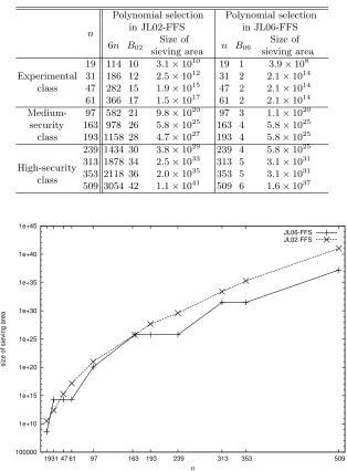
We compare JL06-FFS with JL02-FFS with respect to the size of the sieving area in the collection of relations step in three classes of extension degree n: exper-imental class as {19,31,47, 61}, medium-security class as {97,163,193}, and
high-security classas {239,313,353, 509}. Table 1 lists the smoothness bound and size of the sieving area in each variant. For eachn, we obtain the smooth-ness bound B02 in Equation (9) and B06 in Equation (10), and estimate the
size of the sieving area by Equation (8) in JL02-FFS and by Equation (11) in JL06-FFS.
Table 1.Parameters and sieving area
n
Polynomial selection in JL02-FFS
Polynomial selection in JL06-FFS
6n B02 Size of
sieving area n B06
Size of sieving area
Experimental class
19 114 10 3.1×10¹⁰ 19 1 3.9×10⁸ 31 186 12 2.5×10¹² 31 2 2.1×10¹⁴ 47 282 15 1.9×10¹⁵ 47 2 2.1×10¹⁴ 61 366 17 1.5×10¹⁷ 61 2 2.1×10¹⁴
Medium-security
class
97 582 21 9.8×10²⁰ 97 3 1.1×10²⁰
163 978 26 5.8×1025 163 4 5.8×1025 193 1158 28 4.7×1027 193 4 5.8×1025
High-security class
239 1434 30 3.8×1029 239 4 5.8×1025
313 1878 34 2.5×1033 313 5 3.1×1031 353 2118 36 2.0×1035 353 5 3.1×1031
509 3054 42 1.1×1041 509 6 1.6×1037
100000 1e+10 1e+15 1e+20 1e+25 1e+30 1e+35 1e+40 1e+45
19 31 47 61 97 163 193 239 313 353 509
size of sieving area
n
JL06-FFS JL02-FFS
Figure 1 shows the size of the required sieving area over GF(36n). The
siev-ing area in JL06-FFS is much smaller than that in JL02-FFS whenn̸= 31,163. Moreover, the differences between the sieving areas in JL06-FFS and in JL02-FFS increase along with the increase in n. The computational cost in the col-lection of relations step is closely related to the size of the sieving area, so the collection of relations step in JL06-FFS might be several times faster than that in JL02-FFS.
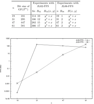
We have conducted experiments on the collection of relations step in JL02-FFS and JL06-JL02-FFS to confirm the difference between their computational costs of that step. Parameters in JL02-FFS and JL06-FFS are listed in Table 2. The curves that we used in our experiments are superelliptic ones, but notCabcurves
as [12] Note that we have only experimented with the experimental class as
n∈ {19,31,47,61}, not with medium and high-security classes.
Table 2.Parameters in our experiments
n Bit size of GF(36n)
Experiments with JL02-FFS
Experiments with JL06-FFS
6n B02 H02(x, y) n B06 H(x, y)
19 181 114 10 y4+x 19 1 y5+x
31 295 186 12 y4+x 31 2 y4+x 47 447 282 15 y4+x 47 2 y5+x
61 581 366 17 y5+x 61 2 y6+x
1e-05 0.0001 0.001 0.01 0.1 1 10 100 1000
19 31 47 61
time (day)
n
JL06-FFS JL02-FFS
In our experiments, we used 96 cores, each of which had the same performance about Intel 2.83GHz Xeon. We implemented the lattice sieve [26] in JL02-FFS as [12, 15, 16]. On the other hand, we implemented the polynomial sieve [10] in JL06-FFS, since we fixed r as a monic poynomial in the collection of relations step and so the lattice sieve might not be efficient. The details of our implementation in JL06-FFS are described in Section 4.
Figure 2 shows the time complexity of JL02-FFS and JL06-FFS to com-pute the entire sieving area in the collection of relations step in GF(36n) with n= 19,31,47,61, respectively. Note that we estimated the time when the com-putation lasts over one hour.
Whenn = 19,61, our implementation on JL06-FFS is faster than that on JL02-FFS, and we confirm that JL06-FFS is more efficient than JL02-FFS for solving the DLP in GF(36n). In particular, when n = 61, our implementation of JL06-FFS takes about 66 days for the collection of relations step, but our implementation of JL02-FFS takes about 165 days for the same step. Therefore, the former is 2.5 times faster than the latter. Accordingly, we expect that JL06-FFS will be efficient for solving the DLP in GF(36n) for largern.
4
Solving the DLP in GF(3
6·71)
In this section, we report that the DLP in GF(36·71) of 676-bit size is solved
by improving JL06-FFS. In our implementation, we deal with four practical improvements, polynomial sieve, free relation, Galois action, and parallel Lanczos method.
Particularly, by using the polynomialH(x, y) =y6+x, we only need to find about 1/8 of the originally required relations in the collection of relations step. Furthermore, via the Galois action, the size of the matrix given by the relations is also decreased to 1/6 of the original. To the best of our knowledge, the 676-bit size is currently the record for solving the DLP in GF(36n).
4.1 Collection of Relations
In the collection of relations step, we collect many double smooth pairs (r, s). The simple idea for collecting them is factoring Equations (2) and (3) for all pairs (r, s). This is not practical since we have to factor them about (36)B×(36)B+1
times. In order to reduce the number of factorings, we use a sieving method. The idea of sieving is merely factoring Equations (2) and (3) of the pair (r, s), which has a high probability of becoming a double smooth pair. Such a pair is called a candidate.
The polynomial sieve [10] and the lattice sieve [26] are well-known sieving algorithms. Although the lattice sieve has been implemented in some experiments of the FFS [12, 15, 16], we implemented the polynomial sieve sinceris fixed as a monic polynomial by the polynomial sieve in JL06-FFS, whereas neither rnor
Polynomial Sieve We describe the polynomial sieve in Equation (2), namely,
rm+s. Notice that we can also sieve in Equation (3) with the same procedure. Moreover, we discuss the case where s is fixed and omit the details when r is fixed. By fixed s, we can leadr such thatrm+sis divisible by p∈BR or its power, where the degree of p is not larger than B. Additionally,rm+s+kp
with k∈ GF(36)[x] is also divisible by p. Hence, we can obtain all r of degree
less than or equal toB such thatrm+sis divisible byp. After computing such all r for each p, we can obtain the pair (r, s) such thatrm+s is divisible by some p. If the summation of the degree of allp, which divide rm+s, reaches deg(rm+s), thenrm+shas a high probability of becomingB-smooth and the pair (r, s) becomes a candidate.
In this procedure, the most time-consuming work is to computer+kp for allk∈GF(36)[x] whose degree is not larger thanB. In characteristic two,
Gor-don and McCurley proposed a method using binary gray codes [10] to compute theser+kp. Using ternary gray codes, we can also compute them efficiently in characteristic three.
In the polynomial sieve, we sieve with all powers of p whose degree is not larger than B. Since B is very small, such as 1 or 2 in JL06-FFS, the power of p is only p2 when deg(p) = 1. Such polynomials are exceptional since there are 36 monic irreducible polynomials of degree 1 in GF(36)[x]. In this way, we can obtain only candidates each of which generates a relation in Equation (5) (except thatrandsare not relatively prime). Thus, we only check the greatest common divisor of r and s, but not the smoothness of Equations (2) and (3) using theB-smooth test [10].
Free Relation By considering how a divisor⟨p⟩inBRis factorized into divisors in GF(36)[x, y]/(H), namely, obtaining the following congruent expression that
H(x, y)≡
d
∏
i=1
(y−ti) (modp),
wheredis the degree ofH(x, y) ony, we can obtain a relation virtually for free, without the sieving procedure. We call such a relation a free relation.
The number of free relations depends on the degreedofH(x, y) onyand the characteristic of the field treated in the FFS. In fact, there are about #BA/dfree
relations in many cases and, furthermore, they increase when the characteristic is small. For example, in the case of GF(36n) andH(x, y) =y6+x, there are
about #BA/2 free relations sincey6+xis generally factored as (y−t
1)3(y−t2)3
modulop.
4.2 Linear Algebra
equation modulo (36n−1)/(36−1), by applying the parallel Lanczos method
described as [3]. In this section, we describe the Galois action and our ideas about parallel computation of the matrix operation.
Galois Action Here, we consider to reduce unknowns of linear equations, using the Galois action which was presented in [18].
Let M′ be the matrix given by the relations, whose row M′(i) means the i-th relation andj-th columnM′(j)corresponds to the factorbasepj. In order to
use the Galois action, we choose the polynomial f ∈GF(36)[x] satisfying that
all coefficients of f are in GF(3) and degf =n, then we construct GF(36n) as
GF(36)[x]/(f). Let ϕ be the Frobenius power such thatϕ(ξ) =ξ3n
. As ϕfixes the element xin GF(3)[x]/(f), we also haveϕ(x) =xin GF(36)[x]/(f) by the
assumption of f. However, for an element c ∈GF(36)\GF(3),ϕ does not fixc
in GF(36)[x]/(f) by the above assumption that n is coprime to 6. The monic
irreducible polynomialpj ∈BRof degree not larger thanB, and we assume that B = 1 for convenience. In fact,pj =x+cj wherecj ∈GF(36) sinceB = 1, so
we have
ϕ(pj) =ϕ(x+cj) =x+ϕ(cj)
in GF(36)[x]/(f). Ifcjis not in GF(3), it is clear thatcj≠ ϕ(cj) in GF(36)[x]/(f). This fact implies that there are ordinarily many unknowns of linear equations, which can be rewritten by the other one via the Galois action. Clearly, for such
pj, there existspj′ satisfying that
logγpj′ = logγϕ(pj) = 3nlogγpj (12)
wherepj ̸=pj′. Therefore, we can remove thej′-th columnM′ (j′)
and set thej
-th columnM′(j)asM′(j)+ 3nM′(j′). Then we denote the new matrixM∗ as the reducedM′. Notice that this technique is also used for the algebraic factorbase. Consequently, the number of unknowns is about 1/6 of the original; thus, the number of relations is reduced to about 1/6. In our implementation, we do not re-duce the factorbase in the sieving phase (the computation is the same as the case without the Galois action). After sieving, we compress obtained relations using rewritable elements of the factorbase via the Galois action as Equation (12), and so the factorbase is reduced to about 1/6. Using this procedure, we almost do not lose the probability of obtaining the relation. Hence, this technique enables us to perform computations for the collection of relations step about 6 times as fast as before, and the linear algebra step can be also done about 62times faster.
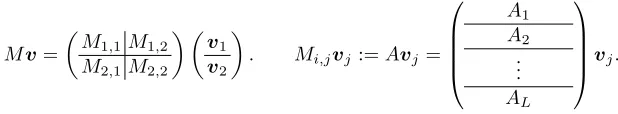
Parallel Lanczos method The reduced matrix M∗ is reconstructed to opti-mize first, then we apply the parallel Lanczos method to it. Before explaining the reconstruction, we begin with the explanation of the parallel computation. Assume that there are four nodes written asN1,1, N1,2, N2,1, N2,2and each node
vectorvis also partitioned intov1,v2, andvjis given to nodesNi,j, Ni′,j where i̸=i′. Moreover,Mi,j is partitioned intoLmatricesAℓ whenNi,j hasL cores.
Fig. 3. PartitioningM into four matrices Mi,j andMi,j intoLmatricesAℓ.
Mv = (
M1,1M1,2 M2,1M2,2
) (
v1 v2
)
. Mi,jvj:=Avj =
A1 A2
.. .
AL
vj.
We now give the notation of the Lanczos method. The Lanczos method can operate only a symmetric matrix; however, the given matrix M is usually non-symmetric. Therefore, we try to solve the linear equation of the formMTMv=
α, where v is an unknown column vector consisting of the logarithms of the factorbase andαis the given column vector. Note that computingMTM is not efficient, so we compute the vector u=Mv and MTu. For more details about this computation is in [22].
After partitioningM, we perform a parallel computation foru:=Mv and
w := MTu with Mi,j. Letv1, v2,u1, and u2 be the partitioned vectors such
thatv=v1⊕v2andu=u1⊕u2. From Algorithm 1, we obtain the partitioned vectorwi such thatw=wi⊕wi′ in nodeNi,j, wherei∈ {1,2} andi′= 3−i.
The symbolj′ also means thatj′ = 3−j forj∈ {1,2}.
Algorithm 1(Computation with nodeNi,j.)
Input : the partitioned matrixMi,j and the partitioned vectorvj.
Output : the partitioned vector wj such that w1⊕w2 = MTMv, where j is
equal to 1 or 2.
[Step for computation ofu:=M v] 1.ui,j :=Mi,jvj.
2. Giveui,j to Node Ni,j′ and receiveui,j′ fromNi,j′.
3.ui:=ui,j+ui,j′.
[Step for computation ofw:=MTu]
4.wi,j:=Mi,jT ui.
5. Givewi,j to NodeNi′,j and receive wi′,j from Ni′,j.
6.wj:=wi,j+wi′,j.
Lines 4, 5, and 6 describe the computation ofMTu. Note that in each nodeN i,j,
by regarding the column ofMi,jas the row ofMj,iT, we do not have to tradeMi,j
withMT
j,i, namely, we can cut unnecessary operations.
We have discussed the parallel computations among nodes, and now we move on to the parallel computations among cores in one node. Here,Aℓ denotes the partitioned matrix ofMi,jsuch thatMi,j=⊕Lℓ=1Aℓ. From Algorithm 2, we can easily obtain Aℓvj, and then we set the new vector ui,j = (A1vj, . . . , ALvj)T,
whereLis the number of cores in the same node. Similarly, we can easily obtain
ATℓui and computewi,j =
∑L
ℓ=1A T
Algorithm 2(Parallel computation ofMi,jvjamongLcores in the same node.)
Input : the partitioned matrixA:=Mi,j whose size iss×tand the partitioned
t-vectorvj.
Output : the partitioned vectorui,j such thatui,j=Avj.
1. Computebℓ:=Aℓvj forℓ= 1 toℓ=Lin parallel.
2.ui,j =⊕Lℓ=1bℓ.
Algorithm 3(Parallel computation ofMT
i,juiamongLcores in the same node.)
Input : the partitioned matrixA:=Mi,j whose size iss×tand the partitioned s-vectorui.
Output : the partitioned vectorwi,j such thatwi,j=ATui.
1. Computecℓ:=ATℓui forℓ= 1 toℓ=Lin parallel.
2.wi,j=
∑L
ℓ=1cℓ.
From the parallel computations ofMi,jvj and so on, we obtain the vector MTMv from Algorithm 1 and 2. Therefore, we need to reconstructM so that
each node has the balanced calculation amount of computing Mi,jvj and so
on. It is clear that the calculation amount depends on the number of non-zero elements in the allotted matrix, and the distribution of non-zero elements inM
is not uniformity. In fact, the number of non-zero elements in a column of M
is not balanced, but that in a row is balanced. Thus, we reconstruct the new matrixM so that the number of non-zero elements inM1,1 andM2,1 is almost
equal to that inM1,2andM2,2 by sorting columns ofM∗ defined in the section
of the Galois action. We perform a similar strategy as above for the parallel computation among cores in the same node, namely,A is partitioned into 4 or 8 smaller matricesAℓso that eachAℓ has almost the same number of non-zero elements.
4.3 Computation Results
In this section, we describe our computation results of the 676-bit DLP in GF(36·71), which contains a multiplicative subgroup whose order is a 112-bit prime. We construct GF(36) as GF(3)[z]/(z6+ 2z+ 2) and define a mapping
ψ : Z → GF(36)[x], such that ψ−1 : z 7→3, x 7→ 36, in order to represent the
element in GF(36)[x].
In the polynomial selection step, we setH(x, y) =y6+xin order to use the
Galois action. Moreover, we select m ∈ GF(36)[x] such that all its coefficients
are in GF(3) to construct f whose coefficients are also in GF(3). By an easy computation, we obtain propermandf as follows,
m=ψ(0x456bc 60e76c11 1e679735 c929fc55)
f =ψ( 0x9 2d3e5daf 5ac01130 4e6909f7 09cc8833 baa757d3
17dc6f99 9c8b98b5 ab8baa01 d68ec151 aec39e2e ed081c79
d851066b 3ffb2a4f a3e19c1e cef46675 0918a26d 9c7cacd4
Then, GF(36n) is constructed as GF(36)[x]/(f). When we set the smoothness
boundB= 2, there are 266,085 elements in the rational factorbase and 265,721 elements in the algebraic factorbase, so we need to collect at least 531,806 rela-tions. However, the size of the sieving area when B = 2 is too small to collect enough relations.
We settle this problem by using the Galois action, since we can considerably reduce the number of required elements in the factorbase described in Section 4.2. In fact, we need only 88,674 relations, and so this number is about 1/6 the number of the originally required relations.
Moreover, we deal with free relations which are obtained without sieving. If we chooseH(x, y) asy6+x, then it is fortunately factored as (y−t
1)3(y−t2)3
(mod p) for most of elements p in the factorbase, and so there are 132,860 (≈ #BA/2) free relations. Even if we delete many duplicates which are produced by using the Galois action, 22,155 free relations remain. Thus, we only have to find at least 66,519 relations in the collection of relations step, and this number is about 1/8 that of the originally required relations.
In the collection of relations step, we use the polynomial sieve described in Section 4.1 and compute relations using five nodes, each consisting of Intel
Quad-Core Xeon E5440 (2.83 GHz) × 2 CPUs with 16-GB RAM, one node
consisting of Intel Quad-Core Xeon X5355 (2.66 GHz) ×2 CPUs with 16-GB RAM, and twelve nodes, each consisting of Intel Quad-Core Xeon L5420 (2.33 GHz) ×1 CPU with 4-GB RAM, total of 96 cores. In 18 days of computation, after removing duplicates, we found 66,646 relations. Thus, we obtained a total of 88,801 relations, which are enough to solve the linear equation in Equation (7). The linear equation constructed from the relations has to be solved modulo (36·71−1)/(36−1); however, the Lanczos method may fail when the modulus
has a small prime factor. Therefore, we work modulo the factor Ni of (36·71−
1)/(36−1),
N1= (32·71+ 371+ 1)/(13·5113),
N2= (32·71−371+ 1)/(7·210019·49682251·55126531), N3= (371+ 1)/(22·853·2131·82219),
N4= (371−1)/2.
where every prime factor of Ni is larger than 30 bits andNi is relatively prime
to each other.
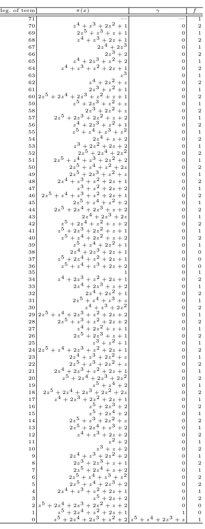
In the individual logarithm step, our target of computing the logarithm is the element
π(x) =ψ(⌊π×10202⌋)
= (z4+z3+ 2z2+ 1)x70+· · ·+ (z5+ 2z4+ 2z3+z2+ 2)
in basis γ =ψ(0x456). The complete value of π(x), γ and f is written in Ap-pendix. We choose the representation ofπ(x) as a product of elements of degree at most 7 as follows:
γτπ(x)≡z1/z2 (modf), where
z1=ψ(0x333)×ψ(0x345)×ψ(0x427)×ψ(0x43b)×ψ(0x4c3) ×ψ(0xd909 66c7e3ec)×ψ(0x293996d cc380672)
×ψ(0x3ff378e 3d4659d0)×ψ(0x6 27d6c281 0a0fc5a2)
×ψ(0x8 f4797e29 a9ec3b4a),
z2=ψ(0x318)×ψ(0x45 4c6fbfd4)×ψ(0x54 c69e6f97) ×ψ(0x1686d 42782189)×ψ(0x3cf67a5 84055cd8)
×ψ(0x8 f68ab2e2 5d2bc04f)×ψ(0xb cc56922c f651b383),
τ = 0x2 0f822e8c ac48792a e2aea337 c9002b49 bbf1b864
43a6111b 24c5593d e44daf43 e26de26e 1f85f982 1ba485b3
beda74bd f782626d 6cd38bb2 8f829867 5dc04adc f8741c24,
andz1, z2are 7-smooth. Then, we compute the logarithms ofz1andz2in basis γusing the special-qdescent technique [16, 18]. With about 14 days computation using five nodes, each consisting of Intel Quad-Core Xeon E5440 (2.83 GHz)× 2 CPUs with 16-GB RAM, and one node consisting of Intel Quad-Core Xeon X5355 (2.66 GHz)×2 CPUs with 16-GB RAM, we compute the logarithms,
logγz1≡ 0x3 fc71c577 10be8e3f e7af0fba e00e711f 0ad6dd50
38fb8f26 c0fadb3b 448cab2f 67671247 285f9e95 dc501717
d9def844 a75f9e58 f04a9bd2 3a5d0fdb 8f8ebb9f fea4deea,
logγz2≡ 0x4 82febaec ae4382e0 e651f577 09df4e7d 99d99d34
03db5d5e 521c4e2b da89ec33 6c9d45d6 2dd1f982 2f198fb2
6c069414 3b0b1544 ece8e4b1 5304872f 6ff261fd 03b271c7.
moduloN, and so we obtain logγπ(x) modN.
The logarithm in multiplicative subgroups of less than 30 bits are computed using the Pollard’sρmethod in a minute. Using the Pohlig-Hellman method, we compute the logarithm logγπ(x):
logγπ(x) = 0x8 78b54797 2fb6ff9b 57add5d5 11f69de6 a3853f98
68d53cc0 5b531076 2872ac6a 320874bf ba6d66d6 8e5e245f
39778f02 31ae791a acbab8c7 5ee6850c 9f5df0e5 f6b8ab0b
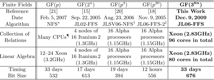
Table 3.Records for solving the DLP in finite fields
Finite Fields GF(p) GF(2n) GF(p3) GF(p30) GF(36n)
Reference [21] [15] [20] [18] This Work
Date Feb. 5, 2007 Sep. 22, 2005 Aug. 23, 2006 Nov. 9, 2005 Dec. 9, 2009
Algorithm NFS⋆ JL02-FFS JLSV06-NFS†JL06-FFS-2‡ JL06-FFS
Collection of
Relations Many CPUs¶
4 nodes of 16 Itanium 2
(1.3GHz)
16 Alpha processors (1.15GHz)
16 Alpha processors (1.15GHz)
Xeon (2.83GHz) 96 cores in total
Linear Algebra 12–24 Xeon (3.2GHz)
4 nodes of 16 Itanium 2
(1.3GHz)
16 Alpha processors (1.15GHz)
16 Alpha processors (1.15GHz)
Xeon (2.83GHz) 80 cores in total
Timing 33 days 17 days 19 days 12 hours 33 days
Bit Size 532 613 394 556 676
⋆NFS: Number Field Sieve [9, 17].†JLSV06-NFS: NFS in the medium prime case [20].
‡See footnote2on page 2. ¶There are no detailed descriptions of computational resources in [21].
and completely solve the DLP in GF(36·71) of 676-bit.
4.4 For Larger Extension Degrees
We have solved the DLP in GF(36n) fornin the experimental class, where the
smoothness bound B (i.e., B06) is less than or equal to 2 (ref. Table 1). Note
that the size of the sieving area increases (36)2-fold if the smoothness bound B increases by one (see Equation (11)). However, we expect that, if we set
B = 3, the DLP in GF(36·97) might be computed for several years by using
dozens of our computational resources through various techniques such as large prime variation, block sieving and sieving via bucket sort [29, 4], and SIMD implementation.
5
Concluding Remarks
In this study, we implemented a new variant of the FFS in GF(36n) (n is a
prime), proposed by Joux and Lercier in 2006 [18], and compared it with the earlier variant, which was also proposed by Joux and Lercier in 2002 [16] with practical experiments. In solving the DLP in GF(36n), these two variants of the
FFS have the same asymptotic complexity, but we expected the new variant to be more efficient than the earlier one in some extension degrees n. From our experimental results, we confirmed this forecast when the extension degree
n = 19,61. Moreover, with our implementations, we succeeded in solving the DLP in GF(36·71) of 676-bit size with about 33 days computation.
an open problem to analyze the hardness of the DLP with practical key sizes in such finite fields.
References
1. L. M. Adleman. The function field sieve. ANTS-I, LNCS 877, pp. 108–121, 1994. 2. L. M. Adleman and M.-D. A. Huang. Function field sieve method for discrete
logarithms over finite fields. Inform. and Comput., Vol. 151, pp. 5–16, 1999. 3. K. Aoki, T. Shimoyama, and H. Ueda. Experiments on the linear algebra step in
the number field sieve. IWSEC 2007, LNCS 4752, pp. 58–73, 2007.
4. K. Aoki and H. Ueda. Sieving using bucket sort.ASIACRYPT 2004, LNCS 3329, pp. 92–102, 2004.
5. P. S. L. M. Barreto, S. Galbraith, C. ´O h ´Eigeartaigh, and M. Scott. Efficient pairing computation on supersingular abelian varieties. Des., Codes Cryptogr., Vol. 42, No. 3, pp. 239–271, 2007.
6. J.-L. Beuchat, N. Brisebarre, J. Detrey, E. Okamoto, M. Shirase, and T. Takagi. Algorithms and arithmetic operators for computing theηT pairing in characteristic
three. IEEE Trans. Comput., Vol. 57, No. 11, pp. 1454–1468, 2008.
7. D. Boneh, D. Crescenzo, R. Ostrovsky and G. Persiano. Public key encryption with keyword search. EUROCRYPT 2004, LNCS 3027, pp. 506–522, 2004. 8. D. Boneh and M. Franklin. Identity based encryption from the Weil pairing.SIAM
J. Comput., Vol. 32, No. 3, pp. 586–615, 2003.
9. D. M. Gordon. Discrete logarithms in GF(p) using the number field sieve. SIAM J. Discrete Math., vol. 6, no. 1, pp. 124-138, 1993.
10. D. M. Gordon and K. S. McCurley. Massively parallel computation of discrete logarithms. CRYPTO’ 92, LNCS 740, pp. 312–323, 1992.
11. R. Granger. Estimates for discrete logarithm computations in finite fields of small characteristic. Cryptography and Coding 2003, LNCS 2898, pp. 190–206, 2003. 12. R. Granger, A. J. Holt, D. Page, N. P. Smart, and F. Vercauteren. Function field
sieve in characteristic three. ANTS-VI, LNCS 3076, pp. 223–234, 2004.
13. R. Granger, D. Page, and M. Stam. Hardware and software normal basis arith-metic for pairing-based cryptography in characteristic three. IEEE Trans. Com-put., Vol. 54, No. 7, pp. 852–860, 2005.
14. D. Hankerson, A. Menezes, and M. Scott. Software implementation of pairings. In
Identity-Based Cryptography, pp. 188–206, 2009.
15. A. Joux et al. Discrete logarithms in GF(2607) and GF(2613). Posting to the
Number Theory List, available athttp://listserv.nodak.edu/cgi-bin/wa.exe? A2=ind0509&L=nmbrthry&T=0&P=3690, 2005.
16. A. Joux and R. Lercier. The function field sieve is quite special. ANTS-V, LNCS 2369, pp. 431–445, 2002.
17. A. Joux and R. Lercier. Improvements to the general number field sieve for discrete logarithms in prime fields. A comparison with the Gaussian integer method. Math. Comp., Vol. 72, No. 242, pp. 953–967, 2002.
18. A. Joux and R. Lercier. The function field sieve in the medium prime case. EU-ROCRYPT 2006, LNCS 4004, pp. 254–270, 2006.
20. A. Joux, R. Lercier, N. P. Smart, and F. Vercauteren. The number field sieve in the medium prime case. CRYPTO 2006, LNCS 4117, pp. 326–344, 2006.
21. T. Kleinjung et al. Discrete logarithms in GF(p) - 160 digits. Posting to the Number Theory List, available athttp://listserv.nodak.edu/cgi-bin/wa.exe? A2=ind0702&L=nmbrthry&T=0&P=194, 2007.
22. B. A. LaMacchia and A. M. Odlyzko. Solving large sparse linear systems over finite fields. CRYPTO’ 90, LNCS 537, pp. 109–133, 1991.
23. R. Matsumoto. UsingCabcurves in the function field sieve. IEICE Trans. Funda-mentals, Vol. E82-A, pp. 551–552, 1999.
24. A. J. Menezes, T. Okamoto and S. Vanstone. Reducing elliptic curve logarithms to logarithms in a finite field. IEEE Trans. Inform. Theory, Vol. 39, No. 5, pp. 1639–1646, 1993.
25. D. Page, N. P. Smart, and F. Vercauteren. A comparison of MNT curves and supersingular curves. Appl. Algebra Engrg. Comm. Comput., Vol. 17, No. 5, pp. 379–392, 2006.
26. J. Pollard. The lattice sieve. InThe Development of the Number Field Sieve, pp. 43–49, 1991.
27. C. Pomerance and J. W. Smith. Reduction of huge, sparse matrices over finite fields via created catastrophes. Experiment. Math., Vol. 1, No. 2, pp. 89–94, 1992. 28. O. Schirokauer. The special function field sieve. SIAM J. Discrete Math., Vol. 16,
No. 1, pp. 81–98, 2003.
29. G. Wambach and H. Wettig. Block sieving algorithms. Technical Report 190, Informatik, Universit¨at zu K¨oln, 1995.
Appendix A: Some Solutions of the DLP in GF(3
6·71)
We present some solutions (discrete logarithms) in factorbase used in our im-plementation for solving the DLP in GF(36·71). We have found 66,646 relations satisfying Equation (5). We give one of them as an example,
6
∑
i=0
logγpi≡ 4
∑
j=0
3 logγκj (mod (36·71−1)/(36−1)), (13)
where eachpi is in rational factorbase,
p0=ψ(0x2d9), p1=ψ(0x90581), p2=ψ(0x9ea2b), p3=ψ(0xb1a07),
p4=ψ(0xb942e), p5=ψ(0xcada1), p6=ψ(0xd6d36),
and eachκjcorresponding to an element in algebraic factorbase by Equation (6)
is given as follows,
κ0: ⟨ψ(0x3c3), y−ψ(0x175)⟩, κ1: ⟨ψ(0x3c4), y−ψ(0x200)⟩, κ2: ⟨ψ(0x533), y−ψ(0x258)⟩, κ3: ⟨ψ(0xda9c2), y−ψ(0x4cc58)⟩, κ4: ⟨ψ(0xed6e4), y−ψ(0x387b6)⟩.
By the Galois action, we have
p6≡p333·71 (modf), κ4≡κ3
3·71
3 (modf),
and so we can removep6andκ4 from unknowns of Equation (7).
LetNbe the product of prime factors of (36·71−1), where those prime factors
are not larger than 55,126,531 (Note thatN is a 602-bit integer). Equation (13) also holds modulo N instead of (36·71−1)/(36−1), and so we obtain the
fol-lowing solutions of Equation (13) moduloN except for logγp6and logγκ4, after
performing the linear algebra step:
logγp0≡ 0x8 9e0c0faa 4190baa5 c885e3b7 308ae498 eb2d4a03
0dfab3d9 16437d96 bfd4e2b9 014f5402 90aa2f83 7b9cc76b
16ae97ef dcc9c319 670f0f9c 47e8ea96 4754cfbf 1529c311,
logγp1≡ 0x2 e8b84752 70de651a b03ae702 e3268e86 77179013
0c9edab5 31d2ac5b 2a23da92 2e8352c5 321832bf ff36a8d5
2d16c9e5 ae47c6fc 2ba7a1c5 cc990233 34c3d6da 25e08d52,
logγp2≡ 0x7 b565cae8 39dc8d83 415b0b9e 164c7b55 6e57ad98
80b8f232 7cf30ebe 972ac1fb 2d1133be 5cdd9604 c9ea6e83
logγp3≡ 0x6 ae81aef6 7c0fddcf 7c23e69e c3f18e07 bf546751
8df9d1ad 78113a85 9a2578c8 36764402 2598160b 5c055ed4
7d412a42 17c987c0 14aafff7 03ef6fa4 c6771dfd 150b88f2,
logγp4≡ 0x7 2e418546 92ba2b75 8d0831df 1d5ca5c0 f6d8a05d
0528c97d 16c4f782 d9b59ce7 d55deefe bf85390a 23113680
b184d203 d1d3b6a4 e9d9263a 8544acd7 5afc9974 78a4498a,
logγp5≡ 0x1 c35f26bf 717ed338 cfd71243 b86c024b 98b18342
4710450a d9aaf2e3 557ce5ed debbc870 0fc840f2 19aca778
2ba931a2 cdd2cb53 a2dafcaa 28a5176e a378bf8c 9a6cd33c,
and,
logγκ0≡ 0x 92671082 6cf3288f 1c83edcf 66fb9041 9bb2239c
10cd8445 820d975e 6f9730fb f4ca3005 279a500d b2fc0f60
b4425edb 65991a31 629d54e7 84ae64b6 080828b3 0fc6ba0b,
logγκ1≡ 0x7 06c2cfcd 7fb4f7c8 386ea65b c0c259c3 f14888ec
ccda75ee 77ddddf4 065a7da6 981af728 98699166 c52484c6
73bbefbd a4660135 1244b297 42f3cf76 fdab7cad 3d01e8a1,
logγκ2≡ 0x5 4623bf43 0ede6e43 bbe3cb8b a79c1400 97f7ac1e
2320c70e 5a700159 4460b073 e5c670c5 d19921ea 59f4f9c6
41ce8203 28edb204 94bd322f 3551d5ee 472cf59b d58d0bd0,
logγκ3≡ 0x6 e063f01c 43624c96 30712701 2223edf3 95ddfdc2
aa1dd9f6 dd3636ef 12d9260f 555a2101 c0e94fe5 9a524c5b
c2c1d768 1499d7b6 41b71d4f b13566b3 b39794c5 90ff78cb,
modN. Finally, by the Galois action, we obtain that
logγp6≡33·71logγp3≡
0x7 3deb8075 ee684576 073761e2 974c4eba 72df97ce
299f9e46 87ae3f70 b6cd8b50 1c65ccb3 e9ed8f80 08387efe
9326eea8 7302c1a5 1f0671b5 22e32949 81250923 9b072989,
logγκ4≡33·71logγκ3≡
0x4 0473a949 4056ac7c 76677e6f a284977a 2a2e539f
751d5e0b ee628ca8 63e7f732 a02886c2 0711d445 0006c79a
778c6fbf abb923e7 e89deb8d 0c7f5508 2d797bd2 2414eaa1,
modN.
Appendix B: Complete Value of Elements
Table 4.Complete Value ofπ(x), γandf
deg. of term π(x) γ f
71 — — 1
70 z4 +z3 + 2z2 + 1 0 2
69 2z5 +z3 +z+ 1 0 1
68 z4 +z3 + 2z+ 1 0 2
67 2z4 + 2z3 0 1
66 2z3 + 2 0 2
65 z4 + 2z3 +z2 + 2 0 1
64 z4 +z3 +z2 + 2z+ 1 0 2
63 z3 0 1
62 z4 + 2z2 +z 0 2
61 2z3 +z2 + 1 0 1
60 2z5 + 2z4 + 2z3 +z2 +z+ 1 0 2
59 z5 + 2z3 +z2 +z 0 1
58 2z3 + 2z2 +z 0 2
57 2z5 + 2z3 + 2z2 +z+ 2 0 1
56 z4 + 2z3 +z2 + 1 0 2
55 z5 +z4 +z3 +z2 0 1
54 2z4 +z+ 2 0 2
53 z3 + 2z2 + 2z+ 2 0 1
52 2z5 + 2z4 + 2z2 0 2
51 2z5 +z4 +z3 + 2z2 + 2 0 1
50 2z5 +z4 +z2 + 2z 0 2
49 2z5 + 2z3 +z2 +z 0 1
48 2z4 +z3 +z2 + 2z+ 1 0 2
47 z3 +z2 + 2z+ 2 0 1
46 2z5 +z4 +z3 +z2 + 2z+ 1 0 2
45 2z5 +z4 +z2 + 2 0 1
44 2z5 + 2z4 + 2z3 +z+ 2 0 2
43 2z4 + 2z3 + 2z 0 1
42 z5 + 2z4 +z2 +z+ 2 0 2
41 z5 + 2z3 + 2z2 +z+ 1 0 1
40 z5 +z4 + 2z2 +z+ 2 0 2
39 z5 +z4 + 2z2 + 1 0 1
38 2z4 + 2z3 + 2z+ 1 0 0
37 z5 + 2z4 +z2 + 2z+ 1 0 0
36 z5 +z4 +z3 + 2z+ 2 0 0
35 1 0 1
34 z4 + 2z3 +z2 + 2z+ 1 0 2
33 2z4 + 2z3 +z+ 2 0 1
32 2z4 + 2z2 + 1 0 2
31 2z5 +z4 +z3 +z 0 1
30 z4 +z3 + 2z2 0 2
29 2z5 +z4 + 2z3 +z2 + 2z+ 2 0 1
28 2z5 +z3 +z2 + 2z+ 2 0 2
27 z4 + 2z2 +z+ 1 0 1
26 2z5 + 2z3 +z+ 1 0 2
25 z3 +z2 + 1 0 1
24 2z5 +z4 + 2z3 +z2 + 2z+ 1 0 2
23 2z4 +z3 + 2z2 +z 0 1
22 2z5 +z3 + 2z2 +z 0 2
21 2z4 + 2z3 +z2 + 2z+ 1 0 1
20 z5 + 2z4 + 2z3 + 2z2 0 2
19 z5 +z4 + 2 0 1
18 2z5 + 2z4 + 2z3 + 2z2 + 2z 0 2
17 z4 + 2z3 + 2z2 + 2z+ 1 0 1
16 z5 + 2z3 + 2 0 2
15 z5 + 2z4 + 2 0 1
14 2z5 +z3 + 2z2 +z 0 2
13 2z5 + 2z4 +z3 + 2 0 1
12 z4 +z3 + 2z+ 2 0 2
11 z2 + 2 0 1
10 z3 +z+ 2 0 2
9 2z4 +z3 + 2z2 + 2 0 1
8 2z3 + 2z3 +z+ 1 0 2
7 2z5 + 2z4 +z+ 2 0 1
6 2z5 +z4 +z3 +z2 0 2
5 2z5 +z4 + 2z3 + 2 0 2
4 2z4 +z3 +z2 + 2z+ 1 0 1
3 z5 + 2z+ 2 0 2
2z5 + 2z4 + 2z3 + 2z2 +z+ 2 0 0
1 z5 + 2z4 +z2 + 2z+ 1 1 0