1515
A MODEL FOR ESTIMATING THE DISTRIBUTION OF FUTURE
POPULATION
Ben David Nissim
Department of Economics and Management, Emek Yezreel Academic College, Israel
Garyn-Tal Sharon
Department of Economics and Management, Emek Yezreel Academic College, Israel
ABSTRACT
In most counties, statistical authorities collect data on the number of deaths in each age group. These data enables the calculation of life expectancy as well as the calculation of death and survival probabilities for each age group. In this paper, we develop an easy-to-use tool to estimate the distribution of future survivors for each cohort. Such a distribution defines the probabilities for the number of survivors at a given future time. Many institutions can benefit from the estimation of the distribution of future survivors (e.g., pension funds, geriatric institutions and medical authorities in general). Thus, our paper contributes not only to the literature on the projection of mortality rates, but it also has significant practical implications.
© 2014 AESS Publications. All Rights Reserved.
Keywords: Distribution, Future survivors, Life expectancy, Cohort, Mortality rates, Projection.
Contribution/ Originality
This study uses new methodology for estimating future distribution of survivors. Estimating
the probability of surviving individuals in time T via the continuous normal distribution
solution requires a multiple-integral calculation. We suggest a compact model that allows doing the
calculation via a single integral over the density distribution function.
1. INTRODUCTION
In most counties, statistical authorities collect data on the number of deaths in each age group,
which enables the calculation of death probabilities (and survival probabilities) as well as the
calculation of life expectancy for each age group. However, a large degree of uncertainty is
associated with these future survival probabilities.
Booth and Tickle (2008) reviewed the history of mortality projections and identified three
main projection methodologies. The first methodology builds epidemiological models in order to Asian Economic and Financial Review
1516
explain particular causes of death or known risk factors (see, Alderson and Ashwood, 1985). The
second methodology defines a target life expectancy and then determines a path to that life
expectancy. Such an approach allows expert opinion to be factored into the statistical process (see
Pollard, 1987; Olshansky, 1988). The third methodology is extrapolation - a term given to the
forecasting of future mortality based on past patterns (see Lee and Carter, 1992; Milevsky and
Promislow, 2001; Brouhns et al., 2002; Dahl, 2004; Biffis, 2005; Renshaw and Haberman, 2006;
Schrager, 2006; Cairns et al., 2009).
Many institutions would be interested in and benefit from the estimation of the distribution of
future population. Such a distribution defines the probabilities for the number of survivors for each
cohort at any given time in the future.
First of all, pension funds would benefit from forecasting the distribution of the expected
number of survivors in cohorts passed retirement age. When a death of an insured individual
occurs, pension funds usually pay a given compensation to the family in addition to the
continuation of the post-death pension payments (payment level might be different relative to the
pre-death payments). Funds can use past records and documentations of death probabilities in order
to evaluate the number of expected deaths. However, there is a high probability that the actual
number of deaths would be much larger than the anticipated number (calculated by the
multiplication of the number of people in a cohort by their probability of dying). This means that
even if pension funds operate with an expected actuarial balance, they might end up extremely
unbalanced due to volatility in the expected forthcoming deaths. If pension funds could forecast the
distribution of the number of deaths for each cohort, it would improve their forecasting tools (by
using the confidence interval of the expected number of deaths instead of solely using the expected
value) and thus will enable them to take steps to reduce their operational risks.
Insurance companies would also find it useful to evaluate the distribution of the future
expected number of survivors for each cohort since they are interested in estimating the
probabilities associated with their commitments, i.e., upcoming death compensation payments.
Although death probabilities enable the estimation of expected payments, they do not fully describe
the complete risks. For example, if the probability of dying for a given cohort is 2%, then the
expected number of deaths for 1,000 individuals (from this cohort) is 20. However, there is some
probability that more (and even much more) than 20 individuals will die, causing substantial losses
to the insurance company. The same considerations hold for deaths caused by car accidents
(drivers' insurance risks), earthquake insurance risks as well as health insurance risks.
Additionally, medical authorities would be interested in the same information. For example,
medical authorities evaluate death probabilities caused by epidemic diseases based on past records.
In particular, they are interested in the probability that the actual number of deaths would be much
larger than the expected number of deaths. Moreover, being exposed to a disease might create a
given risk of death in all future periods. Here again, the medical authority would benefit from
1517
A variety of approaches have been proposed for modeling randomness in the aggregation of
mortality rates over time. Lee and Carter (1992) worked with discrete time models and focused on
periodical application of stochastic mortality and its statistical analysis (see also Renshaw and
Haberman, 2006). Other researchers developed continuous time frameworks (see Dahl, 2004;
Schrager, 2006).
In this paper, we first assume that in each future period an agent faces a given likelihood to
survive. We assume that future annual survival probability is defined according to the report of the
realized death probabilities published by the statistical authorities. Then, we present a model that
enables the prediction of future survival distribution for each cohort.
2. THEORY/CALCULATION
2.1. Estimating the Distribution of Future Survivors for Each Cohort 2.1.1. The Bernoulli Distribution and the Binomial Distribution
Let us assume that individuals were born in period 0. According to statistical authorities,
their survival probability during period 1 is
p
1. That probability can be found in mortality ratestables published by the authorities. We can refer to the survival distribution at age 1 as a Bernoulli
distribution. Each agent faces a "successful trial" with probability
p
1 (survival) and a failure with aprobability
1
p
1 (death). Using the Newton Binomial formula, we can calculate the probability)
(
1
j
prob
that j agents will survive at age t=1, for j = 0,1,2,… . As , the binomialdistribution function is expressed in terms of the standard normal distribution function.
Using the same idea, the distribution of the number of survivors in period t depends on the
realized number of survivors in period t-1, . Thus, given the distribution of the number of
survivors in time t-1, we can calculate the distribution of the number of survivors in the following
period. Each individual faces a survival probability
p
t during period t, and, given thatindividuals survived period t-1, any j surviving agents face a survival probability
prob
t(
j
|
N
t-1)
in time t. The surviving agents face in time t+1 a new individual survival probability
p
t1 and,given that individuals survived period t, a new Bernoulli trial with survival probability
)
N
|
(
t1
j
1518 2.1.2. An Example: The Binomial Distribution
In order to simplify the presentation, let us assume that we estimate the distribution of survival
of a nonhuman species with survival probabilities of
p
1 andp
2 at years 1 and 2, respectively.Assuming that only N=3 objects were born in year zero, table 1 below shows the calculations of the
future survival distribution of the objects born in year 0, according to the Bernoulli distribution.
Table-1-Panel-A. The survival distribution in year 1 and in year 2 (given the number of survivors in year 1)
Number of survivors in year 1
Year 1 survival probability
Number of survivors in year 2
Year 2 survival
Probability given the number of survivors in year 1
0 1 3
0
1 (1 )
0 3 p p
0 1
1 1 2
1
1 (1 )
1 3 p p 0 1 2 0 2 (1 )
0 1 p p
1 2 0
1 2(1 )
( 1 1 p p
2 1 1
2
1 (1 )
2 3 p p
0 2 2
0
2 (1 )
0 2 p p
1 2 1
1
2(1 )
1 2 p p
2 0
2 2
2 (1 )
2 2 p p
3 1 0
3
1 (1 )
3 3 p p
0 2 3
0
2 (1 )
0 3 p p
1 2 2
1
2(1 )
1 3 p p
2 2 1
2
2 (1 )
2 3 p p
3 2 0
3
2 (1 )
3 3 p p
Notice that the survival probability in year 2 (table 1 - panel B) is the product of the probability
of j survivors in year 1, j=0,1,2,3, multiplied by the probability of k survivors in year 2, such that k
is lower than or equal to j. For example, the probability that j=2 objects survive year 1 and k=1
object survives year 2 is:
1 2 1 2 1 1 2
1 (1 )
1 2 * ) 1 ( 2 3 p p p
p
1519
1 1 2
1 (1 )
2 3 p p
is the probability that 2 people survive year 1 and
) 1 ( 1 2 2 1 2 p p
is the probability that 1 person survives year 2 given that 2 people had survived year 1.
Based on table 1, the overall survival distributions in years 1 and 2 are presented in table 2. The
year 1 survival probabilities are similar to those presented in panel A of table 1. The year 2 survival
Table-1–Panel-B. Survival distribution in year 2
Number of survivors in year 1
Number of survivors in year 2
Year 2 overall survival probability given the number of survivors in year 1
0 0 1 3
0
1 (1 )
0 3 p p 1
0 1
2 0 2 2 1 1
1 (1 ) 0 1 * ) 1 ( 1 3 p p p
p
1 0
2 1 2 2 1 1
1 (1 ) 1 1 * ) 1 ( 1 3 p p p
p
2
0 22
0 2 1 1 2
1 (1 )
0 2 * ) 1 ( 2 3 p p p
p
1 1
2 1 2 1 1 2
1 (1 )
1 2 * ) 1 ( 2 3 p p p
p
2 0
2 2 2 1 1 2
1 (1 )
2 2 * ) 1 ( 2 3 p p p
p
3
0 2 3
0 2 0 1 3
1 (1 )
0 3 * ) 1 ( 3 3 p p p
p
1 2 2
1 2 0 1 3
1 (1 )
1 3 * ) 1 ( 3 3 p p p
p
2 21
2 2 0 1 3
1 (1 )
2 3 * ) 1 ( 3 3 p p p
p
3 20
3 2 0 1 3
1 (1 )
3 3 * ) 1 ( 3 3 p p p
p
probabilities are calculated as follows. For each possible number of survivors k (k=0,1,2,3) in
period t=2, we take into consideration all possible number of survivors j in the preceding period (time 1), jk jk,...N0 , and then we sum these probabilities of the different scenarios
leading to k survivors in time 2:
0 ( )* ( ) ) ( N k j j k p j p k p .
1520 (1) 2 2 1 2 0 1 3 1 1 2 1 2 1 1 2 1 0 2 1 2 2 1 1
1 (1 )
1 3 * ) 1 ( 3 3 ) 1 ( 1 2 * ) 1 ( 2 3 ) 1 ( 1 1 * ) 1 ( 1 3 p p p p p p p p p p p
p
Prob of one survivor Prob of 2 survivors Prob of 3 survivors
in period 1 in period 1 in period 1
2.1.3. An Example: The Binomial Distribution – A Numerical Solution
Let us now continue the binomial distribution example from section 1.1.1. As an example,
given
p
1
0
.
96
and 3 2 2p , the survival distribution in years 1 and 2 are presented in table 3.
Table-2. The overall Survival distribution in years 1 and 2
Number of survivals
Year 1 survival probability
Year 2 survival probability
0 3
1 0 1(1 ) 0 3 p p 3 2 0 2 0 1 3 1 2 2 0 2 1 1 2 1 1 2 0 2 2 1 1 1 3 1 0
1 (1 )
0 3 * ) 1 ( 3 3 ) 1 ( 0 2 * ) 1 ( 2 3 ) 1 ( 0 1 * ) 1 ( 1 3 ) 1 ( 0 3 p p p p p p p p p p p p p
p
1 2
1 1 1(1 )
1 3 p p 2 2 1 2 0 1 3 1 1 2 1 2 1 1 2 1 0 2 1 2 2 1 1
1 (1 )
1 3 * ) 1 ( 3 3 ) 1 ( 1 2 * ) 1 ( 2 3 ) 1 ( 1 1 * ) 1 ( 1 3 p p p p p p p p p p p
p
2 1
1 2 1 (1 )
2 3 p p 1 2 2 2 0 1 3 1 0 2 2 2 1 1 2
1 (1 )
2 3 * ) 1 ( 3 3 ) 1 ( 2 2 * ) 1 ( 2 3 p p p p p p p
p
3 0
1 3 1(1 )
3 3 p p 0 2 3 2 0 1 3
1 (1 )
3 3 * ) 1 ( 3 3 p p p
p
Table-3. The survival distribution in years 1 and 2 given that
p
1
0
.
96
and3
2
2
p
2.2. The Normal Distribution
In order to ease the calculations, we can use the principle that as , the binomial
distribution function is expressed in terms of the standard normal distribution function.
Suppose is the number of surviving individuals at the end of time t-1,
p
t is theprobability of surviving the upcoming period t and is a random variable representing the number
Number of survivors Year 1 survival probability Year 2 survival probability
0 6.40E-05 0.046656
1 0.004608 0.248832
2 0.110592 0.442368
1521
of surviving individuals at the end of the period t. Then ) and as
, .
We define:
– the PDF (density distribution function) for the normal distribution. – initial number of individuals in time 0.
– the required number of surviving individuals in time T.
– a random variable, normally distributed, represents the number of surviving individuals in
time t.
– the realized number of surviving individuals in time t.
- the probability of surviving in time t.
The implementation of these definitions yields that represents the number of surviving
individuals in time 1 and is normally distributed:
( )
In general, the normal distribution for depends on – the realized number of surviving
individuals in time t-1. For t=2,3,…,T, this distribution of given is:
( )
The PDF of is:
√
while the PDF of is:
√
For simplicity, we start with a simple example, the same as the example discussed in sections
1.1.1-1.1.2. Let us describe the probability for 1 surviving individual in time 2. We substitute T=2
and and get that:
( )
( )
Thus, the probability for 1 surviving individual in time 2 is:
∫
∫
Note that equation (10) includes two terms: the external integral represents the probability for
the number of survivors in time 1, and the internal integral represents the probability that only one
individual will survive in period 2. Thus, we can further subdivide equation (10) into:
∫ ∫ ∫ ∫ ∫ ∫ ∫ ∫
1522
Given that
p
1
0
.
96
and3
2
2
p
, we use equation (10) for calculating the survivaldistributions in year 2, and the results are as follows: the probability for 1 survivor in period 2 is
0.26449, the probability for 2 survivors in period 2 is 0.437144, and the probability for 3 survivors
in period 2 is 0.184538. These numbers are similar in magnitude to those presented in Table 3. The
differences can be explained by the small sample of individuals.
Generalizing equation (10), we can express the probability of surviving individuals in time
T=2 as:
∫
∫
Placing the PDFs of and of , as defined by equations (6)-(9), into equation (12),
we get:
∫
∫
∫
√
∫
√
Note that after the internal integration over in equation (13), we get an expression that
depends on . Then, when integrating the external integration over , it does the integration also
over the that remained after the internal integration.
Now let us generalize the example above to T time periods and survivors in time T. We get
that the probability of survivors in time T is:
∫
∫
∫
∫
∫
Let us explain the underlying intuition of equation (14). The first part of equation (14) is:
∫ is the realized number of surviving individuals in time 1. We would like
to be lower than or equal to (since is the initial number of individuals in time 0, we cannot
have more surviving individuals in time 1 than the initial number of individuals in the time 0), but
greater than or equal to (since is the required number of surviving individuals in time T, we
cannot have less surviving individuals in time 1).
The second part of equation (14) is: ∫ We know now how many
individuals survived time 1: the answer is . Now we would like to consider the possible values
for - the realized number of surviving individuals in time 2. We would like to be lower than
1523
individuals in the time 1, the preceding period), but greater than or equal to (since is the
required number of surviving individuals in time T, T>2, we cannot have less surviving individuals
in time 2).
In general, we can explain what happens in time t. Part number t of equation (14) is:
∫ We know now how many individuals survived time t-1: the
answer is . Now we would like to consider the possible values for - the realized number of
surviving individuals in time t. We would like to be lower than or equal to (we cannot have
more surviving individuals in time t than the number of surviving individuals in the time t-1), but
greater than or equal to (since is the required number of surviving individuals in time T,
T>t, we cannot have less surviving individuals in time t).
The last part of equation (14) is: ∫
We know now how many
individuals survived time T-1: the answer is . We also know that - the realized number of
surviving individuals in time T – should equal to . Thus, the limits of the last integral of equation
(14) are: and . The result is the estimation of the probability of surviving
individuals in time T.
2.2.1. Another Example
We start with individuals in time 0. Let us describe the probability for 3 surviving
individual in time 3. We substitute , T=3 and and get that:
( ), ( ),
( ), ( )
Thus, given that , the probability for 3 surviving individual in time 3 is:
∫
∫
∫
∫
Let us explain the underlying intuition of equation (15). The first part of equation (15) is: ∫ is the realized number of surviving individuals in time 1. We would like to be lower than or equal to but greater than or equal to . Explanation: notice that since
we start with , the initial number of individuals in time 0, we cannot have more surviving
individuals in time 1. On the other hand, since is the required number of surviving
individuals in time 3, we cannot have less than surviving individuals in time 1.
The second part of equation (15) is: ∫ In time t=2, - the number of
individuals that survived period 1 - is given and known. Now we would like to consider the
possible values for - the realized number of surviving individuals in time 2. We would like to
be lower than or equal to but greater than or equal to . Explanation: since is the
1524
time 2. On the other hand, since is the required number of surviving individuals in time 3,
we cannot have less surviving individuals in time 2.
The explanation for the third part of equation (15) is similar.
The fourth and last part of equation (15) is: ∫ We know that - the realized
number of surviving individuals in time t – should be equal to . Thus, the limits of this last
part of equation (6) are: and . The result is the estimation of surviving
individuals in time 3.
In equation (16) we further decomposed equation (15) based on the following different
scenarios:
1). (this is the first line in the decomposition of equation (15).
2). (this is the second line in the decomposition of equation (15).
3). (this is the third line in the decomposition of equation (15).
4). (this is the fourth line in the decomposition of equation (15).
∫
∫ ∫
∫
∫
∫ ∫
∫
∫
∫ ∫
∫
∫
∫ ∫
∫
∫
∫ ∫
∫
2.3. Normal Distribution – The Compact Solution
Equation (14) in section 1.2 represents the continuous normal distribution solution. It estimates
the probability of surviving individuals in time T via T integrals, since it considers and accounts
for every realization regarding the number of surviving individuals that could occur. The first
integral goes over the possible values for the realized number of surviving individuals in time 1;
The second integral goes over the possible values for the realized number of surviving individuals
in time 2, given the realized number of survivors in period 1; Integral number t goes over the
possible values for the realized number of surviving individuals in time t, given the realized
number of survivors in period t-1; And the last integral, integral number T, estimates the
probability for exactly , the required number of surviving individuals in time T, given the
realized number of survivors in period T-1.
1525
of these T-1 integrals is explicit and simple: it is the calculation of the expected number of
surviving individuals in time T-1.
In order to avoid solving the problem via the multiple–integral solution as in equation (14), we
suggest another way to express the average expected number of individuals in time T-1, .
We define the probability to survive from time 0 and until time T-1 as:
∏
Thus, the expected number of individuals at time T-1 is:
We can now express the probability of surviving individuals in time T as:
∫
where:
( )
Using equations (18) and (19) instead of using the multiple integrals in equation (14) enable us
to calculate the survival probability distribution at time T in a much more compact way.
2.3.1. A Real-Life Example
We used the mortality rates tables published by the United States Social Security
Administration (SSA) to get the mortality rates for individuals born in 1960 – for each year
between 1960 and 2007 (the survival rate is 1 minus the mortality rate). Table A.1 in appendix A
presents part of the SSA data.
According to the data in table A.1, the probability of individuals born in 1960 to survive 1960
is 0.970626, the probability of those individuals, born in 1960, to survive 1961 is 0.998263, while
the probability of those individuals to survive 1962 is 0.998949 and so on.
We can now calculate the probability of individuals that were born in 1960 to survive until
2006 (included) as the multiplication of the annual survival rates presented in table A.1 for the time
period 1960 - 2006. The calculated probability of individuals born in 1960 to survive until 2006
(included) is 0.89195. Thus, among every 1000 individuals born in 1960, 891.947 will survive till
the end of 2006, on average. The probability of those individuals surviving 2007 is also given in
table A.1 and is equal to 0.99579.
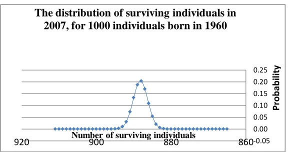
The distribution of surviving individuals in 2007 is calculated via the following equation
(20).The probability for surviving individuals is -
∫
for:
1526
We program the solution defined by the integral in equation (20) with its characteristics in (21)
via the Wolfram Mathematica software. The Mathematica code is provided in appendix B.
Table C.1 in appendix C reports the distribution of surviving individuals in 2007. The
distribution of surviving individuals in 2007 is also described in figure 1.
We can also forecast the estimated distribution of future survivors in any period in the future.
For example, we can forecast the distribution of survivors in 2015 for the same group of
individuals born in 1960. Let us go back to the SSA mortality tables which reports mortality rates
only until the year 2007. The cohort born in 1960 was 47 years old in 2007. However, we can use
the mortality rates data collected by the statistical agencies for 2007 for people at ages 48, 49, 50,
51, 52, 53, 54 and 55, and attribute them to the cohort born in 1960 and use it as estimation for the
2008, 2009, 2010, 2011, 2012, 2013, 2014, 2015 mortality probabilities, respectively. For example,
the mortality rate for the cohort at the age of 48 in 2007 is 0.004603. Thus, we can estimate the
forecasted 2008 mortality probability for the cohort born in 1960 as 0.004603 and thus we can
estimate the forecasted survival probability (that equals 1 minus the forecasted mortality
probability) as 0.995397. We continue to make these estimations until we reach the 2015 mortality
probability forecast. These forecasts are presented in table D.1 in appendix D.
Figure-1.
We showed before that for 1000 people born in 1960, the calculated probability of surviving
until 2006 (included) was 0.89195 and thus the expected number of survivors in 2006 was 891.947.
We can now calculate the probability of individuals born in 1960 to survive until 2014 (included)
by multiplying the calculated probability of surviving until 2006 by the probability of surviving
2007 (given in the SSA table as well as in table D.1) and by the forecasted probabilities of
surviving 2008-2014 (included), as reported in table D.1.
The estimated probability to survive until 2014 (included) is 0.85147 and thus the expected
number of survivors in 2014 is 851.471 (out of the original 1000 individuals born in 1960). Using
our technique and the forecasted survival probability for 2015 (which is 0.99203 – as reported in
table D.1), we can calculate the expected distribution of future survivors in 2015. The forecasted
distribution of future surviving individuals in 2015 is again calculated via equation (20), for:
-0.05 0.00 0.05 0.10 0.15 0.20 0.25
860 880
900 920
P
rob
ab
ili
ty
Number of surviving individuals
1527
( )
The forecasted distribution of the future survivors in 2015 is described in figure 2.
Figure-2.
3. RESULTS AND DISCUSSION
In most counties, the statistical authorities collect data on the number of deaths in each age
group. That enables the calculation of life expectancy as well as the calculation of death and
survival probabilities for each age group. However, many institutions (e.g., pension funds, geriatric
institutions and the medical authorities in general) would benefit from estimating the future
distribution of survivors as well.
In this paper, we develop a tool that can be used to estimate the future distribution of survivors
for each cohort. Such a distribution defines the probability for the number of survivors at a given
future time. Assuming individuals were born in period 0, and assuming that their probability to
survive time t is defined as
p
t, we can refer to the survival distribution at time t as a Bernoullidistribution. In the Bernoulli distribution, each agent faces a "successful trial" with probability
p
t(survival) and a failure with the probability
1
p
t(death). Using the Newton Binomial formula wecan calculate the probability that individuals will survive at any time T>t. As , the
binomial distribution function is expressed in terms of the standard normal distribution function.
Estimating the probability of surviving individuals in time T via the continuous normal
distribution solution requires a multiple-integral calculation. Alternatively, we suggest a compact
model in which the average expected number of individuals in time T-1, , is estimated by
multiplying the probability to survive from time 0 until time T-1 by the initial number of
individuals in time 0, . That allows us to express the probability of surviving individuals in
time T via a single integral over the density distribution function of the normal distribution, with
the integral boundaries of and .
For example, our tool enables us to calculate the whole distribution of surviving probabilities
in 2007. Using the mortality rates tables published by the SSA, we can calculate the probability of
-0.20 0.00 0.20
800 820
840 860
880
P
rob
ab
ili
ty
Number of surviving individuals
The forecasted distribution of surviving individuals in 2015, for 1000 individuals
1528
individuals born in 1960 to survive until 2006 (included). The probability of individuals born in
1960 to survive until 2006 (included) is 0.89195. Thus, among every 1000 individuals born in
1960, 891.947 will survive till the end of 2006, on average. We can also tell that, on average, out of
the 1000 original individuals, about 888 of them will survive till the end of 2007. But, there might
be a given probability that the realized number of survivals will be much larger or much lower than
the expected number. Thus, relying solely or mainly on the expected value of survivals, many
institutions such as pension funds, geriatric institutions and the medical authorities in general, may
end up extremely unbalanced. If such a company could estimate the distribution of the expected
future number of deaths for each cohort, it could expand its forecasting tools and thus reduce its
operational risks by using the confidence interval of the expected number of deaths instead of
solely using the expected value.
We can also forecast the estimated distribution of future survivors in any period in the future.
For example, we can forecast the distribution of survivors in 2015 for the same group of
individuals born in 1960. Naturally, the SSA mortality tables do not go into the future. However,
we can apply the current mortality rates data and use it as an estimate for the future mortality
probabilities for the cohort born in 1960.
Continuing our example, the estimated probability for the cohort born in 1960 to survive until
2014 (included) is 0.85147 and thus the expected number of survivors in 2014 is 851.471 (out of
the original 1000 individuals born in 1960). Using our technique and the forecasted survival
probability for 2015 (0.99203), we can calculate the expected forecasted distribution of future
survivors in 2015.
Thus, our paper contributes not only to the literature on the projection of mortality rates, but it
also has significant practical implications because it enables the authorities, as well as other
relevant institutions, to be better prepared for the upcoming future and to better handle unexpected
changes associated with it.
REFERENCES
Alderson, M. and F. Ashwood, 1985. Projection of mortality rates for the elderly. Population Trends, 42: 22–
29.
Biffis, E., 2005. Affine processes for dynamic mortality and actuarial valuations. Insurance. Mathematics and
Economics, 37: 443–468.
Booth, H. and L. Tickle, 2008. Mortality modelling and forecasting: A review of methods. Annals of Actuarial
Science, 3: 3–43.
Brouhns, N., M. Denuit and J.K. Vermunt, 2002. A poisson log-bilinear regression approach to the
construction of projected life tables. Insurance Mathematics and Economics, 31: 373–393.
Cairns, A.J.G., D. Blake, K. Dowd, G.D. Coughlan, D. Epstein, A. Ong and I. Balevich, 2009. A quantitative
comparison of stochastic mortality models using data from England & wales and the United States.
1529 Dahl, M., 2004. Stochastic mortality in life insurance: Market reserves and mortality-linked insurance
contracts. Insurance Mathematics and Economics, 35: 113–136.
Lee, R.D. and L.R. Carter, 1992. Modeling and forecasting U.S. Mortality. Journal of the American Statistical
Association, 87: 659–675.
Milevsky, M.A. and S.D. Promislow, 2001. Mortality derivatives and the option to annuitise. Insurance
Mathematics and Economics, 29: 299–318.
Olshansky, S.J., 1988. On forecasting mortality. The Milbank Quarterly, 66(3): 482–530.
Pollard, J.H., 1987. Projection of age-specific mortality rates. Population Bulletin of the United Nations, 21–
22: 55–69.
Renshaw, A.E. and S. Haberman, 2006. A cohort-based extension to the lee-carter model for mortality
reduction factors. Insurance Mathematics and Economics, 38: 556–570.
Schrager, D.F., 2006. Affine stochastic mortality insurance. Mathematics and Economics, 38: 81–97.
Appendix-A: Table-A.1. SSA data: mortality and survival rates for individuals born in 1960, for each year between 1960 and 2007
Year Age at that year Mortality rates Survival rates 1960 0 0.02937 0.97063 1961 1 0.00174 0.99826 1962 2 0.00105 0.99895
. . . .
. . . .
2005 45 0.00375 0.99625 2006 46 0.00397 0.99603 2007 47 0.00421 0.99579
Appendix-B: The Mathematica code for the distribution of surviving individuals in 2007, for 1000 individuals born in 1960:
strm=OpenWrite ["…fill in the required output path…"]
num=1000
For[m=0,m<num,m++,Write[strm,Integrate[1/Sqrt[2*Pi*n*p*(1-p)]*Exp[-(x-n*p)^2/(2*n*p*(1-p))], {x, m-0.5, m+0.5},Assumptions {n=891.947,p=0.99579}]]]
Appendix-C: Table-C.1. The distribution of surviving individuals in 2007, for 1000 individuals born in 1960.
Number of surviving individuals Probability
873 0.00000000000000
874 0.00000000000000
875 0.00000000002557
876 0.00000000071469
877 0.00000001534577
878 0.00000025319193
879 0.00000321078768
880 0.00003130266064
881 0.00023467355658
… …
… …
895 0.00047421435433
1530
896 0.00006996033194
897 0.00000793746239
898 0.00000069240502
899 0.00000004642806
900 0.00000000239241
901 0.00000000009471
902 0.00000000000000
903 0.00000000000000
Appendix-D: Table-D.1. Forecasted mortality and survival probabilities for the cohort born in 1960.
The cohort born at the year
Age at the year
2007 Mortality rates Survival rates
An estimation for the mortality
and survival probabilities for the cohort born in 1960 for the year
1959 48 0.004603 0.995397 2008
1958 49 0.005037 0.994963 2009
1957 50 0.005512 0.994488 2010
1956 51 0.006008 0.993992 2011
1955 52 0.006500 0.993500 2012
1954 53 0.006977 0.993023 2013
1953 54 0.007456 0.992544 2014