Pairwise FastText Classifier for Entity Disambiguation

Pairwise FastText Classifier for Entity Disambiguation

Cheng Yu

, Bing Chu

, Rohit Ram

, James

Aichinger

, Lizhen Qu

, Hanna Suominen

a

_{Project Cleopatra, Canberra, Australia}

_{The Australian National University}

c

_{DATA 61, Australia}

[email protected]

{u5470909,u5568718,u5016706,

Hanna.Suominen}@anu.edu.au

[email protected]

Abstract

For the Australasian Language Technology Association (ALTA) 2016 Shared Task, we devised Pairwise FastText Classifier (PFC), an efficient embedding-based text classifier, and used it for entity disambiguation. Com-pared with a few baseline algorithms, PFC achieved a higher F1 score at 0.72 (under the team name BCJR). To generalise the model, we also created a method to bootstrap the training set deterministically without human labelling and at no financial cost. By releasing PFC and the dataset augmentation software to the public1, we hope to invite more collabora-tion.

1

Introduction

The goal of the ALTA 2016 Shared Task was to disambiguate two person or organisation entities (Chisholm et al., 2016). The real-world motiva-tion for the Task includes gathering informamotiva-tion about potential clients, and law enforcement.

We designed a Pairwise FastText Classifier

(PFC) to disambiguate the entities (Chisholm et al., 2016). The major source of inspiration for PFC came from FastText 2 _{algorithm which}

achieved quick and accurate text classification (Joulin et al., 2016). We also devised a method to augment our training examples deterministically, and released all source code to the public.

The rest of the paper will start with PFC and a mixture model based on PFC, and proceeds to pre-sent our solution to augment the labelled dataset

1 _{All source code can be downloaded from:}

https://github.com/projectcleopatra/PFC

deterministically. Then we will evaluate PFC’s performance against a few baseline methods, in-cluding SVC3 _{with hand-crafted text features.}

Fi-nally, we will discuss ways to improve disambig-uation performance using PFC.

2

Pairwise Fast-Text Classifier (PFC)

Our Pairwise FastText Classifier is inspired by the FastText. Thus this section starts with a brief description of FastText, and proceeds to demon-strate PFC.

2.1 FastText

FastText maps each vocabulary to a real-valued vector, with unknown words having a special vo-cabulary ID. A document can be represented as the average of all these vectors. Then FastText

will train a maximum entropy multi-class classi-fier on the vectors and the output labels. Fast Text has been shown to train quickly and achieve pre-diction performance comparable to Recurrent Neural Network embedding model for text classi-fication (Joulin et al., 2016).

2.2 PFC

PFC is similar to FastText except that PFC takes two inputs in the form of a list of vocabulary IDs, because disambiguation requires two URL inputs. We specify that each of them is passed into the same embedding matrix. If each entity is repre-sented by a d dimensional vector, then we can concatenate them, and represent the two entities

2 _{The original paper of FastText used the typography} fastText

by a 2d dimensional vector. Then we train a max-imum entropy classifier based on the concatenated vector. The diagram of the model is in Figure 1.

Figure 1: PFC model. W1 and W2 are trainable weights.

2.3 The PFC Mixture Model

The previous section introduces word-embed-ding-based PFC. In order to improve disambigua-tion performance, we built a mixture model based on various PFC sub-models: Besides word-em-bedding-based PFC, we also trained character-embedding-based PFC, which includes one uni-character PFC, and one bi-uni-character PFC. In the following subsections, we will first briefly explain character-embedding-based PFC, and then show the Mixture model.

2.3.1 Character-Embedding-Based PFCs

Character-embedding-based PFC models typi-cally have fewer parameters than word-embed-ding-based PFC, and thus reducing the probability of overfitting.

Uni-character embedding maps each character in the URL and search engine snippet into a 13-dimensional vector, take the average of an input document, concatenate the two documents, and then train a maximum entropy classification on top of the concatenated vectors.

Bi-character embedding model has a moving window of two characters and mapped every such two characters into a 16-dimensional vector.

Our implementation of the character-embed-ding based PFC model includes only lowercase English letters and space. After converting all let-ters to lowercase, other characlet-ters are simply skipped and ignored.

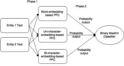
2.3.2 Mixing PFC Sub-models

The mixture model has two phases. In phase one, we train each sub-model independently. In phase 2, we train a simple binary classifier based on the probability output of each individual PFC. The di-agram of the PFC mixture model is shown in Fig-ure 2.

4 _{In the Shared Task, if a pair of URL entities refer to}

differ-ent persons or organisations, the pair belongs to the negative

Figure 2: The PFC Mixture Model.

3

Augmenting More Training Examples

Deterministically

Embedding-models tend to have a large number of parameters. Our word-embedding matrix has over 3700 rows, and thus it is natural to brain-storm ways to augment the training set to prevent overfitting.

We created a method to harvest additional training examples deterministically without the need for human labelling, and the data can be ac-quired at no additional cost.

3.1 Acquiring Training Examples for the Negative Class4

To acquire URL pairs that refer to different peo-ple, we wrote a scraping bot that visits LinkedIn, and grabs hyperlinks in a section called “People that are similar to the person”, where LinkedIn recommends professionals that have similar to the current profile that we are browsing. LinkedIn re-stricts the number of profiles we can browse in a given month unless the user is a Premium user, so we upgraded our LinkedIn account for scraping purpose. We used the LinkedIn URLs provided to us in the training samples, and grabbed similar LinkedIn profiles, which ended up with about 850 profiles, with some of the LinkedIn URLs no longer up to date.

3.2 Acquiring Training Examples for the Positive Class

To acquire training examples of different social media profiles that belong to the same person, we used examples from about.me. About.me is a platform where people could create a personal page showing their professional portfolios and links to various social media sites. We wrote a scraping bot that visits about.me/discover, where the site showcases their users, and clicks open

each user, acquires their social media links, and randomly selects two as a training example. For example, for someone with 5 social media pro-files, including Facebook, Twitter, LinkedIn, Pin-terest, and Google+, the bot can generate (5, 2) = 10 training examples.

4

Experimental Setup

Using the training data provided by the Organ-iser and data acquired using the method men-tioned in Section 3, we evaluated the perfor-mance of our PFC and PFC Mixture against a few baseline models.

4.1 Datasets

The organiser prepared 200 labelled pairs of train-ing samples and 200 unlabelled test samples (Hachey, 2016). All baseline methods and PFC methods are trained using the original 200 URL pairs. The only exception is “PFC with augmented dataset”, which uses the method in the previous section to acquire 807 negative class URL pairs, and 891 positive class URL pairs.

4.2 Pre-Processing

Text content for the PFC comes from the search engine snippet file provided by the Organiser and text scraped from the URLs provided by the train-ing examples. Unknown words in the test set are represented by a special symbol.

4.3 Baselines

The reason we choose a few baseline models is that there is no gold-standard baseline model for URL entity disambiguation. Baseline models are explained as followed.

Word-Embedding with Pre-Trained Vec-tors: The training corpus Google comes from News Articles (Mikolov et al., 2013). For each URL entity, we calculated the mean vector of the search result snippet text by using pre-trained word embedding vectors from Google. Unknown words were ignored. Then we concatenated the vectors and trained a maximum entropy classifier on top of it.

SVC with Hand-Selected Text Features: Our Support Vector Classifier is built on top of hand-selected text features. For each pair of URLs, we

5 _{F1 total is the simple average of F1 Public (calculated}

from half of half of the test data) and F1 Private (from the second half of the data)

manually selected the following text features. Ex-planation of these features is available in Appen-dix-A.

LSTM Word-Embedding: We passed each document token sequentially using word embed-ding into an LSTM layer with 50 LSTM units (Brownlee, 2016) (Goodfellow et al., 2016), con-catenated the two output vectors, and trained a maximum entropy classifier on top of it. To re-duce overfitting, we added dropout layers with the dropout parameter set to 0.2 (Zaremba, Sutskever, & Vinyals, 2014).

Neural Tensor Network: Inspired by Socher et al., by passing a pair of documents represented in vector form into a tensor, we built a relationship classifier based on the architecture in the paper (Socher et al., 2013). Document vectors are calcu-lated from pre-trained Google embedding word vectors.

5

Results and Discussion

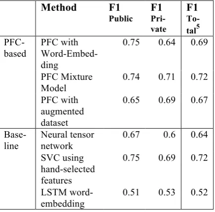
The experimental results from the setup is sum-marised in the table.

Method F1

Public F1 Pri-vate

F1 To-tal5

PFC-based

PFC with Word-Embed-ding

0.75 0.64 0.69

PFC Mixture Model

0.74 0.71 0.72

PFC with augmented dataset

0.65 0.69 0.67

Base-line

Neural tensor network

0.67 0.6 0.64

SVC using hand-selected features

0.75 0.69 0.72

LSTM word-embedding

0.51 0.53 0.52

Table 1: Result comparison.

5.1 Issues with Augmented Dataset

with approximately equal number in each cate-gory. Whether adding more training data can im-prove disambiguation performance remains to be experimented.

5.2 Improve PFC

The performance of the PFC might improve if we use a similarity scoring function 𝑠 𝑣_#, 𝑣_% =

5.3 Compare PFC with Baseline SVC

In our experiments, the PFC mixture model achieves the best performance, comparable to SVC with hand-selected features. Uni-character model by itself tends to under fit because the train-ing data themselves cannot be separated by the model alone. PFC is robust because allows text features to be learnt automatically.

6

Conclusion

We introduced Pairwise FastText Classifier to disambiguate URL entities. It uses embedding-based vector representation for text, can be trained quickly, and performs better than most of the al-ternative baseline models in our experiments. PFC has the potential to generalise towards a wide range of disambiguation tasks. In order to gener-alise the application of the model, we created a method to deterministically harvest more training examples, which does not require manual label-ling. By releasing all of them to the public, we hope for the continual advancement in the field of disambiguation, which could be applied to iden-tity verification, anti-terrorism, and online general knowledge-base creation.

Appendix A

Appendix A includes manually selected text features for the SVC baseline model.

A.1 URL Features

ID Feature Name Description

1 Country code dif-ference

If one URL has “au” and another one has “uk”, then the value is 1, otherwise 0. 2 Edit distance

be-tween the two URLs

Simply the Levenshtein distance between the string tokens of the two URLs (Jurafsky & Martin, 2007).

Below are a list of URL features specific to one URL.

3 isEducation(url_a) If the first URL con-tains domain names such as “.ac.uk” or “.edu”, then the value is 1. Otherwise 0.

4 isEntertain-ment(url_a)

If the url includes imdb, allmusic, artnet, mtv.com, or band, it re-turns 1. Otherwise 0. 5

isProfes-sional(url_a)

If the url contains linkedin.com or searchgate.com, it re-turns 1. Otherwise 0. 6

isNonProfitOr-Gov(url_a)

If the url contains “.org” or “.gov”, then it returns 1.

7 isSportsStar(url_a) If the url contains “espn”, “ufc.com”, or “sports”, then the fea-ture is 1. Otherwise 0. 8 -

12

Features for url_b Analogous to Feature 3 - 7

A.2 Title Features ID Feature

Due to the differences of length between different titles, only the first part of the titles is pre-served for calculating the Le-venshtein distance. This feature is chosen because the first part of the title usually contains the first and last name of the person or the name of the company. 14 Cosine

distance of the em-bedded matrices

The vector representation of the text is same as FastText except that the embedding matrix is pre-trained from Google. Any token not trained by Google will be ignored (Weston, Chopra, & Bordes, 2015).

A.3 Snippet Features

This refers to features made from fields “ASnip-pet” and “BSnip“ASnip-pet” of the search result file pro-vided by the Organiser.

ID Feature Name Description

15 Word Mover Distance be-tween the nouns and named entities between “ASnippet” and “BSnip-pet” (Pele & Werman, A linear time histogram metric for improved sift

matching, 2008) (Pele & Werman, Fast and robust earth mover’s distances, 2009).

16 Word Mover Distance be-tween the nouns and named entities between “ASnippet” and “BSnip-pet”

Using the pre-trained Stanford GloVe vectors (Pennington et al., 2014).

Reference

Brownlee, J. (2016, July 26). Sequence Classification with LSTM Recurrent Neural Networks in Python with Keras. Retrieved from Machine Learning Mastery:

http://machinelearningmastery.com/sequence

-classification-lstm-recurrent-neural-networks-python-keras/

Chisholm, A., Hachey, B., & Molla, D. (2016). Overview of the 2016 ALTA Shared Task: Cross-KB Coreference. Proceedings of the Australasian Language Technology Association Workshop 2016.

Chisholm, A., Radford, W., & Hachey, B. (2016). Discovering Entity Knowledge Bases on the Web. Proceedings of the 5th Workshop on Automated Knowledge Base Construction

Goodfellow, I., Bengio, Y., & Courville, A. (2016). Deep Learning, pages 373 - 420.

Hachey, B. (2016). How was the data obtained? - ALTA 2016. Retrieved from Kaggle: https://inclass.kaggle.com/c/alta-2016- challenge/forums/t/23480/how-was-the-data-obtained

Joulin, A., Grave, E., Bojanowski, P., & Mikolov, T. (2016). Bag of Tricks for Efficient Text Classification. arXiv preprint

arXiv:1607.01759.

Jurafsky, D., & Martin, J. H. (2007). Speech and Language Processing, 3rd edition [Draft]. Chapter 2.

Mikolov, T., Chen, K., Corrado, G., & Dean, J. (2013). Efficient Estimation of Word Representations in Vector Space. arXiv preprint arXiv:1301.3781.

Pele, O., & Werman, M. (2008). A linear time histogram metric for improved sift matching. Computer Vision--ECCV 2008.

Pele, O., & Werman, M. (2009). Fast and robust earth mover’s distances. 2009 IEEE 12th

International Conference on Computer Vision.

Pennington, J., Socher, R., & Manning, C. D. (2014). GloVe: Global Vectors for Word

Representation. Empirical Methods in Natural Language Processing, pages 1532 – 1543.

Socher, R., Chen, D., Manning, C., & Ng, A. (2013). Completion, Reasoning With Neural Tensor Networks for Knowledge Base. In Advances in Neural Information Processing Systems, 2013a.

Weston, J., Chopra, S., & Bordes, A. (2015). Memory Networks. arXiv:1410.3916.