DOI: 10.1534/genetics.108.092221
A Genome-Scan Method to Identify Selected Loci Appropriate for Both
Dominant and Codominant Markers: A Bayesian Perspective
Matthieu Foll
1and Oscar Gaggiotti
Laboratoire d’Ecologie Alpine (LECA), CNRS UMR 5553, 38041 Grenoble Cedex 09, France
Manuscript received June 3, 2008 Accepted for publication July 23, 2008
ABSTRACT
Identifying loci under natural selection from genomic surveys is of great interest in different research areas. Commonly used methods to separate neutral effects from adaptive effects are based on locus-specific population differentiation coefficients to identify outliers. Here we extend such an approach to estimate directly the probability that each locus is subject to selection using a Bayesian method. We also extend it to allow the use of dominant markers like AFLPs. It has been shown that this model is robust to complex demographic scenarios for neutral genetic differentiation. Here we show that the inclusion of isolated populations that underwent a strong bottleneck can lead to a high rate of false positives. Nevertheless, we demonstrate that it is possible to avoid them by carefully choosing the populations that should be included in the analysis. We analyze two previously published data sets: a human data set of codominant markers and aLittorina saxatilisdata set of dominant markers. We also perform a detailed sensitivity study to compare the power of the method using amplified fragment length polymorphism (AFLP), SNP, and microsatellite markers. The method has been implemented in a new software available at our website (http://www-leca.ujf-grenoble.fr/logiciels.htm).
O
NE of the main challenges of modern biology is to dissect and understand the molecular basis for naturally occurring genetic variation. Recent advances in the fields of computational biology and molecular biology techniques have led to the emerging field of ‘‘population genomics,’’ whose main objective is to char-acterize the parts of the genome subject to natural se-lection. This new discipline has important applications in many domains such as medical genetics and the improvement of agricultural crops and breeds. Addi-tionally, ignoring the effect of natural selection in evolutionary studies can lead to wrong estimates of the demographic history of species. Therefore, sepa-rating the effect of neutral drift and adaptive genetic differentiation is a necessary preliminary step in most analyses of genomewide data sets, and this distinction can also help us to understand speciation processes.A wide variety of methods have been developed to identify regions of the genome that have been subject to natural selection (see Nielsen et al. 2005, for a
re-view). Among them, we can distinguish those based on comparative data (taken from different species) that can detect old signatures of selection and those using population genomics data that allow the detection of more recent ones. This latter family of methods has became very popular in the last decade and has been
applied to many nonmodel species (see Wildinget al.
2001, for example).
Many of the existing methods for detecting recent selection from population genomics data are based on an idea first introduced by Lewontinand Krakauer(1973)
(see, for example, Bowcocket al.1991; Beaumontand
Nichols 1996; Vitalis et al. 2001; Beaumont and
Balding 2004). The basic rationale is that loci
influ-enced by directional (also called adaptive or positive) selection will show a larger genetic differentiation than neutral loci, and loci that have been subject to balancing (also called negative or purifying) selection will show a lower genetic differentiation. Thus, the methods gen-erally consist of identifying loci that present FST
co-efficients that are ‘‘significantly’’ different from those expected under the neutral theory (they are called outlier loci).
Lewontinand Krakauer’s (1973) method has raised
many criticisms (see Beaumont2005, for more details
about them) and finally fell out of use. More recently, Bowcock et al. (1991) and Beaumont and Balding
(2004) showed that problems of a purely statistical nature can be easily solved. In particular, the problem related to the correlation of allele frequencies among demes can be overcome by adopting a Bayesian ap-proach that implements the multinomial-Dirichlet likelihood, which arises in a wide variety of neutral pop-ulation genetic models (see Balding2003). One of the
scenarios covered consists of an island model (Wright
1931) in which subpopulation allele frequencies are
1Corresponding author:Computational and Molecular Population Ge-netics Lab, Zoology Institute, Baltzerstrasse 6, 3012 Bern, Switzerland. E-mail: [email protected]
correlated through a common migrant gene pool from which they differ in varying degrees. The difference in allele frequency between this common gene pool and each subpopulation is measured by a subpopulation-specificFST. Therefore, this formulation can consider
more realistic ecological scenarios where the effective size and the immigration rate may differ among sub-populations. Additionally, a previous study (Foll and
Gaggiotti 2006) has shown that statistical methods
based on this approach are robust to deviations from the underlying demographic model.
As opposed to the multinomial-Dirichlet approach, most existing methods to detect outlier loci are based on simpler demographic models. More precisely, Beaumontand Nichols(1996) used a model with an
infinite number of islands, all of which have equal sizes and exchange migrants at the same rate. A violation of this model can lead to a high false-positive rate and, in particular, it requires the consideration of a large number of subpopulations (Flint et al. 1999). The
mutation rate, the mutation model, and the demo-graphic history may also have a large effect on the distribution ofFST, especially if heterozygosities are high
(see the manual of the FDist2 program implementing this method). More recently, Vitaliset al.(2001)
pro-posed an alternative model to obtain the expected distribution ofFSTunder the neutral scenario. For this
purpose, they use coalescence simulations of pairs of haploid populations that do not exchange migrants and are of constant size, having diverged from an ancestral population that may have experienced a bottleneck before splitting. This method has the disadvantage of considering a model consisting of a single pair of populations and, therefore, the authors recommend to identify a locus as an outlier only if it is identified as such in all or most of the pairwise comparisons that include a particular population (Vitaliset al. 2001). The
prob-lem with this approach is that the pairs of populations analyzed are not independent and it is impossible to define rigorousP-values in this case. For this reason, this method is suitable to detect only extreme cases of natural selection. Both of the methods discussed above share an additional drawback: the expected distribution of FST is obtained by simulating a large number of
neutral data sets using as input parameters the estimates obtained from the real data set. The problem is that, ideally, input parameters should be based only on neutral markers, and, therefore, the presence of se-lected loci in the data set can lead to biases. Ad hoc
procedures can be used to reduce this problem but they are fairly subjective.
Instead of focusing onFST’s as a means of detecting
outliers, it is also possible to consider the heterozygosity or some other measure of genetic diversity. Schlotterer
(2002) and Kauer et al. (2003) proposed such an
approach that is suitable for microsatellites markers because it assumes a strict stepwise mutation model
(SMM). They follow Vitaliset al.(2001) and consider
statistics based on pairs of populations. More precisely, they proposed to use the ratioRof the genetic diversity u ¼4Nemof two populations, where Neis the effective
population size andmis the mutation rate.uis estimated either from the varianceVin repeat number of micro-satellites or from the expected heterozygosityH, leading respectively to the so-called ln RVand ln RH statistics. Instead of using coalescence simulations to generate the expected distribution under neutrality, Schlotterer
(2002) uses the empirical distribution of ln RVand ln
RHstatistics and identifies as outliers those loci that fall outside the 95% confidence interval, under the assump-tion that the distribuassump-tion is normal. The drawback of this method is that the use of an empirical distribution necessarily leads to a high false-positive rate. In addition, this approach is also primarily designed for pairs of populations and is suitable to detect only extreme cases of natural selection.
As mentioned before, the more recent method pro-posed by Beaumontand Balding(2004) is based on the
multinomial-Dirichlet likelihood and considers thatFST
values integrate effects that are specific to each popula-tion and to each locus. Thus, a locus is deemed to be under selection if the equal-tailed 100(1 –P)% posterior interval for its locus-specific effect excludes zero. Al-though this method avoids all the above-described problems it still has the drawback of not providing a rigorous way of testing the hypothesis that a locus is subject to selection. To address this problem, Riebler
et al.(2008) extended the method by introducing the
use of a Bernoulli-distributed auxiliary variable, di, to indicate whether or not a locus is subject to selection. Then, they classify a locusias being under selection if the posterior probabilityP(di¼1jdata) is larger than a threshold value that is set by means of a simulation study. Although this may represent an improvement over the original method, it still requires the use of a simulation study. The authors propose to use a cutoff value of 0.17 on the basis of their simulations but it is unlikely that this value will be appropriate for all data sets.
Here we propose a different and more rigorous approach to develop a test for selection. More specifi-cally, we directly estimate the posterior probability of a given locus being under the effect of selection by defining two alternative models, one that includes the effect of selection and another that excludes it; we then estimate their respective posterior probabilities using a reversible-jump MCMC approach. Additionally, we ad-dress a common limitation of all the methods described above (except that of Beaumont and Nichols1996)
that can be used only with codominant markers. More specifically, we generalize the method of Beaumontand
Balding(2004) by making it applicable to dominant
compare the power of the method using AFLP, SNP, and microsatellite markers.
Another issue that has not been considered in the past is the extent to which the demographic history of species and differences in mutation rates among loci can bias the detection of selection using genome scans. To address this issue we present the results of a simulation study that considers the effect of spatial expansions such as that undergone by humans. Addi-tionally, we study the effect of not discriminating be-tween di-, tri-, and tetranucleotide microsatellites when carrying out genome scans. Finally, we illustrate how the method can be applied to study particular cases by analyzing published data sets on humans and periwinkles.
METHODS
Bayesian model for estimation of locus–population-specific FSTcoefficients:The model for genetic differ-entiation used is based on ideas first introduced by Baldingand Nichols(1995) and that Beaumontand
Balding(2004) later used to detect loci under natural
selection. Strictly speaking, the approach applies to an island model (Wright1931) but it has also been used
to describe a fission model (Falush et al. 2003). For
the sake of simplicity we describe the details of our approach using the terminology of this latter model. We consider a collection of Jsubpopulations that evolved in isolation after splitting from an ancestral population. The derived subpopulations may have been subject to different amounts of genetic drift and, therefore, their allele frequencies will show different degrees of differ-entiation from the ancestral allele frequency. We con-sider a set ofIloci and letKibe the number of alleles at theith locus. The extent of differentiation at locusi
between subpopulationjand the ancestral population is measured byFSTij and is the result of its demographic
history. Letpi¼{pik} denote the allele frequencies of the ancestral population at locusi, wherepikis the frequency of the allele k at locus iðPkpik¼1Þ. We use p ¼{pi} to denote the entire set of allele frequencies of the ancestral population and fpij ¼ fpfijkg to denote the
current allele frequencies at locusifor subpopulation
j. Under these assumptions, the allele frequencies at locusiin subpopulationjfollow a Dirichlet distribution with parametersuijpi,
f
pij Dirðuijpi1;. . .;uijpiKiÞ; ð1Þ
where uij¼1=F ij
ST1. The parameters F
ij
ST are very
closely related to Wright’s (1951)FST parameter and
are interpreted as measures of the shared ancestry within each of the subpopulations (see Balding2003,
for a more detailed explanation). The full prior dis-tribution can be obtained by multiplying across loci and populations:
pðp˜jp;uÞ ¼Y I
i¼1
YJ
j¼1
pðfpijjpi;uijÞ: ð2Þ
Hierarchical model for locus- and population-specific effects: The amount of data available to es-timate all locus–population-specific FSTcoefficients is
reduced and this leads to inaccurate estimates, espe-cially for loci with a small number of different alleles. As an alternative, Balding et al. (1996) proposed to
de-compose locus–population-specificFSTcoefficients into
a population-specific component,bj, shared by all loci and a locus-specific component, ai, shared by all pop-ulations. We use the model proposed by Beaumontand
Balding(2004) that is based on the following equation:
log F
ij
ST 1FSTij
!
¼log 1
uij
¼ai1bj: ð3Þ
The advantage of this formulation is that instead of estimatingIJ FSTij coefficients, we have to estimate only
theIparametersaiand theJparametersbj. In the case of absence of natural selection, all ai coefficients are excluded, and the above model is equivalent to the one used by Folland Gaggiotti(2006), where the termbjis
replaced by a generalized linear model. Note that with this formulation,FSTij and equivalentlyuijare no longer model parameters that need to be estimated because they are replaced by ai and bj parameters. In what follows we useuijfor the sake of simplicity but note that it can be replaced directly byuij¼exp(– (ai1bj)).
Beaumontand Balding(2004) originally proposed
to include a locus–population parameter gij in their formulation. However, they noted that the posterior probability for this parameter was very similar to the prior used. This indicates that there is not enough information to estimate it and, therefore, we chose here to exclude thegij’s from the model.
Estimating the probability that a locus is influenced by selection: To infer which loci are influenced by selection we focus on the posterior distribution ofai: a positive value suggests that the locus i is subject to directional selection, whereas a negative value suggests balancing selection. However, before deciding on the type of selection we need to decide whether or not there is selection at all. In their original formulation, Beaumontand Balding(2004) focused on the
probabil-ity of each one of these models. At each iteration of the MCMC algorithm, we propose to remove ai from the model if it is currently present or to add it if it is not included; this is done separately for each locusi. For example, if we propose to addaito the vectoraof locus effects, we draw a proposed value from a distributionq. Then we accept to add this locus in the model with probability min(1,A), where
A¼ pðp˜jp;a;bÞpðaiÞ
pðp˜jp;awithai ¼0;bÞqðaiÞ:
Because we only have two models and we choose them uniformly, the ratio of prior model probability simplifies to one. The Jacobian is one because of the canonical jump function used. To consider the reverse move, we simply accept the move deleting ai with probability min(1, 1/A). The proposal distribution qis a normal distribution with its mean and variance pilot tuned to improve convergence (see below).
With this method, we have posterior estimates of the probability that a locus is subject to selection: P(ai included) corresponds toP(ai6¼0). This probability is estimated directly from the output of the MCMC by simply by counting the number of timesaiis included in the model.
Estimating allele frequencies: Beaumont and
Balding’s (2004) original formulation considered
co-dominant markers; here we extend it to co-dominant ones. Note that we have to estimate the allele frequency of each subpopulation and that of the ancestral popula-tion because they are unknowns. Thus, we present two different formulations depending of the type of marker used: codominant (like microsatellites or SNPs) and dominant (like RFLPs or AFLPs).
Codominant markers:The data consist of allele counts
obtained from samples of sizenij. We useaijkto denote the number of alleles k observed at locus i in the sample from subpopulationj. Thus,nij ¼
P
kaijk. The full data set can be presented as a matrix N¼ faijg, where aij¼ faij1;aij2; . . .;aijKig is the allele count at
locus i for subpopulation j. The observed allele frequencies, aij, can be considered as sampled from the true alleles frequenciespfij and, therefore, can be
described by the multinomial distribution (Holsinger
1999):
aij Multinomialfnij;pfij1;pfij2;. . .;pgijKig: ð4Þ
In principle, we could use as likelihood the multino-mial distribution (Equation 4) and consider Equation 1 as a Bayesian prior. However, in our case, we can calculate exactly the marginal distribution ofaijbecause the Dirichlet distribution is the conjugate prior of the multinomial. This allows us to eliminate the nuisance parameters fpij that are not of immediate interest but
are needed by the model. Thus, we obtain the multino-mial-Dirichlet distribution:
Pðaijjpi;ai;bjÞ ¼
nij!GðuijÞ
Gðnij1uijÞ
YKi
k¼1
Gðaijk1uijpikÞ
aijk!GðuijpikÞ
:
The likelihood is obtained by multiplying across all loci and populations:
Lðp;a;bÞ ¼Y
I
i¼1
YJ
j¼1
Pðaijjpi;ai;bjÞ: ð5Þ
Since the allele frequencies in the ancestral population are unknown, we have to estimate them by introducing a noninformative Dirichlet prior,pi Dirð1;. . .;1Þ, into our Bayesian model.
Dominant markers:Estimating allele frequencies from
dominant markers is more difficult because of the inability to distinguish heterozygous individuals from those that are homozygous for the dominant allele. Nevertheless, they have became very popular in the last decade, mostly due to the development of the AFLP marker, an inexpensive and easy way of obtaining large number of genetic markers from a wide variety of organisms (Bensch and Akesson 2005; Meudt and
Clarke2007). For each individual the information is
‘‘band presence’’ or ‘‘band absence,’’ which can be viewed as a phenotype. One possible solution is to suppose Hardy–Weinberg equilibrium to estimate allele frequencies but this imposes the strong hypothesis of no inbreeding. Holsingeret al.(2002) first proposed a
general method that includes the estimation of the inbreeding coefficientFIS.
In the context of dominant markers, the data N consist of the sample counts of observed phenotypes instead of allele counts. Let n[A1],ij and n[A2],ij be the observed number of phenotypes [A1] and [A2] at locus
i for population j. The full data set is presented as a matrixN¼ fn½A1;ij;n½A2;ijgand the sample size at locus
i for population j is nij ¼ n[A1],ij 1 n[A2],ij. We can
consider that the number of phenotypesn[A1],ijfollows a binomial distribution with parametersg[A1],ijandnij, whereg[A1],ijis the unknown [A1] phenotype frequency at locusiin populationj:
n½A1;ij Binomialðg½A1;ij;nijÞ: ð6Þ
Lðp˜;FISÞ ¼
YI
i¼1
YJ
j¼1
Pðn½A1;ijjg½A1;ijÞ:
The phenotype frequency g[A1],ij can be linked to the corresponding frequency pij of allele A1 and the inbreeding coefficient FISj of population j using the
following equations:
g½A1;ij¼fpij2ð1FISjÞ1F
j
ISfpij1ð1FISjÞ2fpijð1fpijÞ ð7Þ
g½A2;ij¼ ð1FISjÞð1fpijÞ21FISjð1fpijÞ ð8Þ
¼1g½A1;ij: ð9Þ
However, Foll et al. (2008) show that estimates
obtained from this model are strongly influenced by the ascertainment bias of AFLPs. They proposed an alterna-tive approximate Bayesian computation (ABC) approach that gives unbiased estimates of population-specificFST
and FIS coefficients. This solution leads to more
un-certainty on posterior distributions, which precludes the estimation of locus-specific ai’s. Additionally, the ABC algorithm cannot be used to estimate the posterior probability of each hypothesis of the formai¼0. Because here values of FIS are not of immediate interest, we
propose an intermediate solution: we do not estimateFIS
coefficients but we incorporate the full uncertainty on
FISby letting it move freely between 0 and 1 during the
MCMC process. This approach has also been proposed for the software Hickory, implementing the method of Holsingeret al.(2002), and is described in the online
manual (Holsingerand Lewis2002). Of course if some
other source of information suggests that inbreeding can be bounded within a narrower interval it is possible to restrict it to reduce uncertainty on parameter estimates. We use the prior on ancestral allele frequencies proposed
by Follet al.(2008):pi betaða;aÞ. The parametera
describes the shape of allele frequencies in the ancestral population (Wright1931) and is estimated using a
log-normal positive prior:a log Normalð0;1Þ.
Implementation: For codominant markers, the full Bayesian model represented by the directed acyclic graph (DAG) in Figure 1A is given by
pðp;a;bjNÞ}Lðp;a;bÞpðpÞpðaÞpðbÞ: ð10Þ
For dominant markers, the full Bayesian model represented by the DAG in Figure 1B is given by
pðp;FIS;p˜;a;b;ajNÞ}Lðp˜;FISÞpðp˜jp;a;bÞpðFISÞ
pðpjaÞpðaÞpðbÞpðaÞ:
ð11Þ
Following Beaumont and Balding (2004), for the
population effects bj, we used a Gaussian prior with mean 2 and standard deviation 1.8; for the locus effects,ai, we used a Gaussian prior with a zero mean and a standard deviation of 1. As explained above,FISj’s
are not estimated during the MCMC algorithm but are used to incorporate the uncertainty on inbreeding in the model with dominant markers.
The estimation of model parameters is carried out using a combination of MCMC and reversible-jump (RJ)MCMC (Green 1995) techniques that are
de-scribed in the supplemental information. We evaluated the convergence of the method using the diagnostic tests implemented in the R BOA package (Smith2005).
The tests indicated that a burn-in of 10,000 iterations was enough to attain convergence and it has been implemented as part of the pilot-tuning process (see below). We used a sample size of 10,000 and a thinning interval of 50 as suggested by an autocorrelation analysis. With these parameter values, the total length Figure1.—DAG of the models given in Equation 10 (A) and Equation 11 (B). The square node denotes known quan-tity (i.e., data) and circles represent parameters to be esti-mated. Lines between nodes represent direct stochastic relationships within the model. The variables within each node correspond to the different model parameters discussed in the text. N is the genetic data, that is, allele-frequency counts for codominant markers or phenotype-frequency counts for dominant data.p˜ andpare, respectively, the allele frequencies in each local population and in the ancestral pop-ulation. u is the vector of the genetic differentiation coeffi-cient for each local population. a and b are, respectively, the vectors of locus- and population-specific effects of the ge-netic differentiation. The vector u is represented within a dashed circle because it is not actually a parameter of the model: it can be calculated directly from Equation 3, but we represent it for a better understanding of the diagram.
of the chain was 500,000 iterations. The method has been implemented in a software written in C11. We provide a command line version for Linux and a version with a friendly user graphical interface for Microsoft Windows.
Proposal distributions have to be adjusted to have acceptance rates between 0.25 and 0.45. If we propose values in a very wide interval, most moves will be rejected because they will correspond to areas of low posterior probability. On the other hand, if we propose values very close to the current one, the move will be almost always accepted but the chain will take a long time to explore all the parameter space. These values are automatically tuned on the basis of short pilot runs: we run 2000 iterations, and for each parameter the proposal is adjusted to reduce or increase the acceptance rate. We make 10 such pilot runs before starting the sampling, which also play the role of a burn-in period. At the same time, we can choose the proposal distributionqfor the reversible jump. Brookset al.(2003) showed that the
best choice is to take qðaÞ to be the full conditional distribution ofain the saturated model. Because we do not know this distribution, we use the pilot run to get rough estimates of the meanmiand the variancevifor all aiunder the saturated model (in which all parametersai are included). Then we propose a new value foraifrom
N ðmi;viÞthat is generally close to the full conditional distribution.
SIMULATION STUDY
We investigated the performance of our method under different scenarios using a simulation study and also compared its performance with that of Beaumont
and Balding’s (2004) approach. This latter approach
has already been shown to perform better in various scenarios than the previous approaches based on the same idea (Beaumontand Balding2004).
Our first simulation approach uses the same statistical model assumed by our method (the inference model) and allows us to study the effect of three critical pa-rameters of the model in the identification of selection: the sample sizes, the number of populations, and the level of genetic differentiation. We also use this simula-tion scheme to compare the power of three different types of markers: AFLPs, SNPs, and microsatellites. The first marker is a dominant marker while the two others are codominant.
We also used a second simulation approach to in-vestigate the effect of departures from the demographic model assumed by our method. For this purpose we generated neutral marker data sets under a population expansion model that assumes a stepping-stone coloni-zation process (SPLATCHE, Currat et al.2004). This
allows us to investigate if the confounding effect of selection and demographic history can lead the method
to identify as selected loci that are in fact neutral (false-positive detection of selection).
Basic simulation design: Our initial simulation scheme assumes 1000 loci of which 100 are under directional selection and 100 are under balancing selection. Later on we also considered cases where only 100 loci are influenced by selection (50 balancing and 50 directional). We introduced selection usinga ¼2 and a ¼ 2 for directional and balancing selection, respectively. To have an idea of the strength of natural selection implied by these values, it is necessary to consider the extent to which a value ofFSTfor a neutral
marker (backgroundFST) is increased when a value of
2 is used foraiin Equation 3. Figure 2 shows the effect of aiwhen the backgroundFSTis 0.1. Additionally, Figure 2
in Beaumontand Balding(2004) showsFSTvalues for
three different selection coefficients (s¼0.02, 0.05, 0.1) and for the same backgroundFST. From these figures
it is possible to obtain Table 1, which relates the selection coefficient with the ai-values. Table 1 shows that anai¼2 is equivalent to ansslightly.0.05.
To investigate the performance of the method under different scenarios, we considered a default set of values for parameters that were common to both codominant and dominant markers and then changed values of one parameter at a time. This procedure led to 10 different data sets that are described in Table 2. The default values were six populations, a sample size of 30 Figure2.—Influence of thea-coefficient onFSTfor a back-groundFcST¼0:1. On the basis of Equation 3 we calculate the FSTcoefficient that a locus under selection with a given ai
would have. For this we first obtain the value of the popula-tion-specific effect for a chosen background FST from ˆb¼
logðFST=ð1FSTÞÞ and then obtain the corresponding value
under selection using FST¼expða1bˆÞ=ð11expða1bˆÞÞ.
For example, if an initially neutral marker exhibiting an
c
FST¼0:1 is subject to selection witha¼ 2, then we expect
that its FSTwill increase to 0.45 once a new equilibrium is
reached. Dashed lines connect theFSTvalues given in Table
individuals per population, and an FST coefficient
of 0.10.
In the particular case of AFLP markers we also need to consider the effect of inbreeding so we used a default value of 0.5 and two additional values (0 and 1; corresponding data sets are called Fis-0, Fis-0.5, and Fis-1 in Table 3) leading to a total of 12 different data sets. Additionally, we included in the simulation the ascertainment bias process observed for AFLP markers and described by Follet al.(2008). The bias we imposed
ensures that at least 2% of the total number of in-dividuals have a band and that at most 2% do not have a band. We used default parameters that we modified one by one to obtain the 12 data sets.
Allele frequencies in the ancestral population for both AFLPs and SNPs were generated from aU-shaped beta distribution with both parameters equal to 0.7. As Wright (1931) showed, at equilibrium, this implies
4Nm¼0.7, whereNis the effective population size and mis the mutation rate. In the case of microsatellites, we could simply use the noninformative Dirichlet prior with all parameters equal to 1 assumed by our inference model for multiallelic markers. However, Pritchard
and Feldman(1996) showed that the stepwise mutation
model describes better the mutation process of micro-satellites, and Graham et al. (2000) found that the
Dirichlet distribution is not appropriate in that case. In particular, simulating ancestral allele frequencies from their prior distribution would lead to a higher variability than what is generally observed in real data sets, and this would artificially increase the power of our method. To take into account this finding and at the same time evaluate the influence of a violation of the underlying infinite-alleles model assumption, we follow the ap-proach of Lockwood et al. (2001) to simulate allele
frequencies similar to those observed in real micro-satellites. They considered a maximum of seven differ-ent alleles and fixed the vector of allele frequencies in the ancestral population at each locus to (0.05, 0.1, 0.2, 0.3, 0.2, 0.1, 0.05). Although Moran(1975) showed that
no equilibrium distribution can be obtained under a stepwise mutation model, this provides a practical way
to simulate realistic microsatellite data sets. To allow variability in the ancestral population, we simulate the vector of allele frequencies at each locus from a Dirichlet distribution with parameters (10, 20, 40, 60, 40, 20, 10).
For some of the scenarios considered for AFLPs and SNPs, we observed a true-positive rate of 1 for micro-satellite data sets. Thus, we decided to enlarge the range of parameter values considered for this marker and instead of presenting results for data sets where all 200 loci under selection were correctly identified we simu-lated additional data sets corresponding to samples of lower quality. More specifically, we added simulations with four populations, FST ¼ 0.01, FST ¼ 0.03, 10
individuals in each population, jaj ¼ 0.5, jaj ¼ 1.0, and jaj ¼1.5 (respectively called Pop-4, 0.01, Fst-0.03, size-10, alpha-0.5, alpha-1.0, and alpha-1.5 in Table 5).
To decide whether or not a locus iis influenced by selection, we need to choose a cutoff value for the posterior probability P(ai 6¼0). All loci for which this posterior probability is larger than the cutoff value are considered as outliers. Ideally, one should choose a high value such as 0.95 or 0.99; however, if the purpose is to compare the performance of different types of markers, one needs to chose cutoff values that depend on the quality of the data set considered. For example, retain-ing only loci with a posterior probability .0.99 using microsatellites with a large sample size and many pop-ulations will lead to both a very low false-positive rate and a very high true-positive rate. By contrast, using the same cutoff value with the much less informative dominant markers will not allow us to detect many markers that are indeed under selection. For this rea-son, a pragmatic way to compare results between
TABLE 1
Equivalence betweenaiand selection coefficient
s FSTrange Mean a
0.02 [0.1; 0.4] 0.25 1.12
0.05 [0.2; 0.6] 0.4 1.8
0.1 [0.5; 0.8] 0.65 2.8
The relationship between the selection coefficients,s, and locus-specific effectsaifor a backgroundFSTof 0.1 is shown.
The second and third columns show theFST’s of the loci
un-der selection and were obtained from Figure 2 in Beaumont and Balding(2004). The fourth column shows thea-values for a givenFSTunder selection and is obtained from Figure 2.
TABLE 2
Simulation parameters
Name Populations FST Sample size
Pop-2 2 0.15 30
Pop-6a 6 0.15 30
Pop-10 10 0.15 30
Pop-20 20 0.15 30
Fst-0.05 6 0.05 30
Fst-0.10 6 0.1 30
Fst-0.15a 6 0.15 30
Fst-0.25 6 0.25 30
Size-15 6 0.15 15
Size-30a 6 0.15 30
Size-50 6 0.15 50
Size-100 6 0.15 100
Parameters used in data simulated under the inference model discussed in the text are shown.
a
different kinds of data sets is to choose cutoff values that give the same false-positive rate and to compare the rate of true positives. With a fixed false-positive rate, the true-positive rate is directly related to the true-positive predictive value (PPV, or precision rate) defined as the proportion of markers detected as being under selection that are correctly classified. Here we choose to present results using a cutoff value that leads to a global false-positive rate of 5% in each of the three sets of simulations (it corresponds to posterior probabilities of 0.79, 0.86, and 0.85 for AFLPs, SNPs, and microsatellites, respectively). For AFLPs and SNPs we also show results using a false-positive rate of 10% that increases the true-false-positive rate (it corresponds, respectively, to posterior probabilities of 0.69 for AFLPs and 0.79 for SNPs). For micro-satellites, because the true-positive rate is already very high with 5% of false positives, we also show results with a false-positive rate of 1% (it corresponds to a posterior probability of 0.98).
Spatial population expansion model: Currat et al.
(2006) showed that a spatial population expansion can lead to false-positive detection of selection when using a simple comparison of haplotype frequencies. Thus, we use SPLATCHE (Currat et al. 2004) to evaluate the
performance of our method (and also other genome-scan methods based onFST) when the true evolutionary
model differs radically from the inference model we used. More specifically, SPLATCHE simulates a popula-tion expansion from a single origin in a two-dimensional habitat (strict two-dimensional stepping-stone model) and generates genetic samples for geographic locations chosen by the user. Here, we are interested in estimating
the proportion of neutral loci that could be identified as being under the effect of selection by our method if the population underwent a recent spatial expansion.
We used the human example as a template and simulated the population expansion with the origin in East Africa. We used a growth rate of 0.3, a carrying capacity of 100 for all demes, and a migration rate of 0.2. With these settings, the whole world is colonized after
4000 generations. Because we apply below our method to the Human Genome Diversity Project–Centre d’Etude du Polymorphisme Humain (HGDP–CEPH) data set
(Cannet al.2002), we ‘‘sampled’’ populations at the same
locations using the same sample sizes as in this database. To study the effect of sampling design, we considered five sampling scenarios. The first one included all 53 pop-ulations while the second considered only 26 because it excluded populations with sample sizes,20 to minimize sampling error. The two last scenarios explored the effect of including populations that underwent a severe bottle-neck, which can lead to false-positive detection of selection (Currat et al. 2006). Thus, we considered a
third scenario that excludes the 4 Amerindian popula-tions, all issued from the same bottleneck, leaving us with a data set of 22 populations, and a fourth scenario that also excludes 3 isolated insular populations (Orcadian, Sardinian, and Papuan), leaving us with only 19 popula-tions. Finally, we considered a fifth extreme case where we ‘‘collected’’ samples for 36 populations chosen uniformly on the map (cf. Figure 3 in Folland Gaggiotti2006)
with many isolated insular populations (Greenland, Australia, New Zealand, etc.) Genetic data were gener-ated with SPLATCHE, using a stepwise mutation model
TABLE 3
AFLP simulation results
True: Balancing selection Neutral Directional selection
Classified: Bal. Neut. Direc. Bal. Neut. Direc. Bal. Neut. Direc.
Pop-2 0 (0) 100 (100) 0 (0) 0 (0) 794 (788) 6 (12) 0 (0) 70 (59) 30 (41) Pop-6a 37 (60) 63 (40) 0 (0) 20 (61) 758 (702) 22 (37) 0 (0) 29 (28) 71 (72) Pop-10 72 (81) 28 (19) 0 (0) 21 (45) 755 (721) 24 (34) 0 (0) 21 (19) 79 (81) Pop-20 95 (97) 5 (3) 0 (0) 26 (50) 749 (709) 25 (41) 0 (0) 14 (10) 86 (90) Fst-0.05 1 (14) 99 (86) 0 (0) 0 (19) 784 (752) 16 (29) 0 (0) 33 (22) 67 (78) Fst-0.10 27 (49) 73 (51) 0 (0) 17 (46) 761 (712) 22 (42) 0 (0) 26 (22) 74 (78) Fst-0.15a 37 (60) 63 (40) 0 (0) 20 (61) 758 (702) 22 (37) 0 (0) 29 (28) 71 (72) Fst-0.25 51 (67) 49 (33) 0 (0) 23 (47) 763 (724) 14 (29) 0 (0) 30 (29) 70 (71) Size-15 15 (35) 85 (65) 0 (0) 8 (33) 776 (736) 16 (31) 0 (1) 38 (32) 62 (67) Size-30a 37 (60) 63 (40) 0 (0) 20 (61) 758 (702) 22 (37) 0 (0) 29 (28) 71 (72) Size-50 47 (65) 53 (35) 0 (0) 38 (65) 734 (684) 28 (51) 0 (0) 21 (17) 79 (83) Size-100 61 (73) 39 (27) 0 (0) 40 (66) 732 (688) 28 (46) 0 (0) 19 (18) 81 (82) Fis-0 39 (59) 61 (41) 0 (0) 23 (50) 760 (722) 17 (28) 0 (0) 29 (24) 71 (76) Fis-0.5a 37 (60) 63 (40) 0 (0) 20 (61) 758 (702) 22 (37) 0 (0) 29 (28) 71 (72) Fis-1 37 (57) 63 (43) 0 (0) 25 (60) 755 (703) 20 (37) 0 (0) 25 (21) 75 (79)
Numbers of AFLP loci simulated under (‘‘true’’) balancing selection, neutrality, and directional selection that were classified in each category using a reversible-jump cutoff of 0.79 (0.69) that give false-positive rates of 5% (10%) are shown. Bal., balancing selection; Neut., neutrality; Direc., directional selection.
a
(SMM). We simulated 1000 independent loci with a fixed mutation rate of 7.03104under the full sampling
scenario containing 53 populations and then used this data set to obtain the three others by removing some of the populations. For the last scenario we generated an independent data set with the same mutation rate and number of loci.
The outlier behavior of a locus can be due to selection but also to a mutation rate that differs from that of most of the other loci. Thus, we investigated the effect of mutation rates on the performance of the method using the scenario with 19 populations (which excludes small samples and populations that underwent a severe bottleneck). Here, we also tried to be as close as possible to the real HGDP–CEPH data set; thus we used different mutation rates for di-, tri-, and tetranucleotidic micro-satellites. More precisely, we used the values estimated by Zhivotovskyet al.(2003) from this same data set:
1.52 3 103, 7.0 3 104, and 6.4 3 104 for di-, tri-,
and tetranucleotides, respectively. We simulated 1000 markers of each type and conducted three separate analyses and also one analysis containing the 3000 markers at the same time. We also investigated the influence of variability in mutation rates within each class of microsatellite following Xu et al. (2005), who
used 5252 dinucleotide markers from the Genome Database and showed that the distribution of mutation rates can be approximated by a gamma distribution with a shape parameter of 1.3327. The scale parameter was chosen to obtain the mean mutation ratesmgiven above and we generated a data set with 1000 loci.
Results: Comparison among markers: The detailed results obtained for AFLPs, SNPs, and microsatellites are presented in Tables 3, 4, and 5, respectively. Table 7 presents a summary for comparing the power to detect
selection among markers. The first interesting observa-tion is the very similar results obtained for AFLPs and SNPs, which indicates that they have similar power to detect selection. Moreover, the fact of being dominant does not seem to be a big handicap for AFLPs. The precision rate is slightly higher for both balancing and directional selection with SNPs. With microsatellites, the results are much better than with the two other biallelic markers. Note that in Table 7 the results for microsatellites are presented for poor-quality data sets and are still much better than those of AFLPs or SNPs. Our study shows that the polymorphism of micro-satellites is a very strong advantage for the detection of selection. For example, with only two populations, we did not identify any loci under balancing selection for SNPs, but we obtained a true-positive rate of 75% with microsatellites. We were also able to detect weak effects of selection (jaj ¼0.5) with microsatellites whereas no loci were detected at this level with SNPs (results not shown). Beaumont and Balding (2004) concluded
from simulations of biallelic codominant markers that the method could not distinguish loci under balancing selection even when the selection coefficient is 20 times the migration rate. The results we obtained here show that microsatellites can be used to detect balancing selection, especially with data sets containing a large number of populations. Of course, the advantage of microsatellites over SNPs may disappear if one can group SNPs that are in complete linkage disequilibrium and treat them as haplotypes (seediscussion).
Influence of data set characteristics: The number of
populations is a key parameter for the identification of selection, especially for balancing selection. For di-rectional selection, we observed that for all the data sets 6 populations are enough to have a good true-positive
TABLE 4
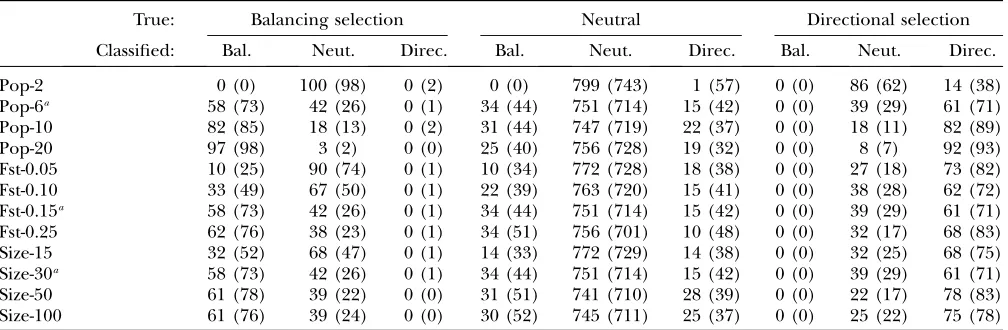
SNP simulation results
True: Balancing selection Neutral Directional selection
Classified: Bal. Neut. Direc. Bal. Neut. Direc. Bal. Neut. Direc.
Pop-2 0 (0) 100 (98) 0 (2) 0 (0) 799 (743) 1 (57) 0 (0) 86 (62) 14 (38) Pop-6a 58 (73) 42 (26) 0 (1) 34 (44) 751 (714) 15 (42) 0 (0) 39 (29) 61 (71) Pop-10 82 (85) 18 (13) 0 (2) 31 (44) 747 (719) 22 (37) 0 (0) 18 (11) 82 (89) Pop-20 97 (98) 3 (2) 0 (0) 25 (40) 756 (728) 19 (32) 0 (0) 8 (7) 92 (93) Fst-0.05 10 (25) 90 (74) 0 (1) 10 (34) 772 (728) 18 (38) 0 (0) 27 (18) 73 (82) Fst-0.10 33 (49) 67 (50) 0 (1) 22 (39) 763 (720) 15 (41) 0 (0) 38 (28) 62 (72) Fst-0.15a 58 (73) 42 (26) 0 (1) 34 (44) 751 (714) 15 (42) 0 (0) 39 (29) 61 (71) Fst-0.25 62 (76) 38 (23) 0 (1) 34 (51) 756 (701) 10 (48) 0 (0) 32 (17) 68 (83) Size-15 32 (52) 68 (47) 0 (1) 14 (33) 772 (729) 14 (38) 0 (0) 32 (25) 68 (75) Size-30a 58 (73) 42 (26) 0 (1) 34 (44) 751 (714) 15 (42) 0 (0) 39 (29) 61 (71) Size-50 61 (78) 39 (22) 0 (0) 31 (51) 741 (710) 28 (39) 0 (0) 22 (17) 78 (83) Size-100 61 (76) 39 (24) 0 (0) 30 (52) 745 (711) 25 (37) 0 (0) 25 (22) 75 (78)
Numbers of SNP loci simulated under (‘‘true’’) balancing selection, neutrality, and directional selection that were classified in each category using a reversible-jump cutoff of 0.86 (0.79) that give false-positive rates of 5% (10%) are shown. Bal., balancing selection; Neut., neutrality; Direc., directional selection.
a
rate. However, for balancing selection, we need 10 populations with AFLPs and SNPs to reach a compara-ble result. Microsatellites, on the other hand, perform fairly well even with only 2 populations.
The level of genetic differentiation also plays an important role for the detection of balancing selection. Weak genetic differentiation (FST # 0.05) makes it
almost impossible to detect balancing selection with AFLP or SNP data. On the other hand, with micro-satellites, even a small amount of genetic differentiation
FST¼0.01 allows us to detect balancing selection. Here
we did not note a negative influence of high genetic differentiation on the detection of directional selection but we conducted further simulations (not presented here) with only two populations, and, in that case, having a high genetic differentiation (0.25) leads to low power to detect directional selection.
The sample size is also important for the detection of balancing selection. The lower false-positive rate ob-served in cases of small sample size is due to the lack of
power of the method to detect any loci under selection (being true or false positives). For directional selection, increasing the sample size is less valuable; it is possible to obtain a correct true-positive rate with only 15 individ-uals per population for AFLPs or SNPs and with only 10 individuals per population for microsatellites. Note that this result is valid only because we used six populations and FST ¼0.15; but, for example, if we had only two
populations and a higher genetic differentiation, it would be necessary to have larger sample sizes.
In terms of the effect of inbreeding on the power to detect selection using dominant markers such as AFLPs, the results are very similar for all theFISvalues
considered (Table 3), which suggests that inbreeding is not an issue for the application of our method.
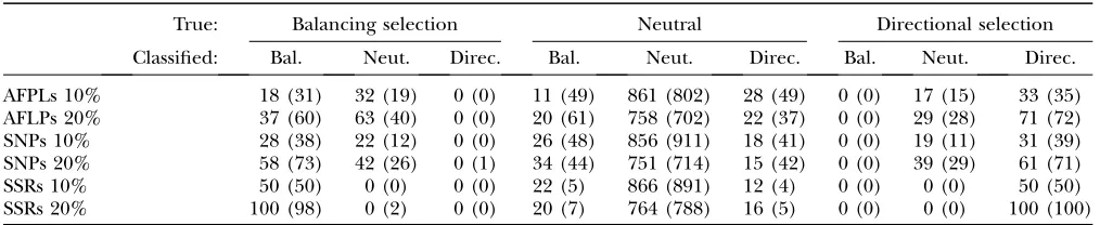
It is possible that the false-positive rate is influenced by the proportion of selected loci in the genome. Thus, we carried out additional simulations with a smaller proportion (10%) of loci under selection for the default scenario with six populations for AFLPs and SNPs
TABLE 5
Microsatellite simulation results
True: Balancing selection Neutral Directional selection
Classified: Bal. Neut. Direc. Bal. Neut. Direc. Bal. Neut. Direc.
Pop-2 75 (47) 25 (53) 0 (0) 23 (4) 765 (792) 12 (4) 0 (0) 3 (12) 97 (88) Pop-4 100 (98) 0 (2) 0 (0) 20 (7) 764 (788) 16 (5) 0 (0) 0 (0) 100 (100) Fst-0.01 27 (1) 73 (99) 0 (0) 21 (1) 763 (793) 16 (6) 0 (0) 0 (1) 100 (99) Fst-0.03 90 (67) 10 (33) 0 (0) 35 (12) 744 (782) 21 (6) 0 (0) 0 (0) 100 (100) Fst-0.05 100 (100) 0 (0) 0 (0) 17 (9) 761 (786) 22 (5) 0 (0) 0 (0) 100 (100) Size-10 97 (88) 3 (12) 0 (0) 17 (2) 761 (792) 22 (6) 0 (0) 0 (0) 100 (100) Size-15 100 (100) 0 (0) 0 (0) 20 (6) 766 (791) 14 (3) 0 (0) 0 (0) 100 (100) Alpha-0.5 31 (13) 69 (87) 0 (0) 25 (4) 755 (792) 20 (4) 1 (0) 49 (69) 50 (31) Alpha-1.0 92 (79) 8 (21) 0 (0) 15 (3) 762 (791) 23 (6) 0 (0) 7 (14) 93 (86) Alpha-1.5 100 (97) 0 (3) 0 (0) 22 (4) 761 (792) 17 (4) 0 (0) 0 (2) 100 (98)
Numbers of microsatellites loci simulated under (‘‘true’’) balancing selection, neutrality, and directional selection that were classified in each category using a reversible-jump cutoff of 0.85 (0.98) are shown. The 0.85 cutoff gives the same false-positive rate of 5% used for AFLP and SNP data sets. The 0.98 cutoff gives a false-positive rate of only 1%. Bal., balancing selection; Neut., neutrality; Direc., directional selection.
TABLE 6
Simulation results when 10% of the loci are subjected to selection
True: Balancing selection Neutral Directional selection
Classified: Bal. Neut. Direc. Bal. Neut. Direc. Bal. Neut. Direc.
AFPLs 10% 18 (31) 32 (19) 0 (0) 11 (49) 861 (802) 28 (49) 0 (0) 17 (15) 33 (35) AFLPs 20% 37 (60) 63 (40) 0 (0) 20 (61) 758 (702) 22 (37) 0 (0) 29 (28) 71 (72) SNPs 10% 28 (38) 22 (12) 0 (0) 26 (48) 856 (911) 18 (41) 0 (0) 19 (11) 31 (39) SNPs 20% 58 (73) 42 (26) 0 (1) 34 (44) 751 (714) 15 (42) 0 (0) 39 (29) 61 (71) SSRs 10% 50 (50) 0 (0) 0 (0) 22 (5) 866 (891) 12 (4) 0 (0) 0 (0) 50 (50) SSRs 20% 100 (98) 0 (2) 0 (0) 20 (7) 764 (788) 16 (5) 0 (0) 0 (0) 100 (100)
and four populations for microsatellites (see Table 2). The false-positive and false-negative rates are similar to those observed when 20% of the loci are under selection (see Table 6). This is another advantage of the model proposed by Beaumont and Balding (2004) that we
use here over previous approaches. As explained in the Introduction, this is due to the fact that this model does not require us to input parameters estimated on neutral markers that could be biased by the presence of a high number of selected loci (Beaumontand Nichols1996;
Vitaliset al.2001).
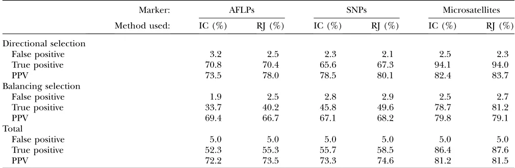
Comparison with Beaumont and Balding’s (2004)
method: Instead of using an approach to estimate the
probability thataiis different from 0, such as the one we propose here, Beaumontand Balding(2004) adopted
a simple informal criterion for identifying values ofai that are ‘‘significant.’’ More precisely, they defineaito be ‘‘significant at levelP’’ if its equal-tailed 100(1 –P)% posterior interval excludes zero. For example, ifP¼5%, then ai is significantly positive if its 2.5% quantile is positive and is significantly negative if its 97.5% quantile is negative. In the former case we would conclude that the locus is subjected to directional selection while in the latter we would conclude that it is subjected to balancing selection. We use the three series of data sets presented above to compare the two different ways of detecting selection. We applied the informal criterion on all these simulated data sets using the same false-positive rate of 5% (it corresponds, respectively, to a cutoff value of the informal criterion of 0.95, 0.96, and 0.98 for AFLPs, SNPs, and microsatellites). A summary of the results is presented in Table 7. The global PPVs are sightly higher for the reversible jump than for the informal criterion in seven of the nine cases. The results are very similar between the two approaches for
micro-satellites and the new method seems to be particularly useful for AFLPs and SNPs.
Spatial population expansion model: The results of the
simulations show that sampling design can affect the ability of our method to detect outliers. Indeed, even though we used a neutral mutation model to generate the synthetic data, we identified loci that had a posterior probability.0.99 of being outliers. More precisely, we observed 3.5, 3.0, 2.2, and 1.7% of false positives for scenarios based on the HGDP–CEPH data set with 53, 26, 22, and 19 populations, respectively. Addition-ally, the scenario with uniform sampling led to a false-positive rate of 10.6%.
Including markers with different mutation rates can also affect the performance of our method. The analysis that included all 3000 loci without distinguishing between di-, tri-, or tetranucleotides led to a false-positive rate of 2.2%. On the other hand, carrying out separate analyses for each type of microsatellite and then pooling the results led to a false-positive rate of 1.6%. Additionally, the simulations allowing for variable mutation rates within each class of microsatellite led to 4.5% false positives when carrying out a separate analysis for each type and to 5.6% when analyzing all 3000 markers simultaneously.
Our results are in accordance with those of Currat
et al.(2006), showing that severe population bottlenecks
during a geographic expansion can lead to false-positive detection of selection. However, this problem can be avoided by excluding isolated populations from the analysis. In the case of humans, this is done by consid-ering only the 19 continental populations of Africa, Europe, and Asia. It is worth emphasizing that a uniform sampling design that includes many isolated popula-tions is likely to lead to a high false-positive rate and,
TABLE 7
Simulation results summary
Marker: AFLPs SNPs Microsatellites
Method used: IC (%) RJ (%) IC (%) RJ (%) IC (%) RJ (%)
Directional selection
False positive 3.2 2.5 2.3 2.1 2.5 2.3
True positive 70.8 70.4 65.6 67.3 94.1 94.0
PPV 73.5 78.0 78.5 80.1 82.4 83.7
Balancing selection
False positive 1.9 2.5 2.8 2.9 2.5 2.7
True positive 33.7 40.2 45.8 49.6 78.7 81.2
PPV 69.4 66.7 67.1 68.2 79.8 79.1
Total
False positive 5.0 5.0 5.0 5.0 5.0 5.0
True positive 52.3 55.3 55.7 58.5 86.4 87.6
PPV 72.2 73.5 73.3 74.6 81.2 81.5
therefore, should be avoided. Finally, we showed that including in the same analysis loci with different mutation rates can also increase the false-positive rate. For microsatellites, performing separate analyses on di-, tri-, and tetranucleotides solves this problem, but biases due to variable mutation rate within each class of microsatellite are difficult to avoid.
APPLICATION
Humans:We use the HGDP–CEPH Human Genome Diversity Cell Line Panel presented by Cannet al.(2002)
to identify regions of the human genome that may be influenced by selection. The last version of this data set consists of 1056 individuals from 53 subpopulations, which were scored for 835 microsatellites. On the basis of the results of our realistic simulation study, we chose to use the same 19 continental populations from Africa, Europe, and Asia to minimize the false-positive rate. We kept only microsatellites that were strictly di-, tri-, and tetranucleotidic, which led us to select 106 dinucleo-tides, 127 trinucleodinucleo-tides, and 327 tetranucleodinucleo-tides, leading to a total of 560 markers. To further minimize the detection of false positives we adopted the best strategy identified by our simulations and conducted separated analyses for each of the three types of markers and grouped the results. We used the same cutoff value of 0.99 as in the simulated data set. We found 131 loci under selection: 86 were detected as being under directional selection and 45 under balancing selection.
This represents 23% of the studied loci and is much higher than the false-positive rate estimated from the simulation study that considered similar demographic and sampling scenarios (4.5%). These results suggest that a high number of loci have been subject not only to directional (15%) but also to balancing selection (8%) in the course of human evolution.
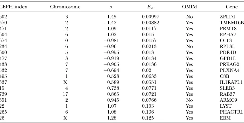
We identified the microsatellite loci that are located within a gene whose position is well defined, using the NCBI UniSTS database (http://www.ncbi.nlm.nih.gov/ sites/entrez?db¼unists). We found eight microsatellites close to known genes under directional selection of which two were located on the X chromosome and 10 known genes under balancing selection, all located on autosomes (Table 8). We then used the Online Mende-lian Inheritance in Man (OMIM) database (ftp.ncbi. nih.gov/repository/OMIM/morbidmap) to establish the putative function of the 18 genes identified using NCBI and established that 15 genes (8 under balancing and 7 under directional selection) are referenced as implicated in a genetic disease. These results are in accordance with those of Clark et al. (2003) who
showed that the genes under selection are overrepre-sented in this database.
Littorina saxatilis:To present an application to AFLPs,
we reanalyzed theLittorina saxatilisdata set of Wilding
et al.(2001), studied also by Grahameet al.(2006). The
data consist of 290 polymorphic AFLP loci, surveyed in four different rocky shores in Britain: Thornwick Bay, Flamborough (TH); Filey Brigg (FY); Old Peak (OP); and Robin Hood’s Bay (RB). In this regionL. saxatilisis
TABLE 8
Genes under natural selection
CEPH index Chromosome a FST OMIM Gene
602 3 1.45 0.00997 No ZPLD1
570 12 1.42 0.00882 Yes TMEM16B
471 12 1.09 0.0117 Yes PRMT8
604 6 1.02 0.015 Yes EPHA7
674 10 0.981 0.0157 Yes OIT3
234 16 0.96 0.0213 No RPL3L
600 5 0.955 0.013 Yes PDE4D
477 3 0.919 0.0134 Yes GPD1L
433 7 0.905 0.0136 Yes PRKAG2
532 7 0.694 0.02 Yes PLXNA4
495 1 0.523 0.0633 Yes C8B
337 X 0.589 0.0551 Yes IL1RAPL1
15 4 0.738 0.0771 Yes SLEB3
739 17 0.865 0.0721 Yes RAB37
351 2 0.945 0.0766 No ARMC9
22 1 1.07 0.103 Yes LYST
265 6 1.08 0.136 Yes PHACTR1
26 X 1.28 0.125 Yes EBM
Genes identified as under balancing (a,0) and directional (a.0) selection with the corresponding pos-terior estimate ofFSTare shown. Highest absolute values ofasuggest a stronger effect of selection. For each
found as two morphological forms (‘‘H’’ and ‘‘M’’) that show good evidence of partial reproductive isolation. One set of individuals of each morphological form was sampled in each shore, with the exception of the RB shore where two sets of M were sampled. Each of the eight resulting samples is composed of 43–51 individuals.
In each shore two hypotheses can explain the observed divergence between the two morphological forms (Grahameet al.2006): an allopatric divergence
followed by a secondary contact or a primary parapatric divergence (Wilding et al. 2001). In both cases
pop-ulations are likely to be exchanging genes only in the region of contact, and using the eight populations in a single analysis would lead to a violation of the de-mographic model assumed by our inference method. This is also supported by the neighbor-joining tree constructed by Wildinget al.(2001) from the loci they
identified as neutral: populations were clustered by site (they also constructed a tree using all loci, which led to a grouping of populations by morphotypes H and M).
Wildinget al.(2001) used a modified version of the
Fdist model (Beaumont and Nichols1996) to detect
selection from dominant markers. They analyzed three data sets, corresponding to the three shores where both morphotypes were sampled, each one containing two populations. One potential problem of the Beaumont
and Nichols(1996) method is the necessity to estimate Nmfrom the data set to perform simulations with this target value. However, the estimation of Nm assumes neutrality and is overestimated in the presence of di-rectional selection. To avoid this problem, they used an iterative procedure whereby the mean FSTcalculated
from the full data set is used as input of a first Fdist run, and then it is iteratively modified as outlier loci are removed. After four such steps, Wilding et al.(2001)
retained only loci that were lying above the 0.99 quantile in all three H–M comparisons and identified 15 loci under selection.
We made the same three analyses of each two-population data set using our method. The Bayesian model we used takes explicitly into account the loci under selection in the estimation ofFSTcoefficients in
Equation 3 and, therefore, does not suffer from the problem mentioned above. Beaumont and Balding
(2004) compared the criticalP-values between the Bayes-ian method and Fdist by matching the false-positive rate of 6800 neutral loci. They showed that a level of 1% for Fdist is equivalent to a level of 10% for the Bayesian model. Here, the sensitivity study above indicates that a 10% level for the informal criterion used by Beaumont
and Balding(2004) is equivalent to a cutoff value of 0.7
for the posterior probability estimated by our reversible-jump version of the method. We identified 13 loci with a probability.0.7 and they all belong to the list of 15 loci identified by Wildinget al.(2001). The two missing loci
are named ‘‘A37’’ and ‘‘F11’’ by Wildinget al.(2001)
and, according to our method, both are identified as outlier in only two of the data sets. More precisely, the A37 locus has a posterior probability of only 0.53 in the Filey data set, and the F11 locus has a posterior probability of 0.65 in the Old Peak data set. These loci are at the lower tail of the allele-frequency distribution estimated by Wildinget al.(2001) in two of the three
data sets considered. If we were to use a cutoff value of 0.65 instead of 0.7 we would include the F11 locus in the list of selected loci but also an additional marker not found by Wildinget al.(2001).
We also analyzed these three sets of two populations as a single data set of six populations to investigate the influence of the violation of the demographic model assumed by our method. Using a cutoff value of 0.99, all 13 loci found in the pairwise analyses are identified as outliers, but we also find 4 additional loci. The results of the simulations of the spatial expansion model suggest that these loci could be false positives due to the violation of the demographic model assumed. As was the case for the human data set, these 4 loci have a posterior estimate ofasituated at the tail of the distribution ofa-values for loci with a posterior probability .0.99. More precisely, the maximum estimated value ofafor these 4 additional loci is 1.89, while most of the loci identified as outliers (7 of 13) in the pairwise analyses have a posterior estimate ofagreater than this value.
To establish which of the two approaches is the most appropriate one, we modified the simulation scheme presented above to incorporate a different demo-graphic scenario. More precisely, instead of simulating the six populations under an island model, we simulated first three populations from this model (for the three shores) and then, from each one of them, generated allele frequencies for two populations (corresponding to the two different morphotypes). This demographic history mimics the neighbor-joining tree constructed by Wildinget al. (2001) from the loci they identified as
neutral. We chose simulation parameters to obtain data sets close to the real one. We simulated 290 such loci and 50 individuals in each population. We used FST¼0.05
between the ancestral population and the three in-termediate populations and FST ¼ 0.03 between the
intermediate populations and the six populations sam-pled. The ancestral allele frequencies were simulated from a beta distribution with both parameters equal to 0.5 and we choseFIS¼0.5. We added selection to 20 loci,
usinga¼2.5.
loci. The maximum estimated value of a for these 4 additional loci is 2.02, while only 11 of the 20 true outlier loci have a posterior estimate of a greater than this value. These results suggest that, under this particular demographic model, it is better to carry out pairwise analyses instead of a single global one. Moreover, it seems that the best strategy is to identify as selected all loci that are outliers in at least two of the three pairwise analyses. Indeed, if we use such an approach, then we retrieve all 20 loci under selection without identifying any false positives. Note that we can obtain the same result even if we raise the cutoff probability to 0.78.
Applying this approach to the periwinkle data set of Wildinget al.(2001), we identify as selected all 15 loci
originally found by them and also 6 additional outliers. We obtain the same result even if we raise the cutoff probability to 0.81. Thus, our analyses suggest that a total of 21 loci are influenced by selection in this species.
DISCUSSION
We present an extension of Beaumontand Balding’s
(2004) method to detect outlier loci that is applicable to both dominant and codominant markers. Additionally, we propose a rigorous way of estimating the posterior probability of a given locus being under the effect of selection. In their original formulation, Beaumont
and Balding(2004) focus on the posterior distribution
of locus-specific effects, ai, and use an approximate method to determine if a given locus is significantly in-fluenced by selection. On the other hand, the RJMCMC method we implemented is based on the idea that Equation 3 can give rise to two models, a null model
M0that includes only population-specific effects and an
alternative model M1 that includes both locus- and
population-specific effects. Thus, it is possible to directly estimate the posterior probability of each alternative model and on the basis of them decide which are the loci subject to selection. The main difference between the two methods is that the original one uses a cutoff value based on the false-positive rate that one is willing to accept. For example, if the threshold value is 99%, we expect to have 1% of false positives. However, one is not able to determine what is the probability that a given locus is or is not influenced by selection. In this sense, Beaumont and Balding’s (2004) approach uses the
same strategy as that of frequentist methods, where the objective is to reject a null hypothesis without being able to estimate what is the probability that this hypothesis is true. Our method, being fully Bayesian, allows us to rigorously estimate both P(ai ¼ 0 j data) [from the posterior probabilityP(M0jdata)] andP(ai6¼0jdata) [from the posterior probabilityP(M1j data)]. Once a
locus has been identified as being influenced by selection on the basis ofP(M1jdata) we can determine
if it is under balancing or directional selection using the mode of the posterior distributionP(ai jdata); a
neg-ative value indicates the former while a positive value indicates the latter.
Recently Riebleret al.(2008) presented an
approx-imate method to identify nonneutral loci that is not based on the posterior distribution ofai. They propose to introduce a Bernoulli-distributed auxiliary variable,di to indicate whether or not a locus is subjected to selection. Then, they classify a locus i as being under selection if the posterior probabilityP(di¼1jdata) is larger than a threshold value that is set by means of a simulation study. The authors propose to use a cutoff value of 0.17 based on simulations of a selective sweep under a Wright–Fisher model. The problem with this approach is that it is unlikely that this cutoff value is generally applicable to all data sets and all demographic scenarios. Additionally, it is clear thatP(di¼1jdata) cannot be interpreted as the probability that the locus is under selection; the most we can say is that it is proportional to this probability. Otherwise, it would imply that we are willing to accept that a locus is non-neutral even if the probability for this to be true is as low as 0.17. Our method, on the other hand, directly estimates this probability and allows us to avoid the use of simulations to choose a cutoff value. Of course, our method would still need simulations to adjust this cutoff value in cases of strong violation of the de-mographic model assumed, like we did for the human case.
With our approach, it is clear that for good-quality data we should choose a stringent criterion such as
P(ai 6¼0j data) $ 0.99, which leaves very little room for false positives. Of course, as our simulation study suggests, we may want to choose a somewhat lower threshold (e.g., 0.95) for dominant markers to take into account the fact that they are less informative than codominant ones. The full Bayesian estimation of the probability that a locus is influenced by selection pro-vided by our method also allows the consideration of other factors when choosing a cutoff value. For exam-ple, if the purpose is to study local adaptation using a model species for which many genetic resources exist, we may be willing to use a not very stringent criterion (e.g., 0.90) because the costs associated with localizing the position of the candidate loci for subsequent sequencing may not be too high. On the other hand, if we are dealing with a nonmodel species, we may want to use a very restrictive criterion [e.g.,P(ai6¼0jdata)$ 0.99 or 0.999] for deciding whether or not the species in question is appropriate for a study of local adaptation, based on the number of candidate loci found in a genome scan.