ABSTRACT
PONGPANICH, MONNAT. On the SNP-based and Sequence-based Whole Genome Studies for Complex Traits. (Under the direction of Dr. Jung-Ying Tzeng.)
Quality Control (QC) of the single nucleotide polymorphism (SNPs) used in
genome-wide association studies (GWAS) is essential to minimize potential false findings. SNP QC commonly uses expert-guided filters to exclude low-quality SNPs. Expert filters
aim to remove SNPs that fall into the extremes of QC variables including Hardy–Weinberg equilibrium, missing proportion (MSP) and minor allele frequency (MAF). However, implementations of these filters require arbitrary thresholds and do not jointly consider all
QC features. We propose an algorithm that is based on principal component analysis and clustering analysis to detect low-quality SNPs. The method minimizes the use of arbitrary
cutoff values, allows a collective consideration of the QC features and provides conditional thresholds contingent on other QC variables. We compare the performance of our method to expert filters on datasets from the Wellcome Trust Case Control Consortium and the Genetic
Association Information Network. Our results suggest that with the same or fewer SNPs excluded, the proposed algorithm tends to give a similar or lower inflation factor of the test
statistics (λ), gives a reduced number of false associations, and retains all true associations. GWAS methods that collapse information across genetic markers when searching for association signals are gaining momentum in the literature due to their usefulness in marker
set analysis and identifying rare variants. Collapsing information can be done at the genotype level, which focuses on the mean of genetic information or the similarity level, which focuses
underlying genetic architecture of the causal variants are the two factors that dominate their performance. Genotype collapsing is more sensitive to the marker set being contaminated by
noise loci than similarity collapsing. It performs best when the genetic architecture of the causal variants is not complex. Similarity collapsing is more robust and outperforms genotype collapsing when the genetic architecture of the markerset becomes more
sophisticated such as causal loci with various effect sizes or frequencies. In addition, we consider a two-stage analysis that combines the two top-performing methods from different
collapsing strategies and find that it is reasonably robust across all simulated scenarios. RNA-Seq is a promising approach for understanding transcriptomes due to its
accuracy, large dynamic range of expression level, and ability to detect novel transcripts. The
first step prior to any data analysis is to map reads against a reference genome or transcript set using an alignment tool e.g., TopHat. In many experiments, a non-trivial number of reads
are unmapped and excluded from down-stream analyses. To maximize the potential utility of sequenced reads, we propose a method of incorporating these unmapped reads in testing for differentially expressed (DE) genes. Specifically, we use BLAST to align the unmapped
reads and assign a weight to each mapped read that reflects the mapping confidence. Gene expression is estimated from the summation of weights of the reads mapped to a gene. To
test the general utility of the proposed approach, we construct a simple statistical method and show that using weights improves the power to detect DE genes while still controlling the false discovery rate. In addition, we examine the characteristics of the reads not mapped by
© Copyright 2012 by Monnat Pongpanich
On the SNP-based and Sequence-based Whole Genome Studies for Complex Traits
by
Monnat Pongpanich
A dissertation submitted to the Graduate Faculty of North Carolina State University
in partial fulfillment of the requirements for the degree of
Doctor of Philosophy
Bioinformatics
Raleigh, North Carolina 2012
APPROVED BY:
_______________________________ ______________________________
Dr. Jung-Ying Tzeng Dr. Dahlia Nielsen
Chair of Advisory Committee
DEDICATION
To my parents, for their unconditional love, encouragement and support.
BIOGRAPHY
Monnat Pongpanich was born in Bangkok, Thailand. She received her Bachelor of
Science in Computer Science from Chulalongkorn University in March 2005. Shortly after she joined ExxonMobil Limited in April 2005, she received a prestigious scholarship from Anandamahidol Foundation under the Royal Patronage of His Majesty the King of Thailand
to pursue a Ph.D. in Bioinformatics. She began her graduate work in Bioinformatics program at North Carolina State University in the summer of 2006. After receiving her doctoral
ACKNOWLEDGMENTS
I would like to express my gratitude to my advisor, Dr. Jung-Ying Tzeng, for her
guidance, patience and generous support. I am so thankful having her as my advisor. I can never thank her enough for all she has done for me. I would like to thank Dr. Dahlia Nielsen for her support and giving me the opportunity to work on RNA-Sequencing project. She has
always been helpful and understanding. I would also like to thank Dr. Steffen Heber for his time, advice and contribution on my first project. I would also like to thank Dr. Trudy
Mackay for her comments and taking the time to serve in my committee. My sincere appreciation is extended to Dr. Patrick Sullivan. I have learned many things from his lab. I would also like to thank Dr. John Pierre Mertz for correcting grammar in my first research
paper.
I am also extremely grateful for the financial support from Anandamahidol
Foundation. My graduate study would not have begun without Anandamahidol Foundation. I would like to thank Dr. Nalin Nilubol for being my caring mentor. Thank you to Ms.
Komsorn Aukayapisudhi for all the administrative help. I also gratefully acknowledge
financial support from the National Institutes of Health (grant R01 MH084022-01A1). Thank you to Sirote Chaiwattanapong for being by my side and making me happy.
Thank you to Santi Sanglestsawai for taking good care of me and helping me in ST521 and ST522. Thank you to Plawut Wongwiwat for making me feel that everything will be okay when I am panic. Thank you to Adisri Charoenpanich for being my girlfriend. Thank you to
Warakorn Bunkanokwong, Sitthichai Tanthasith, Sirapun Yongwattananunth, Piyada
Sasitorn Srisawadi, Manida Swangnetr and Karnjana Sanglimsuwan for settling me down here. Thank you to Ganokon Urkasemsin for always listening to me. Thank you to Worawut
Wangwatcharakul and Raywat Tanadkithirun for helping me with statistics.
I also appreciate the support from the faculty and staffs at the Bioinformatics Research Center. Thank you to Chris Smith for all your help from technical support to
correcting my English grammar. Thanks to Julibeth Briseno and Siarra Dickey for all the administrative help and Tina Chen for handling all my financial documents.
A special thanks to Noffisat Oyindamola Oki, Gunjan Hariani, Nicholas Hardison, Alexander Griffing, Xin Wang, Zhi Wang, Youfang Liu, Megan Neely, Jihye Kim, Ronglin Che, Chen-yen Lin and Na Cai for all their help and wonderful friendship.
Lastly and most importantly, I would like to thank my parents, Tanong and Gridsana Pongpanich, and Panitan Patrayunyong. You are there for me 24/7. You give me strength,
TABLE OF CONTENTS
LIST OF TABLES ... ix
LIST OF FIGURES ... x
Chapter 1: Introduction ... 1
Association Studies ... 1
Obtaining genotypes. ... 2
SNP array. ... 2
DNA sequencing. ... 4
Quality control. ... 6
Detecting association. ... 7
Gene Expression ... 8
Overview of the Dissertation ... 11
References ... 13
Chapter 2: A Quality Control Algorithm for Filtering SNPs in Genome-wide Association Studies ... 19
Abstract ... 19
Introduction ... 20
Methods... 23
The proposed QC algorithm... 23
Performance evaluations using real datasets. ... 26
Implementation. ... 27
Results ... 28
Discussion ... 30
Table ... 34
Supplementary tables ... 35
Figures... 43
Supplementary Figures ... 47
References ... 61
Chapter 3: On the Aggregation of Multimarker Information for Marker-set and Sequencing Data Analysis: Genotype Collapsing vs. Similarity Collapsing ... 64
Abstract ... 64
Materials and Methods ... 68
Methods... 69
Single SNP-based marker-set test: MinP. ... 69
Combined multivariate and collapsing method. ... 70
Variable threshold method. ... 70
Gene-trait similarity regression... 71
Simulation studies. ... 72
Simulation settings. ... 72
Data generation. ... 74
Computational details. ... 75
Results ... 76
Underlying genetic architecture. ... 77
Causal allele frequency (Figures 1 and 6)... 77
Magnitude of causal allele effect (Figures 2 vs. 1 and 7 vs. 6)... 78
Multiple causal alleles in a locus (Figures 3 vs. 1). ... 79
Composition of marker set. ... 79
Proportion of causal Loci (Figures 1, 4, 5, and 6). ... 79
LD between causal and non-causal loci (Figure 1). ... 80
Weighting schemes used in collapsing methods. ... 81
SimReg method. ... 81
SimReg0, SimReg3 vs. SimReg4. ... 81
Rare variants vs. all variants. ... 82
CMC method. ... 82
VT method. ... 83
Discussion ... 83
Tables ... 88
Figures... 89
References ... 96
Chapter 4: Assessing RNA-seq Differential Expression Levels with Low-confidence Mapped Reads ... 100
Introduction ... 100
Imposing quality weights to TopHap unmapped reads... 102
Characteristics of unmapped reads. ... 104
Statistical tests to detect DE genes... 105
Obtaining the null distribution of the test statistics. ... 107
Simulation design... 108
Results ... 110
Characteristics of unmapped reads by TopHat. ... 110
Simulation results... 112
False discovery rate... 113
Power to detect DE genes. ... 113
Discussion ... 115
Tables ... 118
Figures... 121
References ... 130
Chapter 5: Concluding Remarks ... 132
References ... 136
Appendix A: The Change-Point Model for Estimating r ... 138
Appendix B ... 140
B.1 The derivation of variance... 140
LIST OF TABLES
Chapter 2: A Quality Control Algorithm for Filtering SNPs in Genome-wide Association Studies
Table 1. Agreement and disagreement in SNP classifications (good SNPs versus bad SNPs) by the proposed filter and the WTCCC expert filter ... 34 Supplementary Table 1. Proportion of SNPs excluded and λ value of the proposed
filter and the WTCCC expert filters... 35 Supplementary Table 2. Counts of false positives (FP), true positives (TP) of the
proposed filter and the WTCCC expert filters ... 37 Supplementary Table 3. Agreement and disagreement in SNP classifications (good
SNPs vs. bad SNPs) by the proposed filter and the WTCCC expert filter ... 39 Supplementary Table 4. Agreement and disagreement in SNP classifications (good
SNPs vs. bad SNPs) by the proposed filter and the WTCCC expert-no-MAF filter (i.e., the expert filter without removing SNPs with MAF < 0.01). ... 41
Chapter 3: On the Aggregation of Multimarker Information for Marker-set and Sequencing Data Analysis: Genotype Collapsing vs. Similarity Collapsing
Table 1. Minor allele frequency (MAF) of markers resulting from sequencing data from the CHB sample of 1000 Genomes Project. ... 88 Table 2. Type I error rates averaged over the 495 possible scenarios for 4 causal
markers out of 12 and 500 replicate data sets. ... 88
Chapter 4: Assessing RNA-seq Differential Expression Levels with Low-confidence Mapped Reads
Table 1. Percentage of reads mapped by TopHat and BLAST ... 118 Table 2. Characteristics of reads unmapped by TopHat but mapped by BLAST
categorized into 16 types. ... 118 Table 3. Proportion of reads from each characteristic in human, M. truncatula, mouse and corn ... 119 Table 4. Estimated FDRs based on an average across 100 simulated datasets at five
nominal levels ... 119 Table 5. Power based on an average TPR across 100 simulated datasets at five
LIST OF FIGURES
Chapter 2: A Quality Control Algorithm for Filtering SNPs in Genome-wide Association Studies
Figure 1. Projections of SNPs on the two-dimensional PC plane for the WTCCC CAD study.. ... 43 Figure 2. Projections of SNPs on the two-dimensional PC plane for the GAIN MDD
study.. ... 44 Figure 3. Performance comparisons of different filters based on the four criteria
defined in the text... 45 Figure 4. Characteristics of SNPs with disagreeing classification results between the
proposed filter and WTCCC expert filter in CAD. ... 46 Supplementary Figure 1. Projections of SNPs on the 2-dimentional PC plane for BD,
CD, HT, RA, T1D, T2D and MDD.. ... 48 Supplementary Figure 2. Characteristics of SNPs with disagreed classification results
between the proposed filter and WTCCC expert filter for BD, CD, HT, RA, T1D and T2D. .. ... 54
Chapter 3: On the Aggregation of Multimarker Information for Marker-set and Sequencing Data Analysis: Genotype Collapsing vs. Similarity Collapsing
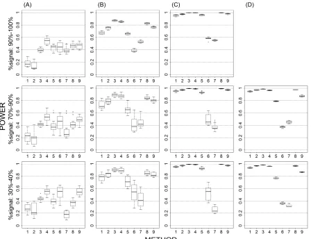
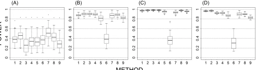
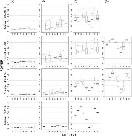
Figure 1. Power results when casual loci have same effects under 4 causal loci out of 12 markers setting for binary trait. ... 89 Figure 2. Power results when casual loci have different risk effect sizes under 4
causal loci out of 12 markers setting for binary trait. ... 90 Figure 3. Power results for multiple causal alleles in a locus with same effects under 4
loci out of 12 markers setting for binary trait. ... 91 Figure 4. Power results when casual loci have same effects under 4 causal loci out of
4 markers setting for binary trait. ... 92 Figure 5. Power results when casual loci have same effects under 2 loci out of 12
markers setting for binary trait. ... 92 Figure 6. Power results when casual loci have same effects under 2 loci out of 30
markers setting for binary trait. ... 93 Figure 7. Power results when casual loci have different risk effect sizes under 2 loci
out of 30 markers setting for binary trait. ... 94 Figure 8. Power results when casual loci have same effects under 2 loci out of 12
Chapter 4: Assessing RNA-seq Differential Expression Levels with Low-confidence Mapped Reads
Figure 1. An illustration of how differentially expressed genes are created. ... 121
Figure 2. Characteristics of reads mapped by BLAST in human ... 122
Figure 3. Characteristics of reads mapped by BLAST in M. truncatula ... 123
Figure 4. Characteristics of reads mapped by BLAST in mouse ... 124
Figure 5. Characteristics of reads mapped by BLAST in corn ... 125
Figure 6. Testing for differential expression using weighted counts. ... 126
Figure 7. Testing for differential expression using unweighted counts. ... 127
Figure 8. log2 of foldchange between weighted and unweighted counts. ... 128
Figure 9. log2 of mean normalized expression between weighted and unweighted counts. ... 129
Chapter 1
Introduction
Association Studies
A genetic association study aims to find associations between genetic
polymorphism(s) and phenotypes (Lunetta, 2008). In family-based association studies, the transmission frequency for each allele from heterozygous parent to affected offspring is
estimated and is 50% under the null. In contrast, disease associated alleles will be transmitted in excess to the affected individual. The challenge in this design is its sensitivity to
genotyping error which can distort transmission proportions between parents and offspring (Pearson & Manolio, 2008). In case-control association studies, the allele or genotypes frequencies between cases and controls are compared (Hirschhorn & Daly, 2005). If the
variant does not relate to the disease, the alleles/genotypes frequencies between cases and controls should not significantly differ. This design is susceptible to population substructure
(McCarthy et al., 2008) and additional procedures must be used to avoid spurious
association, such as computing association statistics that take subpopulation clusters into account (Pritchard et al., 2000), adjusting for the inflation factor caused by the substructure
(Devlin & Roeder, 1999), and using major principal components as covariates to correct for stratification (Price et al., 2006). Prior to next generation sequencing technologies,
(Neale & Purcell, 2008) and association studies have identified many common alleles
associated with disease (Donnelly, 2008; Hardy & Singleton, 2009). Nevertheless, proportion
of heritability explained by the loci found in association studies is small. For example, in a GWAS study of a highly heritable trait, height, 180 loci have been identified, yet proportion of heritability explained is only 10% (Allen et al., 2010). Much of the speculation is that rare
variants contribute to the missing heritability (Bogardus, 2009; Manolio et al., 2009). The individually trivial contributions of rare variants to the proportion of the variance in a trait,
and their low frequency, make it difficult to detect rare variants by association studies based on the use of tag SNPs (Bodmer & Bonilla, 2008). Direct sequencing of candidate gene or the entire genome allows us to identify rare variants. In the near future, sequencing
technologies will become more cost-effective. This starts to shift the first wave of association studies to re-sequencing association studies or DNA sequence-based association studies. The
voluminosity and new type of data (sequence reads) having a wide spectrum of allele frequencies coming from sequencing poses many challenges: (a) storing, accessing, and handling data; (b) mapping short reads to a reference genome or de novo assembly of the
genome; (c) calling true variants; (d) analyzing common and low frequency loci that may exhibit allelic heterogeneity with respect to the trait (Pop & Salzberg, 2008; Day-Williams &
Zeggini, 2011).
Obtaining genotypes.
SNP array. In high throughput SNP arrays, millions of SNPs are genotyped in a
of fragments, adaptors are then ligated to fragments regardless of size, fragments with selected size are amplified by PCR, and the amplified target is fragmented, denatured, end
labeled and hybridized to the array. The array contains the probes for each of the two SNP alleles (A, B) (Affymetrix, Inc., 2009).
For each SNP and each individual, probe hybridization intensities are summarized for
each allele. That is, a pair of coordinates - an “A” signal and a “B” signal, which correspond to the quantities of the “A” and “B” alleles, are obtained (Affymetrix Inc., 2007). Automated
procedures have been developed to call genotypes. Typically, they employ information across samples at each SNP. This usually results in three clouds of fluorescent signals where the cluster of points with high “A” (”B”) signal but close to zero “B” (”A”) signal is expected
to correspond to AA (BB) genotype samples and the cluster of points with similar “A” and “B” signal is expected to correspond to AB genotype samples (Teo, 2008). The genotype
clusters are used to call genotypes for each sample. Generally, the genotype calling algorithms calculate probabilities of belonging to each of the three clusters given the
observed data point across all samples and assign the most likely genotype to a sample if the
corresponding probability passes the threshold (e.g., WTCCC, 2007; Affymetrix Inc., 2007). Under ideal conditions, obtaining genotypes should be straightforward. However,
various factors can affect genotyping accuracy. For some SNPs, the three clusters overlap and thus cause ambiguity in calling the genotype, resulting in assigning “missing call” to individuals in the overlap regions (Anney et al., 2008). In some SNPs,
(Pompanon et al., 2005). The confidence score threshold is another factor that provides a tradeoff between call rate and accuracy (Teo, 2008). In addition, monomorphic SNPs can be
erroneously assessed as polymorphic (Pettersson et al., 2008). The calling accuracy can also depend on batch composition (combining or separating cases and controls) and batch size (the number of samples called at the same time) especially for SNPs with low minor allele
frequency (MAF) as calling more people at the same time will help in forming the minor allele homozygote cluster (Teo, 2008; Miclaus et al., 2010).
DNA sequencing. Sequencing technologies differ in the specific protocols they
combine. Major steps are template preparation, sequencing and imaging, and genome alignment and assembly. There are two types of templates: clonally amplified and
single-molecule. In clonally amplified templates, the two most common methods, emulsion PCR (one DNA molecule per bead; beads are deposited into wells) and solid-phase amplification
(resulting in hundreds of millions of molecular clusters; one DNA molecule per cluster), can be used to amplify the DNA molecule. Amplification is necessary because the imaging systems cannot detect single fluorescent events (Metzker, 2010). In single-molecule
templates, the template molecules are immobilized on a solid support either via primer immobilization, template immobilization (Helicos BioSciences Corporation, 2008, 2010) or
polymerase immobilization (Pacific Biosciences, 2009).
Sequencing strategies can be divided into 4 types: cyclic reversible termination (CRT), sequencing by ligation (SBL), single nucleotide addition (SNA; pyrosequencing) and
a series of color images from each cluster are translated into a sequence as one color represents one base (Illumina, Inc., 2010). In one-color CRT, a series of light on and off
images from each cluster are translated into a sequence as nucleotides are flowed
sequentially in a specific order (Helicos BioSciences Corporatio, 2010). In SBL, two-base-encoded probes are used to interrogate two bases at a time. Five primer rounds are performed
(shifting primer one position to the left between each round).Color calls from five ligation rounds are compiled and decoded into DNA sequence (Life Technologies Corporation,
2011). In SNA, the emitted light is recorded as a series of peaks called a flowgram, which reveal the DNA sequence (Roche Diagnostics Gmb, 2006). In real time sequencing,
incorporation of nucleotides is continuous and sequential bursts of light are recorded (Pacific
Biosciences, 2009).
The output from sequencing is (potentially) millions of reads and associated quality
scores. The next step is to map these short reads to the reference genome or de novo assembly. The alignment step is important, as wrongly mapped reads will propagate error into downstream analysis (Day-Williams & Zeggini, 2011). There are numerous challenges
in the alignment step: reads may have sequencing errors, reads might map to multiple locations in the genome, reads may be from repetitive regions or might correspond to a
region that does not exist in the reference genome (Marguerat&Bähler, 2010; Metzker, 2010; Day-Williams &Zeggini, 2011). Once reads are mapped, the variants are called. However, complications in variant calling include alignment artifacts, PCR artifacts, and location of the
PCR reaction introduces reads supporting both the correct and erroneous bases, confident but spurious SNP calls could be generated. The ends of the reads can lead to false SNP calls as
error rates are higher for the bases toward the end of the reads (Day-Williams & Zeggini, 2011).
Quality control. In order that association studies have reliable and reproducible results, good quality control is essential. Genotyping error can alter the magnitude of the difference between allele frequencies incases and controls, thus affecting the power (Gordon
&Ott, 2001). Differential genotyping error rates between cases and controls can result in type I error (Moskvina et al., 2006; Clayton et al., 2005; Morris & Cardon, 2007).
Quality control is usually done in two levels: sample quality control and SNP quality
control. For sample quality control, samples with high rates of missingness or heterozygosity are excluded since high a missing proportion implies hybridization problems, and excess
heterozygosity is a sign of sample contamination. Related samples inferred through identity-by-state (IBS) are removed. Duplicate samples and samples with external discordance with genotype or phenotype data are also removed (Teo 2008; WTCCC, 2007). For SNP quality
control, expert filters are applied to SNPs in order to remove SNPs that fall into the extremes of QC variables including Hardy-Weinberg equilibrium (HWE), missing proportion (MSP),
and minor allele frequency (MAF). The rationale is clear: extreme deviation from HWE is typically used to identify gross genotyping error (Teo et al., 2007); a high MSP indicates poor genotype probe performance and low genotyping accuracy (Neale and Purcell, 2008;
with rare alleles (Neale and Purcell, 2008; Teo, 2008). After removing low quality SNPs, the presence of population structure in the data needs to be assessed and accounted for if present
in case-control studies. Once quality control is performed, researchers can then move on to association evaluation.
Detecting association. Methods for detecting marker association can be single-marker or multi-single-marker. In single-single-marker analysis, individual single-markers are tested for association. In multi-marker analysis, markers are grouped together into a marker-set and
association tests are performed for each marker-set. Marker sets can be formed based on functional annotations of the genomic regions e.g., grouping variants in regulatory regions or conserved regions, or grouping markers in the same gene or pathway, functionality of
variants e.g., grouping the coding variants, non-synonymous variants, or simply based on moving window or haplotype block (Bansal et al., 2010).
Although single-marker analysis has been successful in identifying many associated variants, marker-set analysis has an advantage over single-marker analysis (Wu et al., 2010). In single-marker analysis, the genome-wide significance threshold can be difficult to reach
due to the large number of tests. Marker-set analysis alleviates multiple testing problems (Wu et al., 2010, Tzeng et al., 2011). Marker-set analysis also enhances power to detect variants
as it accumulates small effects across multiple loci for common SNPs and enriches the signal in the case of rare variants, which are hard to detect via single-marker analysis. Marker-set analysis can also consider the joint effect of multiple markers that are potentially interacting
true effect more effectively as it is plausible that causal SNPs are in LD with many of markers in the set (Wu et al., 2010).
In a marker-set analysis, marker information in the set is aggregated and assessed for the collective effect of the markers on the phenotype. The information among markers can be collapsed at the genotype level or similarity level. Genotype collapsing methods focus on the
mean level of the genetic information, while similarity-collapsing methods focus on the variance level of the genetic information. At the genotype level, information can be collapsed
by calculating a weighted sum of the genotypes across all markers e.g., Li & Leal (2008), Madsen & Browning (2009), Han & Pan (2010), Price et al. (2010). At the similarity level, information can be collapsed by quantifying the genetic similarity across all markers for each
pair of unrelated individuals e.g., Wessel & Schork (2006), Tzeng et al. (2009, 2011),
Mukhopadhyay et al. (2010), Wu et al. (2010, 2011).The two collapsing paradigms have their
advantages and disadvantages. Researchers have to use their judgment to pick an appropriate method for their analysis.
Gene Expression
Genotypes give rise to phenotypes through gene expression. Previously, microarray allowed researchers to study gene expression for thousands of genes at once. However, the
introduction of massively parallel sequencing platforms has revolutionized the field. RNA-Seq is one of the applications of next generation sequencing. Microarrays are a hybridization-based approach and thus, suffer from background and cross-hybridization issues (Costa et al.,
2010). In contrast, RNA-Seq, based on the principles of DNA sequencing, has many
therefore detect novel transcribed regions. It does not have an upper limit for quantification, thus allows a large dynamic range of expression level (Wang et al., 2009). RNA-Seq results
show high levels of reproducibility (Marioni et al., 2008). Resolution of RNA-Seq data is a single base pair, consequently allowing researchers to generate annotation at single-base resolution e.g., transcript boundary (Wang et al., 2009; Costa et al., 2010). In addition, it
allows detection of antisense transcripts, SNPs and mutations (Wilhelm & Landry, 2009). In microarrays, RNA is extracted and labeled with a fluorescent dye. In two channel
microarrays, the treatment and control mRNA are labeled with two different dyes, mixed then hybridized on the same array. The array is scanned to acquire two images: treatment and control sample. In single channel microarrays, treatment and control are labeled with the
same dye but hybridized on different arrays (Tarca et al., 2006). The image is analyzed to obtain raw intensity data for every spot. The extracted data from the image is preprocessed to
filter poor quality data and then normalized. Finally, downstream analysis can be performed (Leung & Cavalieri, 2003).
In RNA-Seq, RNAs are isolated from cells and ribosomal RNAs (rRNA) are
removed. A library of cDNA fragments is prepared through either RNA fragmentation or DNA fragmentation. Sequencing adaptors are added to each cDNA fragment. The remaining
steps are as described in DNA sequencing: clonal amplification of cDNA fragments, sequencing and imaging the amplified fragments. The final output is millions of short sequence reads (Costa et al., 2010). The first step of any data analysis is either to map
post-transcriptionally modified e.g. alternative splicing (read spans exon junction),
polyadenylation and RNA editing, add more challenges (Marguerat & Bähler, 2010). At the
end of the alignment step, reads are either uniquely mapped, mapped to multiple locations (multi-match reads) or are not mapped (Costa et al., 2010). Most studies limit their attention to only uniquely mapped reads e.g., Nagalakshmi et al. (2008), Marioni et al. (2008).
However, there have been some efforts to address multi-match reads e.g., Cloonan et al.(2008), Faulkner et al.(2008), Mortazavi et al. (2008), Li et al. (2010).
To detect differentially expressed (DE) genes, gene expression must be quantified. Read counts are used to estimate gene expression and need to be properly normalized for two reasons: (1) longer transcripts generate more reads (2) number of fragment across samples
fluctuate for each run. Therefore, read counts are usually normalized by the gene’s length and total number of mapped reads in the sample. The expression of a gene is defined as the sum
of the expression level from all of its isoforms. Two schemes are most commonly used to obtain gene expression: (a) exon intersection method, which uses only constitutive exons and (b) exon union method, which uses exons from all isoforms (Garber et al., 2011). Regardless
of whether the exon intersection or union method is used, two approaches can be used to obtain the expression scores. One approach is to count the number of reads that cover each
nucleotide position within the included exons and then sum those counts. The other approach is to sum the number of reads that fall within the included exons. Then the sum is divided by the length of the feature and total number of reads mapped (Wilhelm & Landry, 2009).
microarrays, the output is fluorescent intensity, which can be effectively modeled as a continuous variable, whereas the count-based nature of RNA-Seq data needs to be modeled
as a discrete variable. Therefore, new methodologies have been developed to handle RNA-Seq data (Costa et al., 2010).In early attempts, the Poisson distribution was considered (Marioni et al., 2008), but it was found that the variation observed in RNA-Seq data are
larger than that predicted by Poisson (which is referred to as the overdispersion problem). More recent progress has focused on tackling this overdispersion problem based on modeling
counts using the negative binomial or the beta binomial, such as Robinson et al., (2010), Anders and Huber, (2010), Hardcastle and Kelly, (2010), Di et al., (2011) and Zhou et al., (2011).
Overview of the Dissertation
Genotype data quality is of paramount importance for association studies, thus
performing quality control is a preliminary step before testing for an association. The
arbitrary threshold and non-simultaneous consideration of all QC features has motivated us to develop an unsupervised filter based on the rationale of expert filters. In chapter 2, we
propose an algorithm that is based on principal component analysis and clustering analysis to identify low-quality SNPs. The method minimizes the use of arbitrary cutoff values, allows a
collective consideration of the QC features, and provides conditional thresholds contingent on other QC variables (e.g., different missing proportion thresholds for different minor allele frequencies).
weakness of the two collapsing paradigms: genotype collapsing vs. similarity collapsing, helps researchers select a suitable approach for their analysis. In chapter 3, we seek to
understand the advantages and drawbacks of the two collapsing paradigms over a wide range of plausible scenarios. We investigate the implications of employing these different
collapsing strategies when performing multi-marker association analysis.
In RNA-Seq analysis, read mapping is the first step prior to any analysis. Depending on the transcriptome and read length, the fraction of unmappable reads varies. Based on
analyses of a dataset from the Nielsen Lab, and many other experiments, this fraction is not trivial. Discarding these unmapped reads is wasteful in terms of cost and data loss. This has motivated us to minimize the amount of discarded data. In chapter 4, we incorporated reads
that an aligner tailored to short reads fails to map to detect DE genes by using a more general alignment algorithm i.e., BLAST, to align these unmapped reads and assign a weight to each
References
Affymetrix, I. (2007). BRLMM-P: A genotype calling method for the SNP 5.0 array. Retrieved 02/09, 2012, from
http://media.affymetrix.com/support/technical/whitepapers/brlmmp_whitepaper.pdf
Affymetrix, I. (2009). Data sheet: Genome-wide human SNP array 6.0. Retrieved 02/09, 2012, from
http://media.affymetrix.com/support/technical/datasheets/genomewide_snp6_datasheet.p df
Anders, S., & Huber, W. (2010). Differential expression analysis for sequence count data.
Genome Biology, 11, R106.
Anney, R. J. L., Kenny, E., O'Dushlaine, C. T., Lasky-Su, J., Franke, B., Morris, D. W., . . . Gill, M. (2008). Non-random error in genotype calling procedures: Implications for family-based and case-control genome-wide association studies. American Journal of Medical Genetics Part B: Neuropsychiatric Genetics, 147B, 1379-1386.
Bansal, V., Libiger, O., Torkamani, A., &Schork, N. J. (2011). An application and empirical comparison of statistical analysis methods for associating rare variants to a complex phenotype. Pacific Symposium on Biocomputing, 76-87.
Bodmer, W., & Bonilla, C. (2008). Common and rare variants in multifactorial susceptibility to common diseases. Nature Genetics, 40, 695-701.
Bogardus, C. (2009). Missing heritability and GWAS utility. Obesity, 17, 209-210.
Clayton, D. G., Walker, N. M., Smyth, D. J., Pask, R., Cooper, J. D., Maier, L. M., . . . Todd, J. A. (2005). Population structure, differential bias and genomic control in a large-scale, case-control association study. Nature Genetics, 37, 1243-1246.
Cloonan, N., Forrest, A. R. R., Kolle, G., Gardiner, B. B. A., Faulkner, G. J., Brown, M. K., . . . Grimmond, S. M. (2008). Stem cell transcriptome profiling via massive-scale mRNA sequencing. Nature Methods, 5, 613-619.
Costa, V., Angelini, C., De Feis, I., & Ciccodicola, A. (2010). Uncovering the complexity of transcriptomes with RNA-seq. Journal of Biomedicine and Biotechnology, 2010.
Devlin, B., & Roeder, K. (1999). Genomic control for association studies. Biometrics, 55, 997-1004.
Di, Y., Schafer, D. W., Cumbie, J. S., & Chang, J. H. (2011). The NBP negative binomial model for assessing differential gene expression from RNA-seq. Statistical Applications in Genetics and Molecular Biology, 10.
Dick, D. M. (2008). Introduction to association. In B. M. Neale, M. A. Ferreira, S. E.
Medland & D. Posthuma (Eds.), Statistical genetics: Gene mapping through linkage and association (pp. 1238-321) Taylor & Francis Group.
Donnelly, P. (2008). Progress and challenges in genome-wide association studies in humans.
Nature, 456, 728-731.
Pettersson, F., Morris, A. P., Barnes, M. R., & Cardon, L. R. (2008). Goldsurfer2 (Gs2): a comprehensive tool for the analysis and visualization of genome wide association studies. BMC Bioinformatics, 9, 1-11.
Garber, M., Grabherr, M. G., Guttman, M., & Trapnell, C. (2011). Computational methods for transcriptome annotation and quantification using RNA-seq. Nature Methods, 8, 469-477.
Gordon, D., & Ott, J. (2001). Assessment and management of single nucleotide
polymorphism genotype errors in genetic association analysis. Pacific Symposium on Biocomputing, 6, 18-29.
Han, F., & Pan, W. (2010). A data-adaptive sum test for disease association with multiple common or rare variants. Human Heredity, 70, 42-54.
Hansen, K. D., Brenner, S. E., & Dudoit, S. (2010). Biases in illumina transcriptome
sequencing caused by random hexamer priming. Nucleic Acids Research, 38, e131-e131.
Hardcastle, T., & Kelly, K. (2010). baySeq: Empirical bayesian methods for identifying differential expression in sequence count data. BMC Bioinformatics, 11, 422.
Hardy, J., & Singleton, A. (2009). Genomewide association studies and human disease. The New England Journal of Medicine, 360, 1759-1768.
Helicos BioSciences Corporation. (2008). Prep-free paired-end reads from single molecules. Retrieved 02/09, 2012, from
Helicos BioSciences Corporation. (2010). True direct DNA measurement. Retrieved 02/09, 2012, from
http://helicosbio.com/Portals/0/Documents/Helicos%20tSMS%20Technology%20Primer. pdf
Hirschhorn, J. N., & Daly, M. J. (2005). Genome-wide association studies for common diseases and complex traits. Nature Reviews Genetics, 6, 95-108.
Illumina, I. (2010). Illumina sequencing technology. Retrieved 02/09, 2012, from
http://www.illumina.com/documents/products/techspotlights/techspotlight_sequencing.pd f
Lango Allen, H., Estrada, K., Lettre, G., Berndt, S. I., Weedon, M. N., Rivadeneira, F., . . . Hirschhorn, J. N. (2010). Hundreds of variants clustered in genomic loci and biological pathways affect human height. Nature, 467, 832-838.
Leung, Y. F., & Cavalieri, D. (2003). Fundamentals of cDNA microarray data analysis.
Trends in Genetics, 19, 649-659.
Li, B., & Leal, S. M. (2008). Methods for detecting associations with rare variants for common diseases: Application to analysis of sequence data. The American Journal of Human Genetics, 83, 311-321.
Li, B., Ruotti, V., Stewart, R. M., Thomson, J. A., & Dewey, C. N. (2010). RNA-seq gene expression estimation with read mapping uncertainty. Bioinformatics, 26, 493-500.
Life Technologies Corporation. (2011). Overview of SOLiD™ sequencing chemistry. Retrieved 02/09, 2012, from
http://www.appliedbiosystems.com/absite/us/en/home/applications-technologies/solid-next-generation-sequencing/next-generation-systems/solid-sequencing-chemistry.html
Lunetta, K. L. (2008). Genetic association studies. Circulation, 118, 96-101.
Madsen, B. E., & Browning, S. R. (2009). A groupwise association test for rare mutations using a weighted sum statistic. PLoS Genetics, 5, e1000384.
Manolio, T. A., Collins, F. S., Cox, N. J., Goldstein, D. B., Hindorff, L. A., Hunter, D. J., . . . Visscher, P. M. (2009). Finding the missing heritability of complex diseases. Nature, 461, 747-753.
Marioni, J. C., Mason, C. E., Mane, S. M., Stephens, M., &Gilad, Y. (2008). RNA-seq: An assessment of technical reproducibility and comparison with gene expression arrays.
Genome Research, 18, 1509-1517.
McCarthy, M. I., Abecasis, G. R., Cardon, L. R., Goldstein, D. B., Little, J., Ioannidis, J. P. A., &Hirschhorn, J. N. (2008). Genome-wide association studies for complex traits: Consensus, uncertainty and challenges. Nature Reviews. Genetics, 9, 356-369.
Metzker, M. L. (2010). Sequencing technologies [mdash] the next generation. Nature Reviews Genetics, 11, 31-46.
Miclaus, K., Wolfinger, R., Vega, S., Chierici, M., Furlanello, C., Lambert, C., . . . Goodsaid, F. (2010). Batch effects in the BRLMM genotype calling algorithm influence GWAS results for the affymetrix 500K array. Pharmacogenomics Journal, 10, 336-346.
Morris, A. P., & Cardon, L. R. (2007; 2008). Whole genome association. In Handbook of statistical genetics (pp. 1238-1263) John Wiley & Sons, Ltd.
Mortazavi, A., Williams, B. A., McCue, K., Schaeffer, L., &Wold, B. (2008). Mapping and quantifying mammalian transcriptomes by RNA-seq. Nature Methods, 5, 621-628. Moskvina, V., Craddock, N., Holmans, P., Owen, M. J., & O’Donovan, M. C. (2006). Effects
of differential genotyping error rate on the type I error probability of case-control studies.
Human Heredity, 61, 55-64.
Mukhopadhyay, I., Feingold, E., Weeks, D. E., &Thalamuthu, A. (2010). Association tests using kernel-based measures of multi-locus genotype similarity between individuals.
Genetic Epidemiology, 34, 213-221.
Nagalakshmi, U., Wang, Z., Waern, K., Shou, C., Raha, D., Gerstein, M., & Snyder, M. (2008). The transcriptional landscape of the yeast genome defined by RNA sequencing.
Science, 320, 1344-1349.
Neale, B. M., & Purcell, S. (2008). The positives, protocols, and perils of genome-wide association. American Journal of Medical Genetics Part B: Neuropsychiatric Genetics, 147B, 1288-1294.
Pacific Biosciences. (2009). Single molecule real time (SMRT™) DNA sequencing. Retrieved 02/09, 2012, from
http://www.pacificbiosciences.com/assets/files/pacbio_technology_backgrounder.pdf
Pearson, T. A., & Manolio, T. A. (2008). How to interpret a genome-wide association study.
Pompanon, F., Bonin, A., Bellemain, E., &Taberlet, P. (2005). Genotyping errors: Causes, consequences and solutions. Nature Reviews Genetics, 6, 847-846.
Pop, M., &Salzberg, S. L. (2008). Bioinformatics challenges of new sequencing technology.
Trends in Genetics, 24, 142-149.
Price, A. L., Kryukov, G. V., de Bakker, P. I. W., Purcell, S. M., Staples, J., Wei, L., &Sunyaev, S. R. (2010). Pooled association tests for rare variants in exon-resequencing studies. The American Journal of Human Genetics, 86, 832-838.
Price, A. L., Patterson, N. J., Plenge, R. M., Weinblatt, M. E., Shadick, N. A., & Reich, D. (2006). Principal components analysis corrects for stratification in genome-wide association studies. Nature Genetics, 38, 904-909.
Pritchard, J. K., Stephens, M., Rosenberg, N. A., & Donnelly, P. (2000). Association mapping in structured populations. The American Journal of Human Genetics, 67, 170-181.
Robinson, M. D., McCarthy, D. J., & Smyth, G. K. (2010). edgeR: a bioconductor package for differential expression analysis of digital gene expression data. Bioinformatics, 26, 139-140.
Roche Diagnostics GmbH. (2006). Genome sequencer 20 system. Retrieved 02/09, 2012, from https://www.roche-applied-science.com/publications/print_mat/gs20_system.pdf
Tarca, A. L., Romero, R., & Draghici, S. (2006). Analysis of microarray experiments of gene expression profiling. American Journal of Obstetrics and Gynecology, 195, 373-388.
Teo, Y. Y. (2008). Common statistical issues in genome-wide association studies: A review on power, data quality control, genotype calling and population structure. Current Opinion in Lipidology, 19, 133-143.
Teo, Y. Y., Fry, A. E., Clark, T. G., Tai, E. S., & Seielstad, M. (2007). On the usage of HWE for identifying genotyping errors. Annals of Human Genetics, 71, 701-703.
The Wellcome Trust Case Control Consortium. (2007). Genome-wide association study of 14,000 cases of seven common diseases and 3,000 shared controls. Nature, 447, 661-678.
Tzeng, J. Y., Zhang, D., Chang, S., Thomas, D. C., & Davidian, M. (2009). Gene-trait
similarity regression for multimarker-based association analysis. Biometrics, 65, 822-832.
on continuous traits: A marker-set approach using gene-trait similarity regression. The American Journal of Human Genetics, 89, 277-288.
Wang, Z., Gerstein, M., & Snyder, M. (2009). RNA-seq: A revolutionary tool for transcriptomics. Nature Reviews Genetics, 10, 57-63.
Wessel, J., & Schork, N. J. (2006). Generalized genomic Distance–Based regression methodology for multilocus association analysis. The American Journal of Human Genetics, 79, 792-806.
Wilhelm, B. T., & Landry, J. (2009). RNA-Seq—quantitative measurement of expression through massively parallel RNA-sequencing. Methods, 48, 249-257.
Wu, M. C., Kraft, P., Epstein, M. P., Taylor, D. M., Chanock, S. J., Hunter, D. J., & Lin, X. (2010). Powerful SNP-set analysis for case-control genome-wide association studies. The American Journal of Human Genetics, 86, 929-942.
Wu, M., Lee, S., Cai, T., Li, Y., Boehnke, M., & Lin, X. (2011). Rare-variant association testing for sequencing data with the sequence kernel association test. The American Journal of Human Genetics, 89, 82-93.
Chapter 2
A Quality Control Algorithm for Filtering SNPs in Genome-wide
Association Studies
1Abstract
Motivation. The quality control (QC) filtering of single nucleotide polymorphisms (SNPs) is an important step in genome-wide association studies to minimize potential false
findings. SNP QC commonly uses expert-guided filters based on QC variables [e.g. Hardy– Weinberg equilibrium, missing proportion (MSP) and minor allele frequency (MAF)] to remove SNPs with insufficient genotyping quality. The rationale of the expert filters is
sensible and concrete, but its implementation requires arbitrary thresholds and does not jointly consider all QC features.
Results. We propose an algorithm that is based on principal component analysis and clustering analysis to identify low-quality SNPs. The method minimizes the use of arbitrary cutoff values, allows a collective consideration of the QC features and provides conditional
thresholds contingent on other QC variables (e.g. different MSP thresholds for different MAFs). We apply our method to the seven studies from the Wellcome Trust Case Control
Consortium and the major depressive disorder study from the Genetic Association
Information Network. We measured the performance of our method compared to the expert filters based on the following criteria: (i) percentage of SNPs excluded due to low quality;
1
(ii) inflation factor of the test statistics (λ); (iii) number of false associations found in the filtered dataset; and (iv) number of true associations missed in the filtered dataset. The results
suggest that with the same or fewer SNPs excluded, the proposed algorithm tends to give a similar or lower value of λ, a reduced number of false associations, and retains all true associations.
Introduction
Genome-wide association studies (GWAS) have been shown to be a powerful and
successful strategy in identifying genetic variants that influence common and complex diseases. Prior to the advent of GWAS in 2005, there were only a few robust, replicated associations identified, such as NOD2 for Crohn’s disease (CD; Hugot et al., 2001), and
PPARG, KCNJ11 and CAPN10 for Type 2 diabetes (T2D) mellitus (McCarthy, 2004). With GWAS, there are now more than 30 loci identified for CD and almost 20 loci for T2D
(Barrett et al., 2008; Zeggini et al., 2008). To date (April 2010), there are over 545 published studies reporting genetic variants responsible for more than 340 common diseases (Hindorff et al.,2009; http://www.genome.gov/gwastudies).
GWAS interrogate millions of single nucleotide polymorphisms (SNPs), and the large-scale genotype calling (which translates probe hybridization intensities into actual
genotypes) must fully resort to automated clustering procedures (Plagnol et al., 2007; Teo, 2008). Ideally, SNP genotyping yields three clusters of signals, and a subject’s genotype can be assigned according to cluster membership (Ziegler et al., 2008). In reality, the clustering
2008; Clayton et al., 2005). Common error patterns include missing calls for SNPs with overlapping genotype clusters (Anney et al., 2008), homozygote–heterozygote miscalls (Teo
et al., 2007), false homozygote calls in heterozygous individuals due to allelic dropout (Pompanon et al., 2005), and erroneous assessment of monomorphic SNPs as polymorphic (Pettersson et al., 2008).
SNP quality control (QC) is commonly safeguarded by ‘supervised’ (i.e. expert-guided) filters to exclude low-quality SNPs. The ‘supervised’ expert filters aim to remove
SNPs that fall into the extremes of QC variables including Hardy–Weinberg equilibrium (HWE), missing proportion (MSP) and minor allele frequency (MAF). The rationale is clear: extreme deviation from HWE is typically used to identify gross genotyping error (Teo et al.,
2007); a high MSP indicates poor genotype probe performance and low genotyping accuracy (Neale and Purcell, 2008; WTCCC, 2007); SNPs with low MAF are more prone to error, as
fewer samples would be within a genotype cluster and most clustering-based calling algorithms do not perform well with rare alleles (Neale and Purcell, 2008; Teo, 2008). However, the implementation of expert filters tends to require arbitrary determination of
cutoff values for the QC variables, and does not jointly consider all QC features. For
example, in GAIN studies, the minimum SNP genotyping quality standards are HWE P-value
> 0.00033, average MSP < 3%, MSP maximum < 10% and quality score and MAF greater than a pre-determined minimum level, which varies from study to study (GAIN
Collaborative Research Group, 2007). For GWAS conducted by the Wellcome Trust Case
Control Consortium (WTCCC), the criteria for retaining a SNP are: HWE P-value ≥
2007). Sladek et al. (2007) included SNPs when the HWE P-value > 0.001, MSP ≤ 5% and MAF > 0.01. Unoki et al. (2008) included SNPs when the HWE P-value ≥ 10−6 and MSP ≤
10%.
Statistical methods have also been developed to identify, assess or incorporate
genotyping errors in association studies (Gordon et al., 2001; Gordon and Ott, 2001; Hao and
Wang, 2004; Rice and Holmans, 2003). Recently, Plagnol et al. (2007) introduced a calling algorithm to minimize the biases that occur when case and control DNA samples are from
different sources and processed in different laboratories. Miyagawa et al. (2008) investigated appropriate cutoff values for each of the QC variables (MSP, MAF, HWE and confidence score of genotype calls) by dividing and reshuffling healthy samples. Teo et al. (2008)
assessed the stability of the assigned genotypes by introducing white noise to the fluorescent intensities of each subject and evaluating the agreement between the calls made with the
noise-perturbed and original intensities. Finally, for family-based studies, Fardo et al. (2009) developed a transmission test to measure the genotyping error rate of each proband.
In this work, we take the rationale of the expert filters and propose an ‘unsupervised’
(i.e. algorithm-determined) filter to detect low-quality SNPs. Like ‘supervised’ expert filters, our filter also aims to identify QC outliers. Furthermore, our filter automates the QC
threshold determination based on all QC features, and gives conditional cutoffs contingent on the values of other QC variables (e.g. different MSP thresholds for different MAFs). The algorithm is based on the premise that the majority of SNPs have sufficient genotyping
labeled as problematic SNPs. The algorithm first performs principal component analysis (PCA) on the QC variables with an aim to separate good SNPs from problematic SNPs on a
two-dimensional plane. It then uses Density Based Spatial Clustering of Applications with Noise (DBSCAN; Ester et al., 1996) to identify the boundaries of good SNPs and define QC thresholds. We evaluate the performance of the proposed algorithm and demonstrate its
utility using the seven WTCCC datasets (WTCCC, 2007) and the major depressive disorder (MDD) dataset from Genetic Association Information Network (GAIN) studies (Sullivan et
al., 2009). Methods
The proposed QC algorithm. We begin with a SNP dataset that has been cleaned using the criteria of quality score and HWE. That is, if an SNP does not reach the desired level of quality score, the genotyping result is specified as ‘missing’. In addition, SNPs that
show severe HWE violations in the control group (i.e. the P-value of the HWE test is smaller than a threshold appropriate for multiple testing) are excluded from the dataset. Quality score and HWE are used to pre-clean the dataset because they have clear definitions for good
SNPs. While deviation from HWE has relatively low sensitivity in testing for genotyping error (Cox and Kraft, 2006), it has been shown that severe genotyping errors often do cause
extreme HWE deviations (Teo et al., 2007).
With this pre-cleaned dataset, our algorithm aims to identify good-quality SNPs based on two basic QC features, MSP and MAF. Specifically, we consider six QC variables
(logMAFall), the ratio of MSPcs to MAFcs and the ratio of MSPcn to MAFcn. MAF is considered on the log scale to ensure a more careful QC examination with a low MAF than a
high MAF. The interaction term between MSP and MAF is designed to allow for an adaptive MSP threshold with different MAF values, and is defined as MSP×(1/MAF). The adaptive thresholds ensure that SNPs with smaller MAF have a more stringent MSP threshold, as
missing genotypes have a larger impact on frequency when occurring in low MAF than in high MAF. We use the ratio rather than the product of MSP and MAF, so that different
low-quality features (e.g. high MSP and low MAF) will be retained rather than being cancelled out in the interaction terms. A higher interaction value indicates lower quality.
There are two main steps involved in the proposed QC algorithm: (i) using PCA to
separate the good SNPs from the bad SNPs based on the QC features on a two-dimensional plane; and (ii) using DBSCAN (Ester et al., 1996) to identify the boundaries of good SNPs
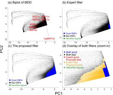
on the plane. The PCA is performed on the six QC variables to separate good SNPs from bad ones on the plane of the first two principal components (PC1 versus PC2), which usually account for about >80% of the variation in the original QC variables. The use of PCA
facilitates the task of modeling all of these QC variables that can be highly correlated. It also projects good SNPs into a concentrated corner on the plane and spreads out bad SNPs in
opposite directions along the axes of the original QC variables (e.g. see the biplots shown in Figures 1a and 2a, and the expert SNP classification in Figures 1b and 2b). Different studies may result in different patterns of PC biplots, but the key common feature is that good SNPs
Given the PCA plots, we use DBSCAN (Ester et al., 1996) to define the boundaries of the good SNPs. DBSCAN is a density-based clustering algorithm, it performs efficiently on
large-scale datasets, and most importantly, it can find clusters of arbitrary shape. Given a data space, it defines regions of high-density points as clusters and classifies regions of low-density points as noises (i.e. a noise is a point that does not belong to any clusters). DBSCAN
requires that for each point in a cluster, there are at least a minimum number, K, of points in the neighborhood of a given radius r of the target point. Ester et al. recommended setting K
to four, and to determine r from the data via the following steps. First, calculate the distance of each target point to its K-th nearest point. Next, plot the sorted K-th nearest neighbor (NN) distance (which is referred to as the sorted K-th NN graph). Finally, set r to the Y-axis value
where a sharp jump occurs. We follow the suggestion of using K =4. Instead of eyeballing the value for r as suggested by the original work, we solve for r by fitting a change point
model as described in the Appendix A1. The r value determined by the change-point method should be viewed as an initial value, and should be further fine tuned until certain criteria are fulfilled. For example, tune r until the resulting ‘good’ SNPs yield a desirable λ value (i.e. the
inflation factor of the test statistics; Devlin and Roeder, 1999), until maximum MSP is smaller than a desirable level, or until a certain percentage of SNPs are removed. With the
suitable r value, we then use the largest cluster identified by DBSCAN to define the boundaries for good SNPs (e.g. see the borders of the blue area in Figures 1c and 2c). The boundaries represent meaningful thresholds with respect to the original QC variables. In the
Criterion (ii) ensures the monotonicity of the thresholding. That is, any SNPs located in the ‘good SNP corner’ (i.e. high logMAF, low MSP and low MSP/MAF) will be included even if
they are not dense enough to be included in a cluster.
Performance evaluations using real datasets. The performance of the proposed QC algorithm was evaluated using the seven GWAS studies conducted by WTCCC, including
bipolar disorder (BD), coronary artery disease (CAD), CD, hypertension (HT), rheumatoid arthritis (RA), Type 1 diabetes (T1D), and T2D (WTCCC, 2007). In addition, we also assess
the algorithm using the MDD dataset from GAIN studies (Sullivan et al., 2009). In each WTCCC GWAS, there were 490 032 SNPs genotyped on chromosomes 1 to 22 from 2000 cases and 3000 common controls, which included 1500 from the 1958 British Birth Cohort
(58C) and another 1500 from blood donors recruited by UK Blood Services. We excluded unreliable individuals as defined in the original studies: poor sample call rate (<97%),
extreme overall heterozygosity (>30% or <23%) and high genome-wide IBD values (>0.86), and obtained on average 1887 cases and 2974 controls. We then removed those SNPs with HWE P-value < 5.7×10⁻⁷ (WTCCC, 2007) and were left with 474 657 SNPs for the QC
evaluations. The MDD study contained 556 131 SNPs genotyped on chromosomes 1 to 22 from 1738 MDD cases and 1802 controls. In this dataset, all unreliable samples (e.g. poor
sample call rate, extreme heterozygosity, high relatedness and ancestral outliers) have been excluded using the steps described in Sullivan et al. (2009). We removed SNPs with HWE P-value < 5.7×10⁻⁷ and performed the QC analysis on the remaining 526 740 SNPs.
1% if MAF < 5% or SNPs with MAF ≤ 1%. The performances are assessed based on the following four criteria: (i) percentage of SNPs excluded due to low quality; (ii) inflation
factor of the substructure-adjusted test statistics λ; (iii) number of false associations found in the filtered dataset [referred to as false positives (FP)]; and (iv) number of true associations missed in the filtered dataset [referred to as true positives (TP)]. For (ii), the inflation factor λ
is calculated as the median of the observed test statistics of association divided by the median of χ2(1) distribution (i.e. 0.456) (Devlin and Roeder, 1999). For the WTCCC datasets, the
association statistics were calculated using a stratified Cochran– Mantel–Haenszel test in PLINK (Purcell et al., 2007) to adjust for population substructure. For the MDD dataset, the trend test statistics were used because the samples are ancestrally homogeneous (Sullivan et
al. 2009). For (iii), an FP is defined as a significant signal found in the data analyses but not confirmed in the literature (i.e. neither in PubMed database nor the published GWAS catalog
at www.genome.gov/gwastudies). For (iv), a TP is defined as a significant signal found in the data analyses and also confirmed in the literature (either in PubMed or the published GWAS catalog). A P-value threshold of 5×10⁻⁷ (following the WTCCC paper) is used to define
significance. However, because there were no literature-confirmed signals that survived the 5×10⁻⁷ threshold for BD, HT and MDD, we used a less stringent threshold of 10−5 for the
P-value in our analysis for these three diseases. A threshold of 10−5 is considered to be a moderate association in the WTCCC studies (WTCCC, 2007).
R and runs DBSCAN using C++ code written by us for speed improvement. The software and instructions are available for download from the corresponding author’s website.
Results
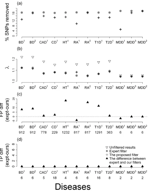
Figure 3 shows the results of our method and the WTCCC expert filter based on the four criteria. The specific numerical results are given in the Supplementary Tables 1 and 2.
To illustrate, we report the results using the r value obtained by the change-point model for all eight diseases regardless of whether a further fine-tuning of r was carried out. Overall, the
algorithm with change-point r removed from 2.8% to 14.6% fewer SNPs than the expert filters, and yet had either smaller or comparable λ values, contained fewer or comparable FPs, and retained the same TPs (which were all the TPs in the genotyped SNPs). The
maximum MSP retained in the datasets ranged from 4.44% to 5.55% for the WTCCC datasets and was 37.63% for MDD.
Carefully examining Supplementary Tables 1 and 2, we saw that there were three diseases where the performance with the initial change-point r value was not as good as expert filters in some of the criteria: BD (having a larger λ=1.123 than the 1.122 of the expert
filter), RA (having a larger λ=1.083 than 1.052 of expert and including four more FPs) and MDD (having two more FPs than expert). Using BD as an example, with the change-point r
value, our filter removed 13.2% of the SNPs (versus 18.6% of expert), and the resulting ‘good’ SNPs had a maximum MSP of 4.91%, a not small λ value of 1.123 (versus 1.122 of expert), 19 FPs (versus 27 of expert, out of 912 unfiltered FPs) and retained all 6 TPs (same
that the two filters removed about the same proportion of SNPs. With a similar removal rate (18.2% versus 18.6% of expert), our algorithm gave a slightly smaller λ (1.114 versus 1.122)
and kept fewer FPs (18 versus 27). The results of the TPs remained unchanged.
In RA, we removed 9.8% of SNPs (versus 18.7% of expert), which resulted in a maximum MSP of 5.55%, a λ of 1.083 (versus 1.052 of expert), 211 FPs (versus 207 of
expert, out of 817 unfiltered FPs), and the same number of TPs as the expert filter (6 out of 6 unfiltered TPs). When we removed about the same proportion of SNPs as the expert filter
(18.5% versus 18.7%), the remaining good SNPs yielded a slightly smaller λ (1.048 versus 1.052), contained 16 fewer FPs (191 versus 207) and the same number of TPs (6). In MDD, with the change-point r, the algorithm removed much fewer SNPs (5.26% versus 19.89%),
yielded comparable λ (1.043 versus 1.044), but kept two more FPs (6 versus 4 out of 6 unfiltered FPs) compared to the expert filter. Because the resulting maximum MSP was too
large (i.e. 37.6%) when we used the change-point r, we tuned r by decreasing its value till the maximum MSP was <10% (i.e. 9.7%). The λ and FPs became 1.044 and 4, respectively, which were the same as the expert filters. The λ and FPs stayed unchanged when we
continued tuning r until we had removed the same proportion of SNPs as the expert filter. We also categorized the SNPs into four groups according to whether they were
included (i.e. labeled as ‘good SNP’) or excluded (i.e. labeled as ‘bad SNP’) by our filter and the expert filter (Table 1). For all of the diseases, our algorithm and the expert filter have around 80% agreement in inclusion and around 12% agreement in exclusion on average. The
expert filter, and the overlay of the two on a two-dimensional PC plane using CAD (Figure 1d) and MDD (Figure 2d) (see Supplementary Figure 1 for other diseases). Instead of the
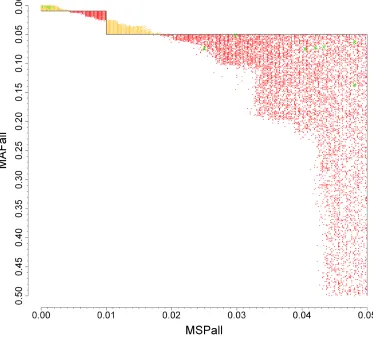
step-like boundary of good SNPs in the expert filter, our filter gives a smoother boundary of good SNPs. Figure 4 further illustrates the disagreements on the axes of MSP versus MAF (instead of PC1 versus PC2) for CAD (see Supplementary Figure 2 for other diseases). The
yellow dots represent SNPs that are labeled as ‘good’ by our algorithm but ‘bad’ by expert filters. One group of yellow dots occurred in the extremely low MAF and low MSP range,
indicating that our algorithm would keep SNPs of MAF < 0.01 when their MSPs were extremely low. In contrast, the red dots represent the SNPs that are labeled as ‘bad’ by our algorithm but ‘good’ by expert filters. The big red area on the right side indicates that our
algorithm gives a more stringent MSP criterion for good SNPs than the expert filter (i.e. MSP < 5%): our criteria ranged from MSP < 2% to MSP < 4%, depending on the MAF. Lastly, the
two red and yellow triangles in the upper middle area show the impact of the ‘smoother’ threshold of our algorithm: it has a more stringent MSP threshold when MAF is 0.01–0.025, and a less stringent threshold when MAF is 0.025–0.05.
Discussion
Ensuring the quality of genotype data is essential for drawing accurate and replicable
conclusions (Donnelly, 2008). In this work, we have introduced a QC algorithm to identify SNPs with low QC features using criteria determined through PCA and DBSCAN. The proposed filter is in essence an ‘unsupervised’ (i.e. algorithm determined) version of the
PCA to jointly model the potentially highly correlated QC variables, and use DBSCAN to identify the borders of good-SNP clusters that have arbitrary shapes. The boundary of the
good-SNP cluster can be translated directly to meaningful thresholds for the original QC variables. The proposed algorithm retains the rationale of the expert filter to identify QC outliers, avoids arbitrary decisions on cutoff values and gives contingent MSP thresholds for
different MAF values. The data applications show that with the same or fewer SNPs discarded due to bad quality, the proposed algorithm has comparable or better performance
than the expert filter for all diseases.
The underlying rationale of our algorithm is that the majority of genotyped markers have sufficient genotyping quality, and hence low-quality SNPs can be treated as outliers and
be identified by looking for SNPs with distinct QC features. To facilitate the implementation of the idea, we use PCA on the original QC variables. PCA consolidates the information
from the many correlated QC variables, and projects SNPs onto a two-dimensional PC plane where good SNPs clump together into a corner of desirable QC values, whereas bad SNPs fan out in all directions. It is expected that the PC biplot may differ from one study to
another: in our exploration, we have seen different patterns in the biplots for WTCCC datasets and for the MDD dataset. Yet all biplots have good SNPs lumped into a corner that
corresponds to good QC features.
We wish to point out that when using the proposed algorithm, it is important to monitor the features of the retained good SNPs and tune the neighborhood radius r to
proportion of data points are of low quality. For example, in the MDD dataset, there were about 11.4% of SNPs with MSP > 10%, and our algorithm with the initial change-point r
kept SNPs with MSP up to almost 38%. Tuning of r was thus continued until the maximum MSP dropped to < 10%. In practice, the smaller r is, the more stringent the QC criteria for ‘good’ SNPs will be, as a smaller r makes it harder to form a cluster in DBSCAN. We
suggest starting with a value of r determined by fitting a change-point model to the sorted fourth nearest distances, and then further to adjust r until the specific goal is reached, so as to
assure the λ value, the maximum MSP, or the percentage of SNPs removed within reasonable ranges. In our explorations, we found that the change-point r often suggests a reasonable value (e.g. in CAD, CD, HT, T1D and T2D) or is at least a good upper bound (e.g. in BD,
RA and MDD, judging by the resulting λ values or the retained maximum MSP). Given the change-point r, one can reduce its value if a more stringent filter is needed, and increase its
value if one wishes to remove only extreme outlier SNPs.
When selecting which QC variables to include in the algorithm, we intend to avoid using MAFcs and MAFcn because they may obfuscate the true associations. For the rest of
the QC variables, it is possible to make other choices for inclusion/exclusion, e.g. to exclude MSPall from the proposed QC variable set (i.e. to use five variables), or to include
MSPall/MAFall to the proposed QC variable set (i.e. to use seven variables). While we expected that the performance would not change much, we carried out sensitivity analyses to evaluate the impact of using different QC variables in the proposed algorithm. The results are
expected, the 7- and 5-variable analyses performed very similarly to the proposed 6-variable analyses, indicating the robustness of the proposed filter to the different choices of QC