2152 | P a g e
Mutli-Objective Optimisation of Process Parameters in
Statistical Relations Support ACO seed MFSA Method of
Milling Operations Process on AL 6063-T6
Dr.D.Ramalingam*
1, R.Rinu Kaarthikeyen
2, Dr.S.Muthu
3, Dr.V.Sankar
4*
1Associate Professor, Nehru Institute of Technology, Coimbatore, (India)
2Research Associate, Manager – Engineering, TCMPFL, Chennai, (India)
3
Principal, Adithya Institute of Technology, Coimbatore, (India)
4
Professor, Nehru Institute of Engineering and Technology, Coimbatore, (India)
ABSTRACT
Milling process is one of the well accepted applications process in manufacturing as extensive and precision
operations among all machining methods. During this operation the very common issues are being faced by
every manufacturer like attaining the dimensional accuracy and precision, required surface finish. With the
objective of achieving the desired surface finish and minimum tool wear the optimization while milling Al 6063
– T6 material through accepted set of optimisation algorithms application in MATLAB programming this
attempt is chosen. On identifying the best converged algorithm, subsequently the regression equations are
incorporated in the programme as the initiation to predict the combination of optimised parameters in line with
the defined objective and the simulation continued. The optimised parameter combinations were identified for
each output parameter (Surface roughness and Tool flank wear).
Key words- Milling, Al6063-T6, Regression, Ant Colony Algorithm, Cuckoo Search, Genetic
Algorithm, Modified Fish Swarm Algorithm, Particle Swarm Optimization Algorithm, Scatter
Search Algorithm, Optimization, Minitab, MATLAB.
I. INTRODUCTION
2153 | P a g e
Inconsistency in the end surface quality of the produced parts also influenced through tool cutting edges stability which is the indication of tool flank wear. In turn the tools wear leads for the increase in cost of production and down time. As the selection of optimal cutting conditions and cutting parameters and machining environment is a prime call for any machining operations, this effort is taken with the aim on the multi-objective optimisation of process parameters cutting speed, depth of cut, feed, and cutting fluid flow rate in milling process of Al6063-T6 material.
Abbreviations Used
DOC Depth of cut R-sq (adj) R - square adjusted statistical value Exp Experiment R-sq (pred) R - square predicted statistical value F Feed rate S Cutting speed
FF Fluid Flow rate GA Genetic Algorithm FW Tool Flank Wear SSA Scatter Search Algorithm MMC Metal matrix composite CSA Cuckoo Search algorithm Ra Surface roughness MFSA Modified Fish Swarm Algorithm Reg Regression PSO Particle Swarm Optimization R-sq R - square statistical value ACO Ant Colony Algorithm
II. LITERATURE SURVEY
With the nonstop efforts put in by many researchers in making attempts through quite a lot of methods and skill to address the issues related and suggesting varieties in approaches to achieve the expected level of results in various machining processes on various materials like metals, alloys, composites. In addition, to identify and resolve the effects of input machining parameters on the output parameters almost all many of the researchers used optimization techniques. Tsao, C C [1] through the experimental investigation has proved the adaptability of Grey - Taguchi method in optimization of the parameters in milling operations on the aluminium alloy and predicted that the grey-Taguchi method is suitable for solving the surface finish quality and tool flank wear. Raviraj Shetty et al. [2] demonstrated by an exclusive study with the Taguchi optimization method for optimizing the process parameters in the turning operation on the age hardened AlSiC - MMC with CBN cutting tool. Paulo Davim, J [3] indicated that the higher cutting speed results in a smoother surface, through the application of Taguchi method in the experimental investigation conducted. Wang et al. [4] executed an experiment and optimized the machining variables involved for estimating and confirming the economic machining conditions in turning process by a deterministic approach.
David et al. [5] have predicted that the surface quality in high speed end-milling process by ANN approach and statistical tools towards different surface roughness predictor’s combinations. In addition, Kirby, D.E, and
2154 | P a g e
on GFRP composite material than the solid carbide end mill. Godfrey et al. [8] devised a novel model for correlating the relationships of drilling parameters and the effects on axial force and torque acting on the cutting tool by means of RSM approach. They have concluded that the torque varies non-linearly with reference to the chief cutting parameters like speed, feed rate, and diameter. Singh et al [9] have attempted in correlating the drilling-induced damage with the drilling parameters on UD-GFRP laminates.
III. EXECUTED EXPERIMENT AND OBSERVED DATA
K. Sundara Murthy and I. Rajendran, [10] executed an end milling operations experiment on the AL6063-T6 material specimen with the dimensions of 300 x 200 x 50 mm in the 3 HP powered universal geared type milling machine. The mechanical properties of the experimented material is with of Hardness (Brinell) - 73; Ultimate Tensile Strength - 241MPa; Tensile Yield Strength- 214 Mpa; Elongation – 12 %; Modulus of rigidity 68.9 - GPa; Fatigue strength – 68.9 GPa; Shear modulus – 25.8 GPa; Shear Strength – 152 MPa and Poisson’s ration- 0.33. LT740WWL category end mill cutting tool of 20 mm diameter with coated inserts APGT 1003 PDER-Alu LT05 are chosen to perform the operations. Vegetable oil coolube 2210 was applied as the cutting fluid in the process with MQL setup. The input machining variables chosen for the process in three states as noted in the Table 3.1. The output parameters taken for analysis were the surface roughness and flank wear of cutting tool which were measured through tool room microscope and surface roughness tester. The experimental observed data through Taguchi L9 array experimental plan are given in the Table 3.3, where S stands for cutting speed in m / min; F is feed in mm / min; DOC is depth of cut in mm / min; FF is fluid flow rate in ml / hr; Ra is surface roughness in µm and FW represents the tool flank wear in mm.
Table 3.1 Machining parameters and levels
Parameters State 1 State 2 State 3
S, Cutting speed, m / min 35 56 88
F, Feed velocity, mm / min 180 250 355
DOC, Depth of cut, mm / min 1 1.2 1.4
FF, Fluid flow rate, ml / hr 300 600 900
Table 3.2 Experimental observed
Exp No S F DOC FF Ra FW
1 35 180 1.0 300 0.799 0.256
2 35 250 1.2 600 0.746 0.240
3 35 355 1.4 900 0.973 0.274
4 56 180 1.2 900 0.752 0.202
5 56 250 1.0 300 0.868 0.329
6 56 355 1.4 600 0.449 0.370
7 88 180 1.4 600 0.649 0.316
8 88 250 1.0 900 0.678 0.383
9 88 355 1.2 300 0.747 0.395
2155 | P a g e
conclusion projected is that the optimal parameters combination - cutting speed of 88 m / min, feed velocity of 180 mm / min, depth of cut of 1.4 mm and coolant flow rate of 600 ml / hr.
IV. MATHEMATICAL MODELING
To access the influence of the input variables (Cutting speed, Tool Feed, Depth of cut and Cutting fluid flow rate) on the output variables (Surface roughness and Tool flank wear) through the regression analysis Minitab17 software is used. Since the R - sq values are better in second order equations than the first order which indicates that the predictors explain about 99.91% of the variance in the output variables, also the adjusted R - sq values are close to the R - sq values which accounts for the number of predictors in the regression model and reveals the model fits significantly. In the way, such framed second order regression equations through the Minitab17 for the individual output parameter in terms of input parameter combination are
Ra = (2.187) + (0.00965 x S) – (0.010475 x F) – (0.945 x DOC) – (0.000085 x FF) + (0.000010 x S x F) – (0.01042 x S x DOC) + (0.007964 x F x DOC) (4.1)
“FW = -(0.363) + (0.01709 x S) + (0.001596 x F) + (0.171 x DOC) – (0.000224 x FF) – (0.000025 x S x F) –
(0.00700 x S x DOC)+ (0.000182 x F x DOC) (4.2)
Speed is contributing the highest significance (47.5%) on the results which is followed by feed (29.6%) as an individual predictor. Two predictors model is concern with the lowest Cp value (4.2), highest adjusted R-sq value (69.5) and low S value (0.037688) is for the speed and feed combination. In the case of three predictors model the combination of Speed, feed and fluid flow records the significance contribution. The Doc is the least contributing predictor on the outcome.
V. OPTIMIZATION METHODOLOGIES ADOPTED
The objective functions taken for the optimization to obtain minimum surface roughness and minimum tool
flank wear. Analysis to optimise and predict the outcome are executed by applying
Ant Colony Algorithm,
Cuckoo Search, Genetic Algorithm, Modified Fish Swarm Algorithm, Particle Swarm Optimization
Algorithm, Scatter Search Algorithm
in the MATLAB programming with Elman Back Propagation. The experimental data set are given initially to train the programme with random selection of parameter values and compiled with 5000 iterations. The performance of the simulation referring with MSE values of each algorithm is evaluated. It has been noted that Modified Fish Swarm Algorithm converges as the best with minimum mean error in simulation followed by the ACO, PSO, SSA, CSA, GA respectively as listed in the Table 5.1. With an idea of feeding the simulated outcome of the second best fit algorithm (ACO) to the first best fit algorithm (MFSA) as the initial parameters set and the procedure of simulation carried out. Hybridization of regression relationship equations as the condition for simulation is also put in effect.2156 | P a g e
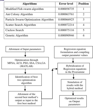
Algorithms Error level Position
Modified Fish swarm algorithm 0.000058735 1
Ant Colony Algorithm 0.000063761 2
Particle Swarm Optimization Algorithm 0.000066925 3 Scatter Search Algorithm 0.000072214 4
Cuckoo Search 0.000075116 5 Genetic Algorithm 0.000090946 6
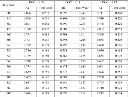
Figure 5.1 Block diagram of hybridization
As this effort yields improved state of results, for projecting the results with smooth curve fittings the input parameters level are subdivided into equal parts into steps as given in the Table 5.2.
Table 5.2 Step values allotment of input variables
Sl No Parameter Initial Value Step value Final value
1 Cutting speed (m / min) 35 3.533333 88 2 Feed velocity (mm / min) 180 11.666667 355 3 Depth of cut (mm) 1.0 0.026666 1.4 4 Fluid flow rate (ml / hr) 300 40 900
Table 5.3 Simulated results of v = 35; f = 180 (DOC 1.00, 1.03, 1.05)
fluid flow DOC = 1.00 DOC = 1.03 DOC = 1.05 Ra Tool Wear Ra Tool Wear Ra Tool Wear
300 0.799 0.256 0.803 0.252 0.804 0.252 340 0.687 0.256 0.798 0.274 0.803 0.278
380 0.882 0.238 0.796 0.236 0.796 0.232
Allotment of Input parameters
Optimization through MFSA, ACO, PSO, SSA, CSA,GA
(MATLAB)
Regression equation formulation and compiling
output parameter values
Identification of best two optimization
algorithm
Hybridization of Regression equations
in the Programme
Simulation of results with the
hybrid method
Optimized results on Output parameters Allotment of the
second best method’s output as input to the
2157 | P a g e
420 0.789 0.247 0.793 0.227 0.794 0.224 460 0.784 0.220 0.788 0.216 0.790 0.215
500 0.781 0.240 0.783 0.206 0.788 0.208
540 0.775 0.201 0.782 0.200 0.784 0.200 580 0.774 0.194 0.776 0.189 0.783 0.191
620 0.773 0.184 0.774 0.180 0.780 0.181 660 0.767 0.174 0.770 0.172 0.776 0.171
700 0.763 0.166 0.767 0.163 0.773 0.164
740 0.761 0.156 0.765 0.153 0.769 0.154 780 0.758 0.146 0.759 0.148 0.764 0.142
820 0.752 0.138 0.756 0.134 0.762 0.133
860 0.750 0.127 0.753 0.126 0.652 0.128 900 0.745 0.118 0.751 0.116 0.656 0.116
Table 5.4 Simulated results of v = 35; f = 180 (DOC 1.08, 1.11, 1.13)
fluid flow
DOC = 1.08 DOC = 1.11 DOC = 1.13
Ra Tool Wear Ra Tool Wear Ra Tool Wear
300 0.806 0.253 0.692 0.249 0.711 0.248 340 0.806 0.274 0.808 0.266 0.810 0.256
380 0.801 0.232 0.690 0.233 0.706 0.228 420 0.798 0.222 0.801 0.222 0.803 0.253
460 0.794 0.215 0.798 0.214 0.800 0.214
500 0.791 0.205 0.794 0.206 0.685 0.205 540 0.789 0.199 0.793 0.198 0.678 0.196
580 0.786 0.188 0.788 0.185 0.676 0.183
620 0.779 0.180 0.782 0.178 0.685 0.179 660 0.778 0.169 0.670 0.170 0.687 0.165
700 0.774 0.159 0.673 0.160 0.691 0.158 740 0.659 0.153 0.677 0.149 0.696 0.151
780 0.663 0.142 0.681 0.142 0.700 0.139
820 0.667 0.132 0.686 0.132 0.705 0.135 860 0.671 0.123 0.691 0.122 0.710 0.125
900 0.676 0.119 0.695 0.118 0.715 0.114
2158 | P a g e
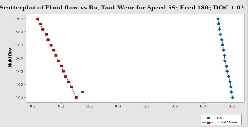
depicts the results for the DOC 1.08 mm / min to 1.13 mm / min. Fig. 5.2 to 5.7 represents the curve fit in for the simulated results.
Figure 5.2 Fluid Flow Vs Ra, Tool wear for Speed 35, Feed 180, DOC 1.0
2159 | P a g e
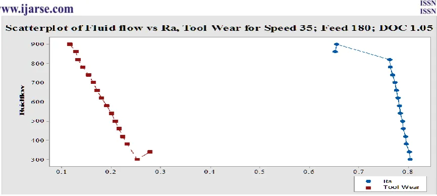
Figure 5.4 Fluid Flow Vs Ra, Tool wear for Speed 35, Feed 180, DOC 1.05Figure 5.5 Fluid Flow Vs Ra, Tool wear for Speed 35, Feed 180, DOC 1.08
2160 | P a g e
Figure 5.7 Fluid Flow Vs Ra, Tool wear for Speed 35, Feed 180, DOC 1.136 RESULTS AND CONCLUSIONS
Speed is contributing the highest significance (47.5%) on the results which is followed by feed (29.6%) as an individual predictor. Two predictors model is concern with the lowest Cp value (4.2), highest adjusted R-sq value (69.5) and low S value (0.037688) is for the speed and feed combination. Modified Fish Swarm Algorithm converges as the best with minimum mean error in simulation followed by the ACO, PSO, SSA, CSA, GA respectively.
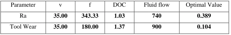
Table 6.1 Optimized parameter combination for Surface roughness and Tool wear
Parameter v f DOC Fluid flow Optimal Value
Ra 35.00 343.33 1.03 740 0.389
Tool Wear 35.00 180.00 1.37 900 0.104
The proposed regression relationship coupled ACO feed MFSA algorithm model has the conformity with investigational values, with mean value error of 0.00006 and this multi objective optimization approach is capable of predicting the optimum machining parameters combination in end milling operations of the tested Aluminium 6063 T6 material. The fit in curves may be used as the reference to the manufacturers at time of processing. The regression relationship equations may be taken as the input phenomenon for simulation only after the confirmation of the statistical significance.
REFERENCES
[1] C C. Tsao, Grey - Taguchi method to optimize the milling parameters of aluminum alloy, Int. J. Adv. Mfg. Tech, 40, 2009, 41-48.
[2] Raviraj shetty, Taguchi’s techniques in machining of metal matrix composites. J. of the Braz .society of
2161 | P a g e
[3] J. Paulo Davim, A note on the determination of optimal cutting conditions for surface finish obtained inturning using design of experiments, J Mater Process Technol, 116, 2001, 305-308.
[4] J.Wang, T.Kuriyagawa, X P. Wei and D M. Guo, Optimization of cutting condition for single pass turning operation using a deterministic approach, Int. J. Mach. Tools Manuf, 42, 2002, 1023-1033.
[5] V. David, M. Ruben, C. Menendez, J. Rodriguez and R. Alique, Neural networks and statistical based models for surface roughness prediction, International Association of Science and Technology for Development. Proceedings of the 25th IASTED international conference on Modeling, Identification and Control, 2006, 326-331.
[6] D E. Kirby and C C. Joseph, Development of a Fuzzy-Nets-Based surface roughness prediction system in turning operations, Journal of Computers & Industrial Engineering. 53, 2007, 30-42.
[7] Praveen Raj, P., Elaya Perumal, A. 2010. Taguchi Analysis of surface roughness and delamination associated with various cemented carbide K10 end mills in milling of GFRP. Journal of Engineering Science and Technology Review, 3, pp. 58-64.
[8] Godfrey, C., Onwubolu, Shivendra Kumar 2006. Response surface methodology-based approach to CNC drilling operations. Journal of Materials Processing Technology, Vol. 171, pp. 41–47
[9] Singh, I., Bhatnagar, N. 2006. Drilling of uni-directional glass fibre reinforced plastic (UD-GFRP) composite laminates. International Journal of Advanced Manufacturing Technology, Vol. 27, pp. 870–876