_____________________________________________________________________________________________________ *Corresponding author: E-mail: [email protected];
www.sciencedomain.org
Development of a Potentially Individualized
Algorithm to Detect Heart Failure Events through
Home Telemonitoring
Kiswendsida Sawadogo
1*, Jérôme Ambroise
1, Steven Vercauteren
2,
Michel Vanhalewyn
3, Marc Castadot
2, Jacques Col
2and Annie Robert
11
The Pôle de Recherche Epidémiologie et Biostatistique, Institut de Recherche Expérimentale et Clinique (IREC-EPID), Université Catholique de Louvain, Clos Chapelle-aux-champs 30, box B1.30.13 1200 Brussels, Belgium. 2
The Brussels Heart Centre (BHC), Clinique Saint Jean, Boulevard du Jardin Botanique 32, 1000 Brussels, Belgium. 3
Société Scientifique de Médecine Générale (SSMG), Rue de Suisse 8, 1060 Brussels, Belgium.
Authors’ contributions
This work was carried out in collaboration between all authors. Author KS performed data analysis and drafted the manuscript. Author JA took part in data analysis and in drafting the paper. Authors SV, MV, MC, JC and AR participated in the design and the study protocol implementation. Author JC also contributed to writing the paper. Author AR also supervised the study. All authors read and approved the final manuscript.
Article Information
DOI: 10.9734/BJMMR/2017/29098 Editor(s): (1) Bertram Pitt, Division of Cardiology, University of Michigan School of Medicine, Ann Arbor, MI, USA. (2)Nurhan Cucer, Erciyes University, Medical Biology Department, Turkey. Reviewers: (1) Jerzy Bełtowski, Medical University, Poland. (2)Maddury Jyotsna, Deemed University, India. (3)Rui Xiang, Columbia University, USA. Complete Peer review History:http://www.sciencedomain.org/review-history/17118
Received 22nd August 2016 Accepted 25th November 2016 Published 3rd December 2016
ABSTRACT
Aims: Home telemonitoring represents a promising approach to reduce heart failure (HF) patients’ hospital readmissions. The aim of the study was, in a first step, to identify the monitored parameters’ characteristics that are predictive of HF events. In a second step, it was to build a prediction score by combining both the identified characteristics and the patients’ clinical prognosis.
Methods: Patients completed 6-month blind daily body weight, blood pressure and pulse
measurements. A cardiac composite endpoint (CCE) of death, hospitalization or urgent visit was considered. A series of signal-derived statistics (SDS) were computed on 3, 5 and 7 days’ time windows. A signal score for CCE prediction was built by including SDS in a first logistic model using a subset of signal set (training) and its accuracy was assessed in another subset (testing). A clinical score was computed using the Meta-Analysis Global Group in Chronic Heart Failure formula. Both scores were combined using a second logistic model. We compared the three scores using ROC curves.
Results: Monitoring was completed by 146 patients and 96 CCE occurred in 61 patients. The first logistic model resulted in a signal score which combined 7 SDS including body weight’s variability on 3 consecutive days, body weight’s increase on 3 and 7 consecutive days, pulse’s variability on 3 and 7 consecutive days, diastolic blood pressure’s mean on 3 consecutive days, differential pressure’s variability on 3 consecutive days. The signal score had ability in predicting CCE occurrence (training set: AUC= 0.796, P < .001; testing set: AUC=0.830, P < .001). The second logistic model resulted in a combined score that improved CCE prediction (training set: AUC= 0.830, P < .001; testing set: AUC= 0.891, P < .001) with 92% sensitivity and 77% specificity. Conclusions: Signal data and clinical data provide additive information to risk prediction.
Keywords: Heart failure; telemonitoring; hospital admission; prediction.
1. INTRODUCTION
Heart failure (HF) is the leading cause of hospitalization in people older than 65 years [1]. These patients then frequently experience repeated hospitalizations or urgent visits to a medical specialist or even death. In Western Europe, hospital readmission rate reached 24% within 12 weeks of HF discharge [2]. These events should be predicted. Several studies [3-5] suggested to remotely monitor clinical parameters with detectable changes such as body weight, blood pressure or pulse rate, for early detection of HF events. However, the clinical efficacy of technology-assisted remote home telemonitoring (HTM) remains debated [6]. The European Society of Cardiology (ESC) recommends that a patient with a body weight increase of 2 kg or more in 3 days, alerts a healthcare professional for early pharmacological intervention [7]. This standard rule has been assessed in the WISH trial which showed no reduction of death or HF-related hospitalizations in the HTM group [3]. Two major multicenter randomised controlled trials (RCTs) assessed other published simple decisions rules (body weight > 3 lbs in 1 day or > 5 lbs in 3 days) and failed to demonstrate superiority of HTM protocols over usual care [8,9]. Even the recent BEAT-HF trial, one of the largest RCTs of remote HTM in an HF population showed no significant effect of HTM in reducing hospital readmission rate [4]. However, meta-analyzes which include these RCTs continue to suggest a significant effect of HTM in reducing HF-related events [5,10]. The main constraint is that there is no consensus on the threshold of change in these clinical parameters, or on the corresponding time
window that should lead to trigger an alert. To improve the diagnostic power of HTM algorithms in detecting HF events, the characterization of clinical parameters’ changes that are associated with HF events is a prerequisite. Subsequently, the development of a potentially individualized algorithm could provide a better performance in predicting HF events [11]. The aim of the present study, part of the Better Efficacy in Lowering events by General practitioner’s Intervention Using remote Monitoring in Heart Failure (BELGIUM-HF) project was to find a better measurement through HTM parameters to better predict HF events. It was in a first step, to identify characteristics in the dynamic (daily changes) of the monitored parameters (body weight, blood pressure, pulse rate) that are predictive of HF events. In a second step, it was to build a potentially individualized prediction score using both the identified characteristics and the patients’ clinical prognosis as estimated by the clinical score developed by the Meta-analysis Global Group in Chronic Heart Failure (MAGGIC) [12].
2. METHODS
2.1 Patients
protocol conforms to the ethical guidelines of the 1975 Declaration of Helsinki.
2.2 Study Outcomes
The predictive performance of HTM was developed with respect to the occurrence during 6-months of follow-up of a cardiac composite endpoint (CCE). CCE was defined as death or hospitalization or a non-scheduled call from the patient leading to an urgent visit of the physician and resulting in a medical intervention such as a change in diuretics doses. Events were classified as cardiac or non-cardiac events due to co-morbidities. Death was assumed being cardiac unless an immediate non-cardiovascular cause was clearly documented.
2.3 Signal Acquisition
HF is accompanied by several changes induced by various mechanisms including an activation of neuro-humoral reflexes resulting in detectable changes in water retention which may precede the clinical deterioration [14]. An increased global sympathetic activity also accompanies HF producing detectable changes in heart rate, rhythm, systemic and pulmonary pressures [14]. Therefore, it seemed relevant to remotely monitor patients’ body weight, blood pressure and pulse rate.
In this study, we used an automatic non-invasive monitoring with home-based portable technology. Patients were provided with Bluetooth-coded sphygmomanometers and scales (Vitalsys Inc) and dedicated mobile phones (Belgacom Inc). The equipment was hiding all results of daily measurements of blood pressure, pulse and
body weight. An auditory signal informed patient when data were transmitted. No additional messages were programmed. A nurse-technician visited each patient, installed the material in an adequate space and taught him the procedure. He instructed the patient to make measurements each morning after having emptied the bladder and before breakfast. He also called the patient when more than 2 days elapsed without measurements and provided home assistance. Data were stored in real time at the Monitoring Data Centre (Touring Inc, Brussels). GPs were not involved in the telemonitoring procedure itself, nor were they aware of the accumulated data.
2.4 Signal Analysis and Construction of a Signal Score
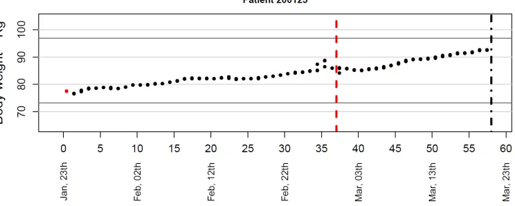
A complete signal of daily monitored parameters was available for patients who completed the study. Such a patient signal is illustrated on Fig. 1 for daily body weight’s measurements.
Each dot represents the patient daily body weight’s measurement during his follow-up between January 25th and March 21th. That patient was hospitalized on February 29th (vertical dotted line) and he died on March 21th (vertical dotdash line).
From the complete signal of each patient, a series of signal-derived statistics (SDS) were computed on a short 3 days’ time window [15,16] and a long 7 days’ time window [17] as previously used in literature, as well as on a middle 5 days’ time window. These SDS included means and standard deviations of all monitored parameters, computed based on their 3, 5 or 7
consecutive values preceding each time-point. In addition, we computed a body weight’s slope corresponding to the slope of the linear regression of body weight against measure date using the 3, 5 or 7 consecutive values of body weight preceding each time-point.
A mathematical model for CCE prediction was built in a subset of signal set (training) and its accuracy was assessed in another subset of signal set (testing). Considering that both training and testing sets had to include positive (i.e. a point with a CCE) and negative (i.e. a time-point without CCE) cases, the following procedure was applied to build these two sets. In the training set, the positive cases were included as the first event for patients with at least one CCE while the negative cases were included as a randomly selected time-point for patients without CEE. In the testing set, the positive cases were included as the second event for patients with at least two CCE while the negative cases were included as a randomly selected time-point for patients without CEE. These two sets were mutually exclusive and the same SDS were computed in both sets.
In a first step, all SDS from the training set were compared between positive and negative cases using Student t-test. In a second step, a signal score was built by including SDS in a first logistic regression with CCE as the outcome variable coded 1 if a CCE occurred and 0 otherwise. We used the log odds ratio as the signal score. Considering the large number of candidates covariates (p = 30 SDS) compared to the moderate number of observations (n=146), the coefficients of the logistic regression models
were estimated using the Least Absolute Shrinkage and Selection Operator (LASSO) method in order to avoid overfitting problem. In such dataset where the number of covariate is high compared to the number of observations, LASSO enable indeed to alleviate overfitting problem and to improve the overall prediction [18].
The selection of the variables was based on the predictive performance of the model, as recommended in such method [19]. The L1-norm penalty λ of the LASSO logistic regression model was indeed selected to maximize its predictive performance which was estimated using a leave-one-out cross validation in the training set. In this method, the model is developed on all the training set but one unit and a prediction is made for that single unit. This procedure is repeated for all units of the training set that is 146 times in our study. The L1-norm penalty λ was selected based on a 0.25 increment on a scale from 0.5 to 15, meaning a total number of 59 values considered for λ.
The predictive performance of the selected model was then computed on the testing set.
2.5 Computation of the Clinical MAGGIC Score
To build a potentially individualized prediction algorithm by combining HTM parameters to patients’ clinical prognosis, we required a valid prognostic model in HF patients. The MAGGIC group established a valid risk score of mortality in patients with HF as following [12]:
ܯܣܩܩܫܥ ݏܿݎ݁ =
+ 0.143 ∗ ቀୟୣ
ଵቁ + 0.109 ∗ ݈݉ܽ݁ − 0.035 ∗ ܾ݀ݕ ݉ܽݏݏ ݅݊݀݁ݔ
+ 0.147 ∗ ݏ݉݇݁ݎ − 0.126 ∗ ቀ௦௬௦௧ ௗ ௦௦௨
ଵ ቁ
+ 0.352 ∗ ܾ݀݅ܽ݁ݐ݁ݏ + 0.343 ∗ ܻܰܪܣ ܫܫܫ + 0.521 ∗ ܻܰܪܣ ܫܸ − 0.542 ∗ ቀ௧ ௧
ହ ቁ
+ 0.206 ∗ ܿℎݎ݊݅ܿ ܾݏݐݎݑܿݐ݅ݒ݁ ݑ݈݉݊ܽݎݕ ݀݅ݏ݁ܽݏ݁ + 0.173 ∗ ܪܨ ݀ݑݎܽݐ݅݊ + 0.038 ∗ ቀ௧
ଵ ቁ − 0.274 ∗ ܾ݁ݐܽ ܾ݈ܿ݇݁ݎ
− 0.096 ∗ ܽ݊݃݅ݐ݁݊ݏ݅݊݁ ܿ݊ݒ݁ݎݐ݅݊݃ ݁݊ݖݕ݉݁ ݅݊ℎܾ݅݅ݐݎ
ݎ ܽ݊݃݅ݐ݁݊ݏ݅݊ ݎ݁ܿ݁ݐݎ ܾ݈ܿ݇݁ݎ + 0.039 ∗ ቀ
ଵቁ ∗ ቀ
௧ ௧
ହ ቁ
+ 0.012 ∗ ቀ௦௬௦௧ ௗ ௦௦௨
ଵ ቁ ∗ ቀ
௧ ௧
ହ ቁ
2.6 Computation of a Combined Clinical-signal Score
The MAGGIC score is a cross-sectional assessment of risk whereas the signal score is a dynamic event detector. So the former can be used as a baseline risk score and the latter as a short-term predictive score. In a second logistic model, we combined these two scores to estimate a new dynamic score for predicting a CCE within the next day. The outcome in this model was the occurrence of a CCE (coded 1 if a CCE occurred and 0 otherwise) and the covariates included the signal and the MAGGIC scores. The training set was used to build this combined score and its accuracy was assessed in the independent testing set.
2.7 Predictive Performance Comparison
ROC curves were used to assess the diagnostic value of the three scores (1: The signal score, 2: The MAGGIC score, 3: The combined score) in both the training and the testing sets. Being aware of the special correlation structure of data, the performance of scores was still assessed on the whole signal time-points in all patients. Whereas the training and the testing sets included both, one selected time-point for each patient, the whole signal included all time-points with corresponding SDS in all patients. So for the
whole signal, positive cases were all time-points matching an event and negative cases were all time-points not matching an event. The signal score built in the training set was also assessed in the whole set. The MAGGIC score and the combined score were also computed in the whole set.
All statistical analyses were performed using R version 3.0.3. A workflow is shown in Fig. 2.
3. RESULTS
3.1 Baseline Characteristics
From January 2008 to December 2010, 288 patients were assessed for eligibility. However, 117 were not included because of exclusion criteria or refusal. The remaining 171 patients were enrolled but a further 25 patients failed to start home measurements because of various reasons (procedural mismatches). Monitoring was initiated in 146 patients.
The 25 patients lacking monitoring were compared to monitored patients at the starting point of HTM. They were similar for all variables but BNP neuropeptides level that was higher in non-monitored patients (P =.03) (Tables 1 and 2).
Table 1. Clinical characteristics of patients used to compute the MAGGIC score
All patients Monitoring P
Valueb
Yes No
n=171 n=146 n=25
Age --years 70.0 ± 12.0 68.2 ± 12.3 71.4 ± 9.8 .22
Left ventricular ejection fraction -- % 27.6 (7.0) 27.7 (7.1) 26.8 (6.3) .55
NYHA class III-IV –no (%) 100 (58.5) 84 (57.5) 16 (64.0) .60
Creatininea – mg/dl 1.44 (1.45) 1.45 (1.44) 1.35 (1.44) .49
Diabetes -- no (%) 59 (34.5) 46 (31.6) 13 (52.0) .07
Beta blocker -- no (%) 139 (81.2) 117 (80.1) 22 (88.0) .42
Systolic blood pressure --mmHg 117 ± 18 116 ± 19 120 ±13 .31
Body Mass Index -- kg/m2 27.2 ± 4.9 27.0 ± 4.8 28.8 ± 5.5 .09
Time since diagnosis -- months 38 ± 44 36 ± 45 48 ± 55 .08
Smoker within past 12 months – no (%) 36 (21.1) 31 (21.2) 5 (20.0) .80
COPD -- no (%) 26 (15.2) 24 (16.4) 2 (8.0) .45
Men -- no (%) 125 (73.0) 108 (74.0) 17 (68.0) .53
ACE or Sartan – no (%) 161(94.2) 138 (94.5) 23(96.0) .64
MAGGIC score -- %
Mean ± SD 34 ± 15 33 ± 14 39 ± 16 .71
Median (Percentile 25 – Percentile 75) 34 (24 – 45) 34 (25 – 45) 32 (21 -44)
Minimum - Maximum 0 - 73 0 - 73 0 - 72
a
Table 2. Clinical characteristics not included in the MAGGIC score
Variables All patients Monitoring P
Valuec
Yes No
n=171 n=146 n=25
Body weight -- kg 77.9 ± 16.8 77.1 ± 16.3 82.8 ± 19.6 .12
Diastolic blood pressure -- mm Hg 71± 13 71 ± 13 73 ± 13 .48
Pulse -- beat per minute 79 ± 17 78 ± 17 82 ± 18 .28
Cardiovascular Risk Factors
Hypertension -- no (%) 98 (57.3) 82 (56.2) 16 (64.0) .52
Diabetes -- no (%) 59 (34.5) 46 (31.6) 13 (52.0) .07
Hyperlipidemia -- no (%) 88 (57.3) 74 (50.6) 14 (56.0) .67
Medical History
Ischemic Heart Disease -- no (%) 106 (61.9) 86 (58.9) 20 (80.0) .07
Alcohol Excess -- no (%) 14 (8.2) 13 (8.9) 1 (4.0) .70
Investigations
GFRa -- ml /min/ 1.73m2 57 ± 21 57 ± 20 54 ± 19 .49
BNPb-- pg/mL IQR
814 (339; 1846)
781 (291; 1754)
1230 (283; 4470)
.03
NTerminal-Pro BNPc -- pg/mL IQR
3896 (1998; 6890)
3813 (1854; 6894)
4882 (3105; 6595)
.45
Concomitant Treatment
Loop Diuretics -- no (%) 169 (98.8) 145 (99.3) 24(96.0) .27
Aldosterone Antagonist -- no (%) 114 (66.7) 99 (66.8) 15 (60.0) .49
a
GFR = Glomerular Filtration Rate estimated from sMDRD equation19; bBNP = Brain Natriuretic Peptide, median and IQR, inter-quartile ranges; cFor continuous variables, Student t-test if normal distribution with equal variance
and Wilcoxon rank sum test if not. For discrete variables, Chi-square test
3.2 Study Outcomes
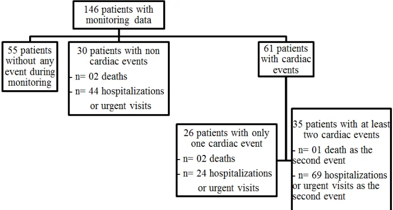
Out of the 146 monitored patients, 61 (42%) experienced a CCE during the 6-months signal acquisition. Among them, 35 (57%) experienced at least two CCE. As a whole, 96 CCE occurred
during signal acquisition: 3 deaths, 93 hospitalizations or urgent visits (Fig. 3).
3.3 Signal Score
All the SDS computed on the complete signal data are shown in Table 3.
The training set included signal data during 7 days before the first event in the 61 patients experiencing at least one CCE and before a random time-point in the remaining 85 patients who did not experience a CCE, thereby including all monitored patients. The testing set included signal data during 7 days before the second event in the 35 patients experiencing at least two CCE and before another random time
patients, thereby including 120 of the 146 monitored patients.
Comparison of SDS in the training set showed that, pressures and pulse rates were alike between patients with or without CCE. But, body weight’s slope and body weight’s standard
݈ܵ݅݃݊ܽ ݏܿݎ݁ =
+3.713 ∗ ݈ܵ݁ ሺܾ݀ݕ + 0.944 ∗ ܵܦ ሺܾ݀ݕ ݓ݁݅݃ + 0.804 ∗ ݈ܵ݁ ሺܾ݀ݕ + 0.034 ∗ ܵܦ ሺݑ݈ݏ݁ + 0.017 ∗ ܵܦ ሺݑ݈ݏ݁ − 0.020 ∗ ܯ݁ܽ݊ ሺ݀݅ܽݏݐ݈݅ܿ − 0.049 ∗ ܵܦ ሺ݂݂݀݅݁ݎ݁݊ݐ݈݅ܽ
A higher signal score was observed in a patient with an increase of body weight’s variability on 3 consecutive days, or a sustained body weight’s increase on 3 or 7 consecutive days, or an increased of pulse rate’s variability on 3 or 7 consecutive days, or a decrease in mean diastolic blood pressure on 3 consecutive days, or a narrow differential blood pressure on 3 con
body weight’s increase on 7 consecutive days was the most important feature given its highest coefficient.
Fig. 4. Impact of the L1-norm penalty The training set included signal data during 7 days before the first event in the 61 patients experiencing at least one CCE and before a point in the remaining 85 patients who did not experience a CCE, thereby including The testing set included signal data during 7 days before the second event in the 35 patients experiencing at least two CCE and before another random time-point in 85 patients, thereby including 120 of the 146
training set showed that, pressures and pulse rates were alike between patients with or without CCE. But, body weight’s slope and body weight’s standard
deviation in the 3-, 5-, and 7-days preceding the CCE were higher in patients with CCE (Table 3).
All SDS listed in Table 3 were candidate covariates introduced in the LASSO regression to build the signal score. The impact of the L norm penalty λ of the LASSO logistic regression on the coefficients of the model is shown in Fig. 4. While a complex model including the 30 initial candidate covariates was obtained when a 0 penalty was applied, most regression coefficients were sharply shrinked to 0 with increasing value of λ. With an optimal value of 3.5 for λ, the model included the seven following SDS in the signal score:
ሺܾ݀ݕ ݓ݁݅݃ℎݐ ݒ݁ݎ 7 ܿ݊ݏ݁ܿݑݐ݅ݒ݁ ݀ܽݕݏሻ ݓ݁݅݃ℎݐ ݀ݑݎ݅݊݃ 3 ܿ݊ݏ݁ܿݑݐ݅ݒ݁ ݀ܽݕݏሻ ሺܾ݀ݕ ݓ݁݅݃ℎݐ ݒ݁ݎ 3 ܿ݊ݏ݁ܿݑݐ݅ݒ݁ ݀ܽݕݏሻ
ݎܽݐ݁ ݀ݑݎ݅݊݃ 7 ܿ݊ݏ݁ܿݑݐ݅ݒ݁ ݀ܽݕݏሻ ݎܽݐ݁ ݀ݑݎ݅݊݃ 3 ܿ݊ݏ݁ܿݑݐ݅ݒ݁ ݀ܽݕݏሻ
ሺ݀݅ܽݏݐ݈݅ܿ ܾ݈݀ ݎ݁ݏݏݑݎ݁ ݀ݑݎ݅݊݃ 3 ܿ݊ݏ݁ܿݑݐ݅ݒ݁ ݀ܽݕݏሻ ݂݂݀݅݁ݎ݁݊ݐ݈݅ܽ ܾ݈݀ ݎ݁ݏݏݑݎ݁ ݀ݑݎ݅݊݃ 3 ܿ݊ݏ݁ܿݑݐ݅ݒ݁ ݀ܽݕݏሻ
A higher signal score was observed in a patient with an increase of body weight’s variability on 3 or a sustained body weight’s increase on 3 or 7 consecutive days, or an increased of pulse rate’s variability on 3 or 7 consecutive days, or a decrease in mean diastolic blood pressure on 3 consecutive days, or a narrow differential blood pressure on 3 consecutive days. A sustained body weight’s increase on 7 consecutive days was the most important feature given its highest
norm penalty λ of the LASSO logistic regression model on the coefficients
days preceding the CCE were higher in patients with CCE (Table 3).
SDS listed in Table 3 were candidate covariates introduced in the LASSO regression to build the signal score. The impact of the L1
of the LASSO logistic regression on the coefficients of the model is shown in
el including the 30 initial candidate covariates was obtained when a 0 penalty was applied, most regression coefficients were sharply shrinked to 0 with . With an optimal value of , the model included the seven following
ሻ ሻ
A higher signal score was observed in a patient with an increase of body weight’s variability on 3 or a sustained body weight’s increase on 3 or 7 consecutive days, or an increased of pulse rate’s variability on 3 or 7 consecutive days, or a decrease in mean diastolic blood pressure secutive days. A sustained body weight’s increase on 7 consecutive days was the most important feature given its highest
9
Table 3. Signal-Derived-Statistics in the 3-day, 5-day and 7-day window preceding a cardiac composite endpoint or a random time-point in patients without event, using training set
Signal derived statistics 3- day window 5- day window 7- day window
Yes No P- value Yes No P- value Yes No P- value
n =61 n = 85 n =61 n = 85 n =61 n = 85
Body weight SDa -- Kg 0.58 ± 0.46 0.41 ± 0.28 .009 0.67 ± 0.47 0.53 ± 0.32 .04 0.75 ± 0.46 0.55 ± 0.30 .002
Body weight slope – Kg/day 0.43 ± 0.29 0.29 ± 0.21 .002 0.31 ± 0.30 0.20 ± 0.18 .01 0.26 ± 0.23 0.13 ± 0.12 < .001
SBPb mean -- mmHg 123 ± 23 128 ± 22 .26 124 ± 22 127 ± 21 .32 123 ± 22 127 ± 21 .24
SBPb SDa -- mmHg 6.3 ± 4.5 6.6 ± 4.9 .65 7.1 ± 3.5 7.0 ± 4.0 .84 7.6 ± 3.8 7.1 ± 3.0 .41
DBPc mean --mmHg 74 ± 15 77 ± 15 .28 74 ± 14 76 ± 14 .38 73 ± 14 76 ± 14 .28
DBPc SDa -- mmHg 5.0 ± 3.6 5.3 ± 3.8 .60 5.9 ± 3.0 5.7 ± 3.2 .67 6.1 ± 2.8 5.8 ± 2.8 .54
BPd difference mean--mmHg 49 ± 13 51 ± 13 .48 50 ± 13 51 ± 14 .50 49 ± 12 51 ± 14 .44
BPd difference SDa -- mmHg 5.1 ± 3.4 6.0 ± 4.2 .21 6.1 ± 3.0 6.2 ± 3.4 .75 6.3 ± 2.8 6.4 ± 3.4 .87
PRe mean --ppm 79 ± 16 77 ± 14 .55 79 ± 16 77 ± 14 .50 78 ± 16 77 ± 14 .53
PRe SDa --ppm 6.4 ± 6.9 5.0 ± 4.8 .18 6.7 ± 5.9 5.4 ± 4.0 .11 6.8 ± 5.3 5.3 ± 3.7 .052
Data are mean ± SD; aSD= Standard Deviation; bSBP=Systolic Blood Pressure; cDBP=Diastolic Blood Pressure; dBP= Blood Pressure; ePR= Pulse Rate; To calculate the body
weight’s SD on a 3-days window for each patient, we computed standard deviation using the 3 consecutive values of body weight preceding the patient specific time-point. We then averaged these values by subgroups of patients with and without CCE
Table 4. Sensitivity and Specificity of BELGIUM-HF dynamic algorithms as compared with other literature’s rules, assessed in the testing set
Belgium-HF Standard “rules- of-thumb” TEMA-HF1 trial rules*
Clinical score Dynamic algorithms
MAGGIC score (cut-off = 40%)
Signal score: (cut-off = 20%)
Combined score: MAGGIC score + Signal score (cut-off = 25%)
3 lbs in 1 day
5 lbs in 3 days
Body weight ± 2kg from
discharge or SBPa outside 90-140 mmHg or PRb outside 50-90/min
Sensitivity (%) 86 60 92 5 10 79
Specificity (%) 29 78 77 96 98 31
Youden index 0.15 0.38 0.69 0.01 0.08 0.10
a
The coefficients’ paths identify the covariates to contribute to the prediction model. For the optimal value of λ (3.5), achieved by leave-one-out cross validation, the model include 7 SDS.
The signal risk score predicted CCE in the training set (AUC= 0.796), in the testing set (AUC= 0.830) and in the whole signal time-points of all patients (AUC=0.749, all P < .001, Fig. 5).
Prediction of CCE with the combined score was superior to each separate score in the training set (left panel), in the testing set (central panel), and in the whole signal (right panel).
3.4 MAGGIC Score
The MAGGIC score was predictive of CCE in the training set (AUC= 0.663), in the testing set (AUC=0.748) and in the complete set (AUC=0.649) (P < .001, Fig. 5).
3.5 Combined MAGGIC and Signal Scores
The second logistic model resulted in the following new combined score (P < .001 and P = 0.004 for statistical tests on the coefficients of signal and MAGGIC scores respectively).
ܥܾ݉݅݊݁݀ ݏܿݎ݁ =
+ 0.781
+ 1.478 ∗ ݈ܵ݅݃݊ܽ ݏܿݎ݁ + 1.031 ∗ ܯܣܩܩܫܥ ݏܿݎ݁
Prediction of CCE with the combined score was superior to each separate score in the training set (AUC=0.830), in the testing set (AUC=0.891), and when using the whole signal (AUC=0.781) with all P < .001 (Fig. 5), meaning that clinical data and signal data brought additive information to risk prediction. This is also illustrated in Fig. 6, in 5 individual patients. The MAGGIC score is a single value per patient estimated at baseline. The signal score is a daily value. Patient C with a low MAGGIC score had no event. Patients A, B, D and E with high MAGGIC score experienced each one, at least one event, all at high values of the signal score. The combined score is also a daily value. These 5 patients had similar median signal scores. But, when combining the signal score with the MAGGIC score, patients A and E with a high MAGGIC score, had a high combined score; patients B and D with a medium MAGGIC score, had a medium combined score; patient C with a low MAGGIC score, had a low combined score. This allows for an individualization of HTM.
The MAGGIC score is a single value per patient (left panel). The signal score is a daily value. A box plot represents all score values of a single patient (central and right panels). Squares indicate the score value of a patient, the day he experienced an event. Combining the MAGGIC score with the signal score induces a high increase (patients A and E), an intermediate increase (patients B and D) or a decrease (patient C) in daily values, allowing the individualization of monitoring. Cut-off can be set to trigger alerts as 25% for the combined score in this example.
3.6 Comparison of the Combined Score’s Diagnostic Accuracy with Simple Rules
Using some cut-off (40%, 20% and 25% respectively for MAGGIC, signal and combined scores), we assessed sensitivity and specificity of each of the three scores. Alarms can be set at other cut-off values, according to the targeted positive predictive value. The MAGGIC score had a high sensitivity but a low specificity whereas the signal score had a high specificity but a low sensitivity in the testing set. Combining the two scores allowed having a more effective diagnostic method with a good sensitivity (92%) and a good specificity (77%) (Table 4). Running standard “rules-of-thumb” (RoTs) showed a low sensitivity of 5% for a loss of 3 lbs in 1 day and of 10% for a loss of 5 lbs in 3 days. The rules applied in TEMA-HF1 trial [20] achieved a sensitivity of 79% but with only 31% of specificity (Table 4).
4. DISCUSSION
Fig. 5. ROC curves of the various scores for the cardiac composite endpoint (CCE)
Fig. 6. Illustration of each of the three scores in 5 individual patients
MAGGIC clinical score resulted ultimately in an efficient individualized dynamic algorithm whose predictive value was higher, whatever the cutoff, as demonstrated by ROC curves.
Combining HTM with MAGGIC score provides two main advantages. Firstly, we showed that this combination better predicted HF events than previously developed algorithms. Secondly, patients at high risk of re-hospitalization or sudden death appear to benefit more from HTM programs compared to patients with stable HF [21]. Combining HTM with MAGGIC score could well help to identify the subgroup of patients for whom this technology would be most beneficial.
Because of major differences in data collections and events definitions, indirect comparisons of our results with published algorithms are
body weight and its variability significantly improved the detection of HF events with a high sensitivity of 82% [17]. However, this sensitivity may have artificially increased because, as authors pointed out, the body weight trend itself served to comfort the diagnosis of worsening HF in 54% of patients. Our individualized dynamic algorithm also improved the detection of HF events (92% sensitivity) ensuring a valid measure of sensitivity.
There are some limitations to the present study and the small sample size is the main one. Likewise, to include negative cases in the training and testing sets, we randomly selected time-points. This could hamper the accuracy of the model specificity. Furthermore, even if signal windows used in the testing set were different from signal windows used in the training set, we cannot avoid a correlation between these two data sets because patients were the same in both sets. However, the testing set is equivalent to the training set for using the model derived in the training set. Finally, body weight gain does not occur in all patients before a HF-related event [22]. Indeed, the pathophysiology of acute decompensated HF is complex and the mechanism of this decompensation remains unclear. Whilst in some cases it is due to volume expansion, half of patients did not experience an increase in total body weight [23]. An alternative hypothesis proposed by Fallick et al. is that an autonomically mediated shift between total extracellular fluid volume and effective circulating blood volume explains the development of congestion in many patients with decompensated HF [22]. This new approach assigns sympathetic activation of the venous capacitance vessels in the setting of left ventricular dysfunction as the major driving source of elevated filling pressures [22]. Changing our thinking to incorporate strategies that target fluid shifts as well as fluid gain may bring acute and chronic benefits [23]. Remote monitoring of other clinical parameters (blood pressure, heart rate) in addition to body weight, and more, the combination with MAGGIC clinical score in our study improved the predictive value of HTM. In the future, HTM could further combine devices designed to monitor right heart hemodynamic capacity to deal with the complex pathophysiology of HF.
Nevertheless, there are several arguments proving the quality of our study. Firstly, the BELGIUM-HF dataset was made of a blind storage of automated physiological measurements and a separate inventory of
factual clinical events. This design authorized unbiased descriptions of the signal trends prior to an event’s occurrence. Secondly, by considering the monitored parameters’ characteristics that are associated with HF events, we allowed a valid measure of the sensitivity of our prediction algorithm. Thirdly, we combined the signal score with the MAGGIC score, to build an individualized dynamic algorithm whose predictive power on HF events seems more efficient.
5. CONCLUSION
In conclusion, the BELGIUM-HF study identified a new individualized dynamic algorithm which appears to be the best approach to predict HF instability that led to major factual clinical events. Combining HTM with MAGGIC score showed that signal data and clinical data provide additive information to risk prediction in HF patients. HTM technology to predict HF events should include patients’ clinical prognosis. However, further studies would be needed to confirm these findings.
COMPETING INTERESTS
Authors have declared that no competing interests exist.
REFERENCES
1. Stewart S, MacIntyre K, Hole DJ, Capewell S, McMurray JJ. More 'malignant' than cancer? Five-year survival following a first admission for heart failure. Eur J Heart Fail. 2001;3(3):315-22.
2. Cleland JG, Swedberg K, Follath F, Komajda M, Cohen-Solal A, Aguilar JC, et al. The EuroHeart Failure survey programme- A survey on the quality of care among patients with heart failure in Europe. Part 1: Patient characteristics and diagnosis. Eur Heart J. 2003;24(5):442-63. 3. Lynga P, Persson H, Hagg-Martinell A, Hagglund E, Hagerman I, Langius-Eklof A, et al. Weight monitoring in patients with severe heart failure (WISH). A randomized controlled trial. Eur J Heart Fail. 2012; 14(4):438-44.
after Transition-Heart Failure (BEAT-HF) randomized clinical trial. JAMA Intern Med. 2016;176(3):310-8.
5. Inglis SC, Clark RA, Dierckx R, Prieto-Merino D, Cleland JG. Structured telephone support or non-invasive telemonitoring for patients with heart failure. Cochrane Database Syst Rev. 2015;10:CD007228.
6. Anker SD, Koehler F, Abraham WT. Telemedicine and remote management of patients with heart failure. Lancet. 2011;378(9792):731-9.
7. Dickstein K, Cohen-Solal A, Filippatos G, McMurray JJ, Ponikowski P, Poole- Wilson PA, et al. ESC guidelines for the diagnosis and treatment of acute and chronic heart failure 2008: The Task Force for the Diagnosis and
Treatment of Acute and Chronic Heart Failure 2008 of the European Society of Cardiology. Developed in collaboration with the Heart Failure Association of the ESC (HFA) and endorsed by the European Society of Intensive Care Medicine (ESICM). Eur Heart J. 2008;29(19):2388-442.
8. Chaudhry SI, Mattera JA, Curtis JP, Spertus JA, Herrin J, Lin Z, et al. Telemonitoring in patients with heart failure. N Engl J Med. 2010;363(24): 2301-9.
9. Koehler F, Winkler S, Schieber M,
Sechtem U, Stangl K, Bohm M, et al. Impact of remote telemedical
management on mortality and
hospitalizations in ambulatory patients with chronic heart failure: The telemedical
interventional monitoring in heart failure study. Circulation. 2011;123(17):
1873-80.
10. Pandor A, Thokala P, Gomersall T,
Baalbaki H, Stevens JW, Wang J, et al. Home telemonitoring or structured
telephone support programmes after recent discharge in patients with heart failure: Systematic review and economic evaluation. Health Technol Assess. 2013; 17(32):1-207, v-vi.
11. McDonald K, Wilkinson M, Ledwidge M. Role of monitoring devices in
preventing heart failure admissions. Curr Heart Fail Rep. 2015;12(4):269-75.
12. Pocock SJ, Ariti CA, McMurray JJ,
Maggioni A, Kober L, Squire IB, et al. Predicting survival in heart failure: A
risk score based on 39 372 patients from 30 studies. Eur Heart J. 2013;34(19):1404-13.
13. Sawadogo K, Ambroise J, Vercauteren S, Castadot M, Vanhalewyn M, Col J, et al. Interaction between the Kansas City cardiomyopathy questionnaire and the
Pocock's clinical score in predicting heart failure outcomes. Qual Life Res. 2016; 25(5):1245-55.
14. Schrier RW, Abraham WT. Hormones and hemodynamics in heart failure. N Engl J Med. 1999;341(8):577-85.
15. Zhang J, Goode KM, Cuddihy PE, Cleland JG, Investigators T-H. Predicting hospitalization due to worsening heart failure using daily weight measurement: Analysis of the Trans-European Network-Home-Care Management System (TEN-HMS) study. Eur J Heart Fail. 2009;11(4): 420-7.
16. Chaudhry SI, Wang Y, Concato J, Gill TM, Krumholz HM. Patterns of weight change preceding hospitalization for heart failure. Circulation. 2007; 116(14):1549-54.
17. Ledwidge MT, O'Hanlon R, Lalor L,
Travers B, Edwards N, Kelly D, et al. Can individualized weight monitoring using
the HeartPhone algorithm improve sensitivity for clinical deterioration of heart failure? Eur J Heart Fail. 2013;15(4):447-55.
18. Pavlou M, Ambler G, Seaman SR, Guttmann O, Elliott P, King M, et al. How to develop a more accurate risk prediction model when there are few events. BMJ. 2015;351:h3868.
19. Vittinghoff E. Regression methods in biostatistics: Linear, logistic, survival, and repeated measures models. 2nd ed. New York: Springer; 2012.
20. Dendale P, De Keulenaer G,
Troisfontaines P, Weytjens C, Mullens W, Elegeert I, et al. Effect of a telemonitoring-facilitated collaboration between general practitioner and heart failure clinic on mortality and rehospitalization rates in severe heart failure: The TEMA-HF 1 (TElemonitoring in the MAnagement of Heart Failure) study. Eur J Heart Fail. 2012;14(3):333-40.
overview of systematic reviews. J Med Internet Res. 2015;17(3):e63.
22. Fallick C, Sobotka PA, Dunlap ME. Sympathetically mediated changes in capacitance: Redistribution of the venous reservoir as a cause of decompensation. Circ Heart Fail. 2011;4(5):669-75.
23. Burchell AE, Sobotka PA, Hart EC,
Nightingale AK, Dunlap ME.
Chemohypersensitivity and autonomic modulation of venous capacitance in the pathophysiology of acute decompensated heart failure. Curr Heart Fail Rep. 2013; 10(2):139-46.
_________________________________________________________________________________
© 2017 Sawadogo et al.; This is an Open Access article distributed under the terms of the Creative Commons Attribution License (http://creativecommons.org/licenses/by/4.0), which permits unrestricted use, distribution, and reproduction in any medium, provided the original work is properly cited.
Peer-review history: