On the precision of a data-driven estimate of the pseudoscalar-pole
contribu-tion to hadronic light-by-light scattering in the muon
g
−
2
Andreas Nyffeler1,a
1Institut für Kernphysik, Johann-Joachim-Becher-Weg 45, Johannes Gutenberg-Universität, D-55128 Mainz, Germany
Abstract.The evaluation of the numerically dominant pseudoscalar-pole contribution to hadronic
light-by-light scattering in the muong−2 involves the pseudoscalar-photon transition form factorFPγ∗γ∗(−Q2
1,−Q 2 2)
with P= π0, η, ηand, in general, two off-shell photons with spacelike momentaQ2
1,2. We determine which
regions of photon momenta give the main contribution for hadronic light-by-light scattering. Furthermore, we analyze how the precision of future measurements of the single- and double-virtual form factor impacts the precision of a data-driven estimate of this contribution to hadronic light-by-light scattering.
1 Introduction
The anomalous magnetic moment of the muonaμserves as an important test of the Standard Model (SM) [1]. Since several years, there is an intriguing discrepancy of 3−4σ between the experimental value [2] and the theoretical SM prediction [1, 3]. While this could be a sign of New Physics, the hadronic contributions from vacuum polar-ization (HVP) and light-by-light scattering (HLbL) have large uncertainties, which make it difficult to interpret the deviation as a clear sign of physics beyond the SM. The hadronic uncertainties need to be reduced and better con-trolled, also to fully profit from new plannedg−2 exper-iments [4]. While the HVP contribution [5] can be im-proved systematically with measurements of σ(e+e− → hadrons), the often used estimates for HLbL
aHLbL
μ = (105±26)×10−11, [6] (1)
aHLbLμ = (116±40)×10−11, [1, 7] (2)
are both based on model calculations [8–12],1which suffer from uncontrollable uncertainties, see also [15].
In this situation, a dispersive approach to HLbL was proposed recently in Refs. [16, 17], which tries to re-late the presumably numerically dominant contributions from the pseudoscalar-poles and the pion-loop to, in prin-ciple, measurable form factors and cross-sections,γ∗γ∗→
π0, η, ηandγ∗γ∗ → ππ, with on-shell intermediate pseu-doscalar states.2 The hope is that this data-driven estimate for HLbL will allow a 10% precision for these tions and that the remaining, hopefully smaller
contribu-ae-mail: nyff[email protected]
1There are attempts ongoing to calculate the HLbL contribution from
first principles in Lattice QCD. A first, still incomplete, result was ob-tained recently [13]. See also the approach proposed in [14].
2There have been objections raised at this meeting [18] about the
im-plementation of the dispersive approach for the pion-pole contribution. There should be no form factor at the external vertex [12].
tions, e.g. from axial-vectors (3π-intermediate state) and other heavier states, can be obtained within models with about 30% uncertainty to reach an overall, reliable preci-sion goal of 20% (δaHLbL
μ ≈20×10−11).
Most model evaluations ofaHLbL;μ π0(pion-pole defined in different ways [12, 16, 17] or pion-exchange with off -shell-pion form factors [1, 7]) and aHLbL;Pμ , with P =
π0, η, η, agree at the level of 15%, but the full range of estimates (central values) is much larger:
aHLbL;μ;modelsπ0 = (65±15)×10−
11 (±23%), (3)
aHLbL;Pμ;models = (87±27)×10−
11 (±31%). (4)
In this paper we study, within the dispersive ap-proach, which are the most important momentum regions for the pseudoscalar-pole contribution aHLbL;Pμ . We also analyze what is the impact of the precision of current and future measurements of the single- and double-virtual pseudoscalar transition form factor FPγ∗γ∗(−Q21,−Q22)
(TFF) [19] on the uncertainty of a data-driven estimate of this contribution to HLbL. More details can be found in Ref. [20].
2 Pseudoscalar-pole contribution
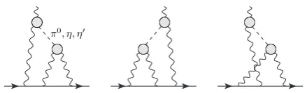
The dominant contribution to HLbL arises, according to most model calculations, from the one-particle interme-diate states of the light pseudoscalars π0, η, η shown in the Feynman diagrams in Fig. 1. We will evaluate only the pseudoscalar-pole contribution of these two-loop dia-grams. In order to simplify the notation, we mainly dis-cuss the neutral pion-pole contribution in this section. The generalization toηandηis straightforward.
The Feynman diagrams for the pion-pole contribution involve the pion TFFFπ0γ∗γ∗(q21,q22) which is defined by
00000000 00000000 00000000 00000000 00000000 00000000 00000000
11111111 11111111 11111111 11111111 11111111 11111111 11111111
0000000 0000000 0000000 0000000 0000000 0000000 0000000
1111111 1111111 1111111 1111111 1111111 1111111 1111111
π0, η, η 0000000000000000000000000000000000000000000000000
1111111 1111111 1111111 1111111 1111111 1111111 1111111
00000000 00000000 00000000 00000000 00000000 00000000 00000000
11111111 11111111 11111111 11111111 11111111 11111111 11111111
00000000 00000000 00000000 00000000 00000000 00000000 00000000
11111111 11111111 11111111 11111111 11111111 11111111 11111111
0000000 0000000 0000000 0000000 0000000 0000000 0000000
1111111 1111111 1111111 1111111 1111111 1111111 1111111
Figure 1. The pseudoscalar-pole contribution to HLbL
scat-tering. The shaded blobs represent the transition form factor
FPγ∗γ∗(q2 1,q
2
2) where P=π
0, η, η.
the QCD vertex function:
i
d4x eiq1·x0|T{jμ(x)jν(0)}|π0(q
1+q2)
=εμναβqα1q β
2Fπ0γ∗γ∗(q 2
1,q22). (5)
Here jμ(x) = (ψQˆγμψ)(x) is the light quark part of the electromagnetic current (ψ ≡ (u,d,s) and ˆQ = diag(2,−1,−1)/3 is the charge matrix). The form factor describes the interaction of an on-shell neutral pion with two off-shell photons with four-momentaq1andq2. It is Bose symmetricFπ0γ∗γ∗(q21,q22) = Fπ0γ∗γ∗(q22,q21) and for
real photons it is related to the decay widthF2
π0γ∗γ∗(0,0)=
4Γ(π0 → γγ)/(πα2m3
π). Often the normalization with the chiral anomalyFπ0γ∗γ∗(0,0)=−Nc/(12π2Fπ) is used.
The projection of the Feynman diagrams in Fig. 1 on the muong−2 leads to a two-loop integral involving the propagators of the muon, the photons, the pion, the prod-uct of two transition form factors and some kinematical functions [10]. After a Wick rotation to Euclidean menta and averaging over the direction of the muon mo-mentum, one can perform for arbitrary form factors all an-gular integrations, except one over the angle θ between the four-momentaQ1 andQ2which also appears through Q1·Q2in the form factors [1]. Writing
aHLbL;μ π0 =
α
π
3
aHLbL;μ π0(1)+aHLbL;π
0(2)
μ
, (6)
where the first contribution arises from the first two Feyn-man diagrams in Fig. 1 and the second from the last graph, one obtains the following three-dimensional integral rep-resentation for the pion-pole contribution [1]
aHLbL;μ π0(1)=
∞
0 dQ1
∞
0 dQ2
1
−1
dτ w1(Q1,Q2, τ)
× Fπ0γ∗γ∗(−Q21,−(Q1+Q2)2)Fπ0γ∗γ∗(−Q22,0), (7)
aHLbL;μ π0(2)=
∞
0 dQ1
∞
0 dQ2
1
−1d
τ w2(Q1,Q2, τ)
× Fπ0γ∗γ∗(−Q21,−Q22)Fπ0γ∗γ∗(−(Q1+Q2)2,0). (8) The integrations in Eqs. (7) and (8) run over the lengths of the two Euclidean four-momentaQ1andQ2and the angle
θbetween themQ1·Q2=Q1Q2cosθand where we intro-ducedτ=cosθ.3 From the definition of the form factor in
3We have writtenQ
i ≡ |(Qi)μ|,i = 1,2 for the length of the four vectors. Following [16] we changed the notation used in [1] and write
τ=cosθin order to avoid confusion with the Mandelstam variabletin the context of the dispersive approach.
Eq. (5) it follows that the weight functionsw1,2(Q1,Q2, τ) are dimensionless. Furthermorew2(Q1,Q2, τ) is symmet-ric underQ1 ↔ Q2 [1]. Finally,w1,2(Q1,Q2, τ) → 0 for Q1,2 → 0 and forτ → ±1. Expressions for the precise behavior ofw1,2(Q1,Q2, τ) forQ1,2 → 0 andτ → ±1, as well as forQ1,2→ ∞, can be found in Ref. [20].
The three-dimensional integral representation in Eqs. (7) and (8) separates the generic kinematics in the pion-pole contribution to HLbL, described by the model-independent weight functionsw1,2(Q1,Q2, τ), from the dependence on the single- and double-virtual TFF Fπ0γ∗γ∗(−Q2,0) andFπ0γ∗γ∗(−Q21,−Q22) in the spacelike
re-gion, which can in principle be measured, obtained from a dispersion relation (DR) [21, 22] or, as has been done so far for HLbL, modelled.
The only explicit dependence on the pseudoscalar ap-pears in the weight functionsw1,2(Q1,Q2, τ) via the mass in the pseudoscalar propagators, i.e. a factor 1/(Q2
2+m 2 P) inw1and a factor 1/((Q1+Q2)2+mP2)=1/(Q12+2Q1Q2τ+ Q2
2+m2P) inw2. Of course, also the form factors will de-pend on the type of the pseudoscalar.
3 The weight functions
w
1,2(
Q
1,
Q
2, τ
)
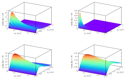
In Fig. 2 we have plotted the weight functions
w1(Q1,Q2, τ) andw2(Q1,Q2, τ) for the light pseudoscalars
π0, η, η as function of Q
1 andQ2 for θ = 90◦ (τ = 0). Three-dimensional plots for a selection of other values of θand one-dimensional plots as function ofτ = cosθ for some selected values of Q1 andQ2 can be found in Ref. [20]. Note that although the weight functions rise very quickly to the maxima in the plots in Fig. 2, the slopes along the two axis and along the diagonalQ1 =Q2 actu-ally vanish for both functions [20]. We stress that these weight functions are completely independent of any mod-els for the form factors.
We can immediately see from the weight functions for the pion that the low-momentum region,Q1,2 ≤0.5 GeV, is the most important in the corresponding integrals (7) and (8) foraHLbL;μ π0. Inw1(Q1,Q2, τ) there is a peak around Q1∼0.15−0.19 GeV,Q2∼0.09−0.16 GeV. The values of the maxima of the weight functions for all light pseu-doscalars and the locations of the maxima in the (Q1,Q2 )-plane for a selection of θ-values have been collected in Ref. [20]. Forw1(Q1,Q2, τ) andθ≤150◦, a ridge devel-ops along theQ1direction forQ2∼0.18−0.26 GeV (max-imum along the lineQ1 =2 GeV). For larger values ofθ, the function looks more and more symmetric in Q1 and Q2. This ridge leads for a constant form factor to an ultra-violet divergence (α/π)3Cln2(Λ/
mμ) for some momentum cutoff ΛwithC = 3(Nc/(12π))2(mμ/Fπ)2 = 0.0248, see
Refs. [10, 11]. Of course, realistic form factors fall offfor large momenta andaHLbL;μ π0(1)will be convergent.
0
0.5 1
1.5 2 0 0.5 1 1.5
2 0
0.51 1.52 2.53 3.54
w1
(
Q1 ,Q2
,τ
=0
)
Q1[GeV]
Q2[GeV]
w1
(
Q1 ,Q2
,τ
=0
)
0
0.5 1
1.5 2 0 0.5 1 1.5
2 0
0.05 0.1 0.15 0.2 0.25 0.3 0.35
w2
(
Q1 ,Q2
,τ
=0
)
Q1[GeV]
Q2[GeV]
w2
(
Q1 ,Q2
,τ
=0
)
0
0.5 1 1.5
2 0 0.5 1
1.5 2 0
0.1 0.2 0.3 0.4 0.5 0.6
w1
(
Q1 ,Q2
,τ
=0
)
Q1[GeV]
Q2[GeV]
w1
(
Q1 ,Q2
,τ
=0
)
0
0.5 1 1.5
2 0 0.5 1
1.5 2 0
0.05 0.1 0.15 0.2 0.25
w1
(
Q1 ,Q2
,τ
=0
)
Q1[GeV]
Q2[GeV]
w1
(
Q1 ,Q2
,τ
=0
)
Figure 2. Model-independent weight functions for theπ0: w
1(Q1,Q2, τ) (top left) andw2(Q1,Q2, τ) (top right) as function of the
Euclidean momentaQ1andQ2forθ=90◦(τ=0). Weight functionsw1(Q1,Q2, τ) forη(bottom left) andη(bottom right) forθ=90◦.
The weight functionsw2(Q1,Q2, τ) forηandηhave a similar shape as for the pion, but the peaks are broader.
of the peak moves to lower valuesQ1 =Q2 ∼0.04 GeV whenτgrows towards+1.
The dependence of the weight functions on the pseu-doscalar mass through the propagators shifts the relevant momentum regions (peaks, ridges) in the weight functions, and thus also in HLbL, to higher momenta forηcompared toπ0 and even higher forη, see Fig. 2. It also leads to a suppression in the absolute size of the weight functions due to the larger masses in the propagators. This pattern is also visible in the values for the contributions toaμ. For the bulk of the weight functions (maxima, ridges) we ob-serve the following approximate relations (not necessarily at the same values of the momenta and angles)
w1|η≈1
6 w1|π0, w1|η≈ 1
2.5 w1|η. (9)
Of course, the ratio of the weight functions is given by the ratio of the propagators and is maximal at zero momenta and at that point equal to the ratio of the squares of the masses, but at zero momenta the weight functions them-selves vanish. The combined effect is well described by the relations in Eq. (9). Furthermore, for bothηandη, the weight functionw2is about a factor 20 smaller thanw1.
The peaks for the weight functionw1(Q1,Q2, τ) forη andηare less steep, compared toπ0, and the ridge is quite broad in the Q2-direction, so that the weight function is still sizeable, compared to the maximum, forQ2=2 GeV. Furthermore, the ridge falls off only slowly in the Q1 -direction. In particular for theη, the ridge for θ ≤ 75◦
is almost as big as the maximum out to values of Q1 = 2 GeV. Forw2(Q1,Q2, τ) the peaks are broader and larger momenta contribute, compared to the pion.
For the η-meson, the peak in the weight function
w1(Q1,Q2, τ) is around Q1 ∼ 0.32−0.37 GeV, Q2 ∼ 0.22 −0.33 GeV. The peak for the weight function
w2(Q1,Q2, τ) is aroundQ1 = Q2 ∼ 0.14 GeV forτnear −1 as for the pion. The location of the peak moves down toQ1 = Q2 ∼ 0.06 GeV when τis near+1. For theη, the peak inw1(Q1,Q2, τ) now occurs for even higher mo-menta, Q1 ∼ 0.41−0.51 GeV, Q2 ∼ 0.31−0.43 GeV. The locations of the peaks ofw2(Q1,Q2, τ) in the (Q1,Q2 )-plane follow a similar pattern as for theηmeson.
4 Relevant momentum regions in
a
HLbLPμ
In order to study the impact of different momen-tum regions on the pseudoscalar-pole contribution, we need, at least for the integral with the weight function
w1(Q1,Q2, τ) in Eq. (7), some knowledge on the form factor FPγ∗γ∗(−Q21,−Q22), since the integral diverges for
a constant form factor.4 For illustration we take for the pion two simple models to perform the integrals: Low-est Meson Dominance with an additional vector multiplet, LMD+V model, based on the Minimal Hadronic Approx-imation to large-NcQCD matched to certain QCD
short-distance constraints from the operator product expansion
4The integral with the weight functionw
(OPE), see Refs. [10, 23] and references therein, and the well-known Vector Meson Dominance (VMD) model. Of course, in the end, the models have to be replaced as much as possible by experimental data on the double-virtual TFF or one can use a DR for the form factor itself [21].
The main difference of the models is a different behav-ior of the double-virtual form factor for large and equal momenta. The LMD+V model reproduces by construc-tion the OPE, whereas the VMD TFF falls offtoo fast:
FLMD+V
π0γ∗γ∗ (−Q2,−Q2)∼ FπOPE0γ∗γ∗(−Q2,−Q2)∼
1 Q2,(10) FVMD
π0γ∗γ∗(−Q2,−Q2)∼
1
Q4, for largeQ
2. (11)
Nevertheless for not too large momenta,Q1 =Q2 =Q= 0.5 [0.75] GeV, the form factorsFπ0γ∗γ∗(−Q2,−Q2) in the
two models differ by only 3% [10%], see [20]. Further-more, both models give an equally good description of the single-virtual TFFFπ0γ∗γ∗(−Q2,0) [23, 24].
The LMD+V model was developed in Ref. [23] in the chiral limit and assuming octet symmetry. This is certainly not a good approximation for the more massiveηandη mesons. For theηandηmeson we therefore simply take the usual VMD model as already done in Refs. [7, 10].
The two models yield the following results for the pole-contribution of the light pseudoscalars to HLbL (we only list here the central values)
aHLbL;μ;LMDπ+0V = 62.9×10−
11, (12)
aHLbL;μ;VMDπ0 = 57.0×10−
11, (13)
aHLbL;μ;VMDη = 14.5×10−
11, (14)
aHLbL;μ;VMDη = 12.5×10−
11. (15)
The results (12) and (13) for the pion-pole contribution in the two models are in the ballpark of many other esti-mates, but they also differ by 9.4%, relative to the LMD+V result, due to the different high-energy behavior for the double-virtual TFF in Eqs. (10) and (11) forQ1,2≥1 GeV. In fact, the pattern of the contributions toaHLbL;μ π0 is to a large extent determined by the model-independent weight functions w1,2(Q1,Q2, τ), which are concentrated below about 0.5 GeV, up to that ridge in w1 along the Q1 di-rection. As long as realistic form factor models for the double-virtual case fall offat large momenta and do not differ too much at low momenta, we expect similar results for the pion-pole contribution at the level of 15% which is in fact what is seen in the literature [1, 10, 15]. Neverthe-less, due to the ridge-like structure in the weight function
w1, the high-energy behavior of the form factors is relevant at the precision of 10% one is aiming for.
For the ηandη, the results in Eqs. (14) and (15) are as expected from the discussion of the relative size of the weight functions in Eq. (9). The result for η is about a factor 4 smaller than for the pion with VMD. The result forηis only slighly smaller than forη. Note that the nor-malization of the TFF fromΓ(P→γγ) and the momentum dependence due to different vector meson masses forηand
ηalso play a role for the results in Eqs. (14) and (15).
For a more detailed analysis, we integrate in Eqs. (7) and (8) over individual momentum bins and all anglesθ
Q1,max
Q1,min
dQ1 Q2,max
Q2,min
dQ2
1
−1
dτ (16)
and display the results, relative to the totals in Eqs. (12)-(15), in Fig. 3.
Since the absolute size of the weight function
w1(Q1,Q2, τ) is much larger thanw2(Q1,Q2, τ), the con-tribution from the integral aHLbL;μ π0(1) in Eq. (7) domi-nates overaHLbL;μ π0(2)in Eq. (8). Therefore the asymmetry seen in the (Q1,Q2)-plane in Fig. 3, with larger contribu-tions below the diagonal, reflects the ridge-like structure ofw1(Q1,Q2, τ) in Fig. 2.
For the pion, the largest contribution comes from the lowest binQ1,2 ≤0.25 GeV since a large part of the peaks in the weight functions (for different anglesθ) is contained in that bin. More than half of the contribution comes from the four bins with Q1,2 ≤0.5 GeV. In contrast, for theη andη, it is not the binQ1,2 ≤0.25 GeV which yields the largest contribution, since the maxima of the weight func-tions are shifted to higher momenta, around 0.3−0.5 GeV. Furthermore, more bins up toQ2=2 GeV now contribute at least 1% to the total. This is different from the pattern seen forπ0. The plots of the weight functions forηand
ηin Fig. 2 show that now the region 1.5−2.5 GeV also is important for the evaluation of theη- andη-pole con-tributions. The VMD model is, however, known to have a too fast fall-offat large momenta, compared to the OPE. Therefore the size of the contributionsaHLbL;μ ηandaHLbL;η
μ in Eqs. (14) and (15) might be underestimated by the VMD model, which could also affect the relative importance of the higher momentum region in Fig. 3.
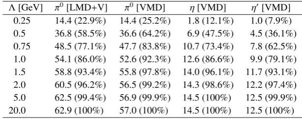
Integrating bothQ1andQ2from zero up to some up-per momentum cutoff Λand integrating over all anglesθ, one obtains the results shown in Table 1. This amounts to summing up the individual bins shown in Fig. 3.
As one can see in Table 1, for the pion more than half of the final result stems from the region belowΛ = 0.5 GeV (59% for LMD+V, 64% for VMD) and the re-gion below Λ = 1 GeV gives the bulk of the total re-sult (86% for LMD+V, 92% for VMD). The small diff er-ence between the form factor models for small momenta Q1,2 ≤ 0.5 GeV is reflected in the small absolute diff er-ence for aHLbL;μ π0 in the two models forΛ ≤ 0.75 GeV. For instance, for Λ = 0.75 GeV, the difference is only 0.8×10⁻¹¹, i.e. 1.6%. The faster fall-off of the VMD model at larger momenta beyond 1 GeV, compared to the LMD+V model, leads to a smaller contribution from that region to the total. Therefore we can see in Fig. 3 that the main contributions in the VMD model, relative to the to-tal, are concentrated at lower momenta, compared to the LMD+V model, in particular below 0.75 GeV.
Q1[GeV] Q2[GeV]
0 0.25 0.5 0.75 1.0 2.0 0
0.25 0.5 0.75 1.0 2.0
22.9% 25.2%
17.0% 18.6%
6.5% 6.8%
2.8% 2.6%
3.0% 2.0% 6.6%
7.3% 12.0% 13.1%
6.2% 6.4%
2.8% 2.6%
3.1% 2.0% 1.0%
1.0% 2.6% 2.9%
2.4% 2.4%
1.3% 1.2%
1.6% 1.0%
Q1[GeV] Q2[GeV]
0 0.25 0.5 0.75 1.0 2.0 0
0.25 0.5 0.75 1.0 2.0
12.1% 7.9%
10.0% 7.0%
3.7% 2.8%
1.4% 1.2%
1.1% 8.8%
7.1% 16.6% 14.1%
8.5% 7.8%
3.5% 3.4%
2.7% 2.9% 2.3%
2.5% 6.2% 7.0%
5.3% 6.4%
2.7% 3.5%
2.3% 3.2% 1.7%
2.5% 1.9% 2.9%
1.4% 2.2%
1.5% 2.5% 1.4%
1.0% 1.9% 1.8%
1.6% 3.3%
Figure 3.Left panel: Relative contributions to the totalaHLbL;μ π0 from individual bins in the (Q1,Q2)-plane, integrated over all angles
according to Eq. (16). Note the larger size of the bins withQ1,2 ≥1 GeV. Top line in each bin: LMD+V model, bottom line: VMD
model. Contributions smaller than 1% have not been displayed. For the LMD+V model there are further contributions bigger than
1% along theQ1-axis. For 2 GeV≤Q1 ≤20 GeV: 1.1% in the bin 0≤Q2 ≤0.25 GeV and 1.2% for 0.25 GeV≤Q2 ≤0.5 GeV.
Right panel: Relative contributions to the total ofaHLbL;μ ηandaμHLbL;ηwith the VMD model from individual bins in the (Q1,Q2)-plane,
integrated over all angles. Top line in each bin:η-meson, bottom line:η-meson.
Table 1.Pseudoscalar-pole contributionaHLbL;P
μ ×1011,P=π0, η, ηfor different form factor models obtained with a momentum
cutoff Λ. In brackets, relative contribution of the total obtained withΛ =20 GeV.
Λ[GeV] π0[LMD+V] π0[VMD] η[VMD] η[VMD] 0.25 14.4 (22.9%) 14.4 (25.2%) 1.8 (12.1%) 1.0 (7.9%) 0.5 36.8 (58.5%) 36.6 (64.2%) 6.9 (47.5%) 4.5 (36.1%) 0.75 48.5 (77.1%) 47.7 (83.8%) 10.7 (73.4%) 7.8 (62.5%) 1.0 54.1 (86.0%) 52.6 (92.3%) 12.6 (86.6%) 9.9 (79.1%) 1.5 58.8 (93.4%) 55.8 (97.8%) 14.0 (96.1%) 11.7 (93.1%) 2.0 60.5 (96.2%) 56.5 (99.2%) 14.3 (98.6%) 12.2 (97.4%) 5.0 62.5 (99.4%) 56.9 (99.9%) 14.5 (100%) 12.5 (99.9%) 20.0 62.9 (100%) 57.0 (100%) 14.5 (100%) 12.5 (100%)
5 Impact of transition form factor
uncertainties on
a
HLbL;PμFor the calculation of the pseudoscalar-pole contribution aHLbL;Pμ with P = π0, η, η in Eqs. (7) and (8) the single-virtual form factorFPγ∗γ∗(−Q2,0) and the double-virtual
form factor FPγ∗γ∗(−Q21,−Q22), both in the spacelike
re-gion, enter. We are interested here in the impact of uncer-tainties of experimental measurements of these form fac-tors on the precision ofaHLbL;Pμ . See Ref. [19] for a brief overview of the various experimental processes where in-formation on the transition form factors can be obtained. In the following, we will only quote the most relevant and most precise experimental references. Ref. [20] contains a detailed analysis of the current experimental situation.
For the single-virtual form factor FPγ∗γ∗(−Q2,0) the
following experimental information is available. The nor-malization of the form factor can be obtained from the decay width Γ(P → γγ) [25, 26]. Another important experimental information is the slope of the form fac-tor at the origin. In the spacelike region, the slope and the form factor itself have been measured in the process e+e− → e+e−γ∗γ∗ → e+e−P [27]. The extraction of the
slope requires, however, a model dependent extrapolation from rather large momentaQ∼0.5 GeV toQ2 =0. The slope and the TFF can also be obtained in the timelike re-gion from the single Dalitz-decay P→γ∗γ→+−γwith
=e, μ[28]. Of course, for the pion only the decay with an electron pair is possible. For the pion the phase space is, however, rather small and the decay is not very sensi-tive to form factor effects. The corresponding determina-tions of the slope and the TFF are rather unprecise. The situation is much better for ηandη. However, one then still needs to perform an analytical continuation to obtain the form factor at spacelike momenta. Recently a DR has been proposed in Ref. [21] to determine the single- and double-virtual form factor for the pion. So far, only the single-virtual form factor has been evaluated in this dis-persive framework with high precision at low momenta Q ≤1 GeV. For theηandη, a dispersive approach for the single- and double-virtual TFF has been presented in Ref. [22].
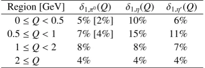
For the single-virtual form factor we parametrize the measurement errors in Eqs. (7) and (8) as follows:
The momentum dependent errorsδ1,P(Q) in different bins are displayed in Table 2, based on the analysis in Ref. [20]. There are currently no experimental data for the form factor available in the spacelike region in the lowest bin 0 ≤ Q<0.5 GeV forπ0andη, except fromΓ(P → γγ), the slope and timelike data for theη-TFF. For the lowest bin we therefore assume an error, based on “extrapolating” the current data sets and the data that will be available soon from BES III [29] and maybe from KLOE-2 [24] for the pion. If one uses the DR from Ref. [21] below 1 GeV [30] and the current error on the normalization from the decay width, one obtains (conservatively) the uncertainties in the lowest two bins given in brackets in Table 2.
Table 2.Relative errorδ1,P(Q) on the form factorFPγ∗γ∗(−Q2,0)
for P=π0, η, ηin different momentum regions. The errors for
δ1,π0(Q) andδ1,η(Q) below 0.5 GeV are based on assumptions.
In brackets forπ0the uncertainties with a DR for the TFF.
Region [GeV] δ1,π0(Q) δ1,η(Q) δ1,η(Q)
0≤Q<0.5 5% [2%] 10% 6% 0.5≤Q<1 7% [4%] 15% 11%
1≤Q<2 8% 8% 7%
2≤Q 4% 4% 4%
The second ingredient in Eqs. (7) and (8) is the double-virtual form factorFPγ∗γ∗(−Q2
1,−Q 2
2). Currently, there are no direct experimental measurements available for this form factor at spacelike momenta. For the pion, from the double Dalitz decayπ0 →γ∗γ∗→e+e−e+e−, one can ob-tain the double-virtual form factor|Fπ0γ∗γ∗(q21,q22)|at small
invariant momenta in the timelike region, but the results are inconclusive [31]. There is indirect information avail-able on the double-virtual TFF from the loop-induced de-cay P → +− ( = e, μ) [25, 32]. Without a form fac-tor at the P−γ∗−γ∗-vertex, the loop integral is ultravi-olet divergent. The relation between this decay and the pseudoscalar-pole contribution aHLbL;Pμ has been stressed in Ref. [11] and problems to explain both processes simul-taneously with the same model have been pointed out [33]. In this situation, models have been used to describe the form factorFPγ∗γ∗(−Q2
1,−Q 2
2) in the spacelike region and thus all current evaluations of aHLbL;Pμ are model depen-dent. Of course, it would be preferable to replace these model assumptions as much as possible by experimental data. In fact, it is planned to determine the double-virtual form factor, at least for the pion, at BES III for momenta 0.5 ≤ Q1,2 ≤ 1.5 GeV and a first analysis is already in progress [29], based on existing data.
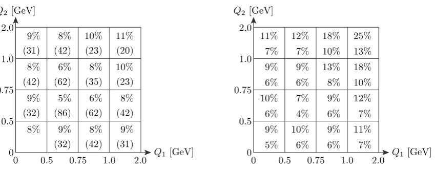
In analogy to the single-virtual form factor, we parametrize potential future measurement errors for the double-virtual form factor in Eqs. (7) and (8) in the fol-lowing, simplifying way:
FPγ∗γ∗(−Q21,−Q22)
→ FPγ∗γ∗(−Q21,−Q22)1±δ2,P(Q1,Q2), (18)
where the assumed momentum dependent errors
δ2,P(Q1,Q2) in different bins are shown in Fig. 4. The error estimate for the form factor in each bin has been
obtained based on a Monte Carlo (MC) simulation [29] for the BES III detector using the LMD+V model in the EKHARA event generator [34] for the signal process e+e−→ e+e−γ∗γ∗ →e+e−π0and the VMD model for the production ofηandη. Since the number of eventsNiin
bin number i is proportional to the cross-section σi (in that bin) and since for the calculation of the cross-section the form factor enters squared, the statistical error on the form factor measurement is given according to Poisson statistics byσi∼ FP2γ∗γ∗⇒δFPγ∗γ∗/FPγ∗γ∗= √Ni/(2Ni).
In the lowest momentum binQ1,2≤0.5 GeV, there are no events in the simulation, because of the acceptance of the detector. When bothQ2
1,2are small, both photons are almost real and the scattered electrons and positrons es-cape detection along the beam pipe. As a further assump-tion, we have therefore taken the average of the uncertain-ties in the three neighboring bins as estimate for the error in that lowest bin. This “extrapolation” from the neighbor-ing bins seems justified, since information along the two axis is (or will soon be) available and the value at the origin is known quite precisely from the decay width. Note that although the form factor for spacelike momenta is rather smooth, it is far from being a constant and some nontrivial extrapolation is needed. For instance, for the pion we get Fπ0γ∗γ∗(−(0.5 GeV)2,−(0.5 GeV)2)/Fπ0γ∗γ∗(0,0)≈0.5, for
both the LMD+V and the VMD model [20].
The MC simulation [29] corresponds to a data sample of approximately half of the data collected at BES III so far. The simulation included only signal events. Based on a first preliminary analysis of the BES III data [29] with strong cuts to reduce the background from Bhabha events with additional photons, it seems possible, at least for the pion, that the number of events and the correspond-ing precision forFπ0γ∗γ∗(−Q21,−Q22) shown in Fig. 4 could
be achievable with the current data set plus a few more years of data taking. Of course, once experimental data will be available, e.g. event rates in the different momen-tum bins, there will still be the task to unfold the data to reconstruct the form factor FPγ∗γ∗(−Q2
1,−Q 2
2) without in-troducing too much model dependence.
Taking the LMD+V and VMD models for illustration, the assumed momentum dependent errors from Table 2 and Fig. 4 impact the precision for the pseudoscalar-pole contributions to HLbL as follows
aHLbL;μ;LMDπ+0V = 62.9+ 8.9 −8.2×10−
11 +14.1% −13.1%
, (19)
aHLbL;μ;VMDπ0 = 57.0+ 7.8
−7.3×10⁻¹¹ +13 .7% −12.7%
, (20)
aHLbL;μ;VMDη = 14.5+ 3.4
−3.0×10⁻¹¹ +23 .4% −20.8%
, (21)
aHLbL;μ;VMDη = 12.5+ 1.9
−1.7×10⁻¹¹ +15 .1% −13.9%
. (22)
Q1[GeV]
Q2[GeV]
0 0.5 0.75 1.0 2.0
0 0.5 0.75 1.0 2.0
8% 9%
(32) 8% (42)
9% (31) 9%
(32) 5% (86)
6% (62)
8% (42) 8%
(42) 6% (62)
8% (35)
10% (23) 9%
(31) 8% (42)
10% (23)
11% (20)
Q1[GeV]
Q2[GeV]
0 0.5 0.75 1.0 2.0
0 0.5 0.75 1.0 2.0
9% 5%
10% 6%
9% 6%
11% 7% 10%
6% 7% 4%
9% 6%
12% 7% 9%
6% 9% 6%
13% 8%
18% 10% 11%
7% 12%
7% 18% 10%
25% 13%
Figure 4.Left panel: Assumed relative errorδ2,π0(Q1,Q2) on the pion TFFFπ0γ∗γ∗(−Q21,−Q22) in different momentum bins. Note the
unequal bin sizes. In brackets the number of MC eventsNiin each bin according to the simulation with the LMD+V model for BES
III. For the lowest bin,Q1,2 ≤0.5 GeV, there are no events in the simulation due to the detector acceptance. In that bin, we assume
as error the average of the three neighboring bins. ForQ1,2≥2 GeV, we take a constant error of 15%. Right panel: Assumed relative
errorδ2,P(Q1,Q2) on the form factorFPγ∗γ∗(−Q2
1,−Q 2
2) forP=η, ηin different momentum bins according to the MC simulations with
the VMD form factor forη(top line) andη(bottom line). ForQ1,2≥2 GeV, we assume a constant error of 25% forηand 15% forη.
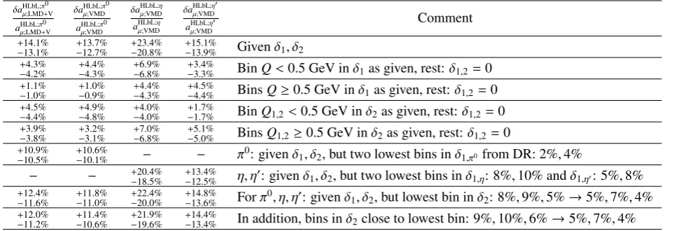
More details have been collected in Table 3, which contains the results for the relative uncertainties from Eqs. (19)-(22) in the first line. For the pion, the largest uncertainty of about 5% comes from the lowest binQ1,2≤ 0.5 GeV in the (Q1,Q2)-plane forδ2in Fig. 4 (fourth line in the table). Some improvement could be achieved, if the error in that lowest bin and the neighboring bins could be reduced, to a total error of about 12%, see the lines 8 and 9 in Table 3. The second largest uncertainty of 4.4% for the pion stems from the lowest bin Q < 0.5 GeV in δ1 (second line in the table). Here the use of a dispersion re-lation for the single-virtual form factorFπ0γ∗γ∗(−Q2,0) for
Q<1 GeV (see values in brackets in Table 2) could bring the total error of 14% down to 11%, see the sixth line.
For theηmeson, the largest uncertainties of 7% orig-inate from the region ofδ2 above 0.5 GeV (5th line) and from the lowest bin inδ1(2nd line). For theη, the largest uncertainty of 5% comes again from the region ofδ2above 0.5 GeV (5th line). The second largest uncertainty of 4.5% comes from bins inδ1above 0.5 GeV (3rd line). Forηand
ηthe errors go down to 20% and 13%, if the uncertainty in the two lowest bins inδ1 could be reduced, see line 7 in Table 3. There is only a small reduction of the uncer-tainty by one percentage point, if the errors in the lowest few bins ofδ2could be reduced further, see lines 8 and 9.
6 Conclusions
The three-dimensional integral representation for the pseudoscalar-pole contributionaHLbL;Pμ with P=π0, η, η, from Ref. [1] allows one to separate the generic kine-matics, described by model-independent weight functions
w1,2(Q1,Q2, τ), from the double-virtual transition form factorsFPγ∗γ∗(−Q21,−Q22). From the weight functions one
deduces that the relevant momentum regions are below 1 GeV forπ0and below about 1.5 GeV forηandη.
If the assumed measurement errors δ1(Q) and
δ2(Q1,Q2) on the single- and double-virtual TFF can be achieved in the coming years (in particular by measure-ments of the double-virtual form factors at BES III), one could obtain the following, largely data driven, uncertain-ties for the pseudoscalar-pole contributions to HLbL:
δaHLbL;π0
μ /aHLbL;π
0
μ = 14% [11%], (23)
δaHLbL;μ η/aHLbL;μ η = 23%, (24)
δaHLbL;η μ /aHLbL;η
μ = 15%. (25)
The result in bracket for the pion uses the DR [21] for the single-virtual TFFFπ0γ∗γ∗(−Q2,0). Compared to the range
of estimates in the literature given in Eqs. (3) and (4) this would definitely be some progress. More work is needed, however, to reach a precision of 10% for all three contri-butions. Experimental data on the double-virtual form fac-tors in the region 0−1.5 GeV, e.g. from KLOE-2 or Belle 2, would be very helpful in this respect. A more detailed discussion can be found in [20].
Acknowledgements
Table 3.Impact of assumed measurement errorsδ1,P(Q) andδ2,P(Q1,Q2) in the form factorsFPγ∗γ∗(−Q2,0) andF Pγ∗γ∗(−Q2
1,−Q 2 2) on
the relative precision of the pseudoscalar-pole contributions (first line). Lines 2−5 show the effects of uncertainties in different
momentum regions below and above 0.5 GeV. Lines 6−9 show the impact of potential improvements of some of the assumed errors.
δaHLbL;μ;LMDπ+0V
aHLbL;π0
μ;LMD+V
δaHLbL;μ;VMDπ0
aHLbL;π0
μ;VMD
δaHLbL;μ;VMDη
aHLbL;μ;VMDη
δaHLbL;μ;VMDη
aHLbL;η
μ;VMD
Comment
+14.1%
−13.1% +13
.7%
−12.7% +23
.4%
−20.8% +15
.1%
−13.9% Givenδ1, δ2 +4.3%
−4.2% +4
.4%
−4.3% +6
.9%
−6.8% +3
.4%
−3.3% BinQ<0.5 GeV inδ1as given, rest:δ1,2=0 +1.1%
−1.0% +1
.0%
−0.9% +4
.4%
−4.3% +4
.5%
−4.4% BinsQ≥0.5 GeV inδ1as given, rest:δ1,2 =0 +4.5%
−4.4% +4
.9%
−4.8% +4
.0%
−4.0% +1
.7%
−1.7% BinQ1,2<0.5 GeV inδ2as given, rest:δ1,2 =0 +3.9%
−3.8% +3
.2%
−3.1% +7
.0%
−6.8% +5
.1%
−5.0% BinsQ1,2≥0.5 GeV inδ2as given, rest:δ1,2=0 +10.9%
−10.5% +10
.6%
−10.1% − − π0: givenδ1, δ2, but two lowest bins inδ1,π0from DR: 2%,4%
− − +20.4%
−18.5% +13
.4%
−12.5% η, η: givenδ1, δ2, but two lowest bins inδ1,η: 8%,10% andδ1,η: 5%,8% +12.4%
−11.6% +11
.8%
−11.0% +22
.4%
−20.0% +14
.8%
−13.6% Forπ0, η, η: givenδ1, δ2, but lowest bin inδ2: 8%,9%,5%→5%,7%,4% +12.0%
−11.2% +11
.4%
−10.6% +21
.9%
−19.6% +14
.4%
−13.4% In addition, bins inδ2close to lowest bin: 9%,10%,6%→5%,7%,4%
References
[1] F. Jegerlehner and A. Nyffeler, Phys. Rept. 477, 1 (2009).
[2] G. W. Bennettet al., Phys. Rev. D73, 072003 (2006). [3] T. Blumet al., arXiv:1311.2198; talks at this
meet-ing: M. Knecht; K. Melnikov. [4] D. Hertzog, talk at this meeting.
[5] Talks on HVP at this meeting: M. Benayoun, arXiv:1511.01329; S. Eidelman; F. Jegerlehner, arXiv:1511.04473; M. Petschlies; M. Steinhauser; L. Trentadue; Z. Zhang, arXiv:1511.05405.
[6] J. Prades, E. de Rafael and A. Vainshtein, Adv. Ser. Direct. High Energy Phys. 20, 303 (2009) [arXiv:0901.0306].
[7] A. Nyffeler, Phys. Rev. D79, 073012 (2009). [8] M. Hayakawa, T. Kinoshita and A. I. Sanda, Phys.
Rev. Lett.75, 790 (1995); M. Hayakawa and T. Ki-noshita, Phys. Rev. D57, 465 (1998) [66, 019902(E) (2002)].
[9] J. Bijnens, E. Pallante and J. Prades, Phys. Rev. Lett.
75, 1447 (1995) [75, 3781(E) (1995)]; Nucl. Phys. B
474, 379 (1996); Nucl. Phys. B626, 410 (2002). [10] M. Knecht and A. Nyffeler, Phys. Rev. D65, 073034
(2002).
[11] M. Knechtet al., Phys. Rev. Lett.88, 071802 (2002). [12] K. Melnikov and A. Vainshtein, Phys. Rev. D 70,
113006 (2004).
[13] T. Blumet al., Phys. Rev. Lett.114, 012001 (2015); T. Blumet al., arXiv:1510.07100.
[14] J. Green et al., arXiv:1507.01577; J. Green et al., arXiv:1510.08384.
[15] Talks on HLbL at this meeting: J. Bijnens, arXiv:1510.05796; L. Cappiello; D. Greynat; C. Lehner; P. Masjuan; M. Procura.
[16] G. Colangelo et al., JHEP 1409, 091 (2014); G. Colangelo et al., Phys. Lett. B 738, 6 (2014); G. Colangeloet al., JHEP1509, 074 (2015). [17] V. Pauk and M. Vanderhaeghen, arXiv:1403.7503;
Phys. Rev. D90, 113012 (2014).
[18] A. Vainshtein, talk at this meeting.
[19] E. Czerwinski et al., arXiv:1207.6556; talks at this meeting: A. Kupsc; P. Masjuan.
[20] A. Nyffeler, work in preparation.
[21] M. Hoferichteret al., Eur. Phys. J. C74, 3180 (2014). [22] C. Hanhartet al., Eur. Phys. J. C73, 2668 (2013) [75, 242(E) (2015)]; C. W. Xiaoet al., arXiv:1509.02194. [23] M. Knecht and A. Nyffeler, Eur. Phys. J. C21, 659
(2001).
[24] D. Babusciet al., Eur. Phys. J. C72, 1917 (2012); D. Moricciani, talk at this meeting.
[25] K. A. Oliveet al.[Particle Data Group], Chin. Phys. C38, 090001 (2014).
[26] I. Larinet al., Phys. Rev. Lett.106, 162303 (2011); D. Babusciet al., JHEP1301, 119 (2013).
[27] H. Aihara et al., Phys. Rev. Lett. 64, 172 (1990); H. J. Behrend et al., Z. Phys. C 49, 401 (1991); J. Gronberg et al., Phys. Rev. D 57, 33 (1998); M. Acciarri et al., Phys. Lett. B 418, 399 (1998); B. Aubertet al., Phys. Rev. D 80, 052002 (2009); P. del Amo Sanchezet al., Phys. Rev. D84, 052001 (2011); S. Ueharaet al., Phys. Rev. D86, 092007 (2012).
[28] R. Arnaldi et al., Phys. Lett. B 677, 260 (2009); P. Aguar-Bartolomeet al., Phys. Rev. C89, 044608 (2014); M. Ablikimet al., Phys. Rev. D92, 012001 (2015).
[29] A. Denig, C. Redmer and P. Wasser, private comm. [30] M. Hoferichter and B. Kubis, private comm. [31] E. Abouzaid et al., Phys. Rev. Lett. 100, 182001
(2008).
[32] E. Abouzaidet al., Phys. Rev. D75, 012004 (2007). [33] M. J. Ramsey-Musolf and M. B. Wise, Phys. Rev. Lett. 89, 041601 (2002); A. E. Dorokhov and M. A. Ivanov, JETP Lett.87, 531 (2008); P. Masjuan and P. Sanchez-Puertas, arXiv:1504.07001.
[34] H. Czy˙z and S. Ivashyn, Comput. Phys. Commun.