Extensions of the Cross-Entropy Method with Applications to Diffusion Processes and Portfolio Losses

(1)

Scholarship@Western

Electronic Thesis and Dissertation Repository

4-16-2015 12:00 AM

Extensions of the Cross-Entropy Method with Applications to

Diffusion Processes and Portfolio Losses

Alexandre Scott

The University of Western Ontario

Supervisor Adam Metzler

The University of Western Ontario

Graduate Program in Applied Mathematics

A thesis submitted in partial fulfillment of the requirements for the degree in Doctor of Philosophy

Follow this and additional works at: https://ir.lib.uwo.ca/etd

Part of the Other Applied Mathematics Commons, and the Probability Commons

Recommended Citation Recommended Citation

Scott, Alexandre, "Extensions of the Cross-Entropy Method with Applications to Diffusion Processes and Portfolio Losses" (2015). Electronic Thesis and Dissertation Repository. 2858.

https://ir.lib.uwo.ca/etd/2858

This Dissertation/Thesis is brought to you for free and open access by Scholarship@Western. It has been accepted for inclusion in Electronic Thesis and Dissertation Repository by an authorized administrator of

(2)

Applications to Diffusion Processes and

Portfolio Losses

(Thesis Format: Integrated-Article)

by

Alexandre Scott

Graduate Program in Applied Mathematics

A thesis submitted in partial fulfillment

of the requirements for the degree of

Doctor of Philosophy

The School of Graduate and Postdoctoral Studies

Western University

London, Ontario, Canada

c

(3)

Rare event simulation is a crucial part of simulations. In financial mathematics, the study of rare events appear naturally when we consider risk measures such as the conditional value at risk. This thesis is composed of three related papers treating the rare event simulations subject: the first paper addresses rare event simulations for diffusion processes, the second paper addresses rare event simulations for the normal and the Studentt-copula model while the last paper addresses rare event simulations for a portfolio model where there is a correlation structure between the loss-given-default and the probability of loss-given-default.

Keywords: cross-entropy, Kullback-Leibler divergence, rare event simulations, loss estimation, Radon-Nykodym derivative, Importance Sampling.

(4)

My papers have all been written with Adam Metzler. I, Alexandre Scott, am the principal author.

(5)

I would like to thank the staff at the University of Western Ontario for their support. I would like to thank Adam Metzler, Mark Reesor, Matt Davison and Greg Reid for their advices and help when needed. I would also like to thank my parents, Marc and Sylvie and my brothers Maxime and Dominick who have always been very supportive. Finally, I would like to thank NSERC and FQRNT for their financial support.

(6)

List of Tables

Table 3.1 This table compares the performance of the proposed algorithm to the performance of the Glasserman and Li (2005) algorithm. We assume there are ten groups and fifteen risk factors. Factor loadings, marginal default probabilities and relative exposures can be found in Appendix C. Note that factor loadings are cho-sen to ensure that |ag|2 ≤ 0.11, meaning a low correlation

envi-ronment. In all cases obligors are divided equally across groups. i.e. Ng =N/G. . . 57

Table 3.2 This table compares the performance of the proposed algorithm to the performance of the algorithm proposed by Chan and Kroese (2010). Base parameters are N = 2000, ν = 15, ai = 0.3 and

P Di = 0.029 for alli, x= 0.4. CPU Time is given in seconds. . 63

Table 3.3 This table compares the performance of the IS estimator (3.17) to that of the crude estimator, when estimating the conditional tail expectation _E[LN|LN ≥ x] in the t copula model. Portfolio

consists of N = 500 obligors, evenly distributed among G = 10 groups (i.e. Ng = 50 for eachg), and there are D= 15 Gaussian

risk factors. Degrees of freedom are ν = 5. Default probabilities, factor loadings and exposures are given in Appendix C, and loss given defaults are all set to 100%. For each value of x in the table, 20 realizations of each estimator were simulated usingM = 10,000 in each case. Reported mean and standard deviation are the sample mean and sample standard deviation of the 20 realizations. A reported value of NA means that at least one of the 20 samples of 10,000 did not contain a single observation for which LN ≥ x, in which case both numerator and denominator

of the crude estimator is zero. The reported value of _P(LN ≥x)

is based on an IS estimate using a sample of size 200,000. . . . 64 Table 4.1 Performance of the first-stage estimator and the two-stage

esti-mator when P D = 0.029, a = 0.63, b = 0.975, ρ = 0.2, x = 0.1, β = 0.25, RLGD =

√

0.0588, RP D = 0.25 and 200 obligors.

We used 1,000,000 simulations for each estimator. . . 81

(9)

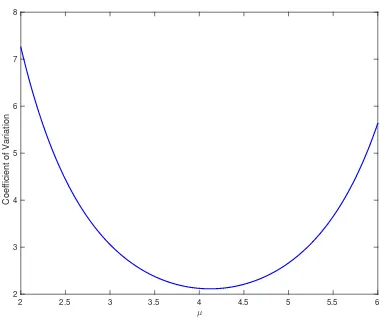
Figure 1.1 Coefficient of variation for estimating P(W1 >4) against µ. . . 6

Figure 2.1 Average path against time . . . 21 Figure 2.2 Comparison between ˆα and α_e . . . 24 Figure 2.3 Quadratic fit for v(α) . . . 24 Figure 2.4 Estimated coefficient of variation against the probability . . . . 30 Figure 2.5 Estimated coefficient of variation against the probability

estimat-ing a non-trivial function . . . 31 Figure 2.6 Estimated coefficient of variation versus the estimated

probabil-ity for the First-Stage estimator, Two-Stage estimator with con-stant drift and the Two-Stage estimator with piecewise concon-stant drift. . . 33 Figure 3.1 100 simulated pairs (LN,E[LN|Z]) in the single-factor (i.e. d =

1) homogeneous Gaussian copula model. Parameters are N = 1000, P Di = P D = 0.02, and ai = 0.2 for all i. The empirical

correlation between the two series exceeds 90%. . . 52 Figure 3.2 Average absolute error betweenEe[L_N|Z =z] and max{E[L_N|Z =

z], x} in the single-factor (i.e. d = 1) Gaussian copula model. Parameters areN = 200, P Di = 0.02, ai = 0.2 for alli. For each

value of x, we simulated 10,000 values of Z and for each value of Z we computed Ee[LN|Z = z] using the fact that N ·LN|Z =

z ∼ Bin(N, p(z)). The error Ee[L_N|Z]−max(x, `_N(z)) was then

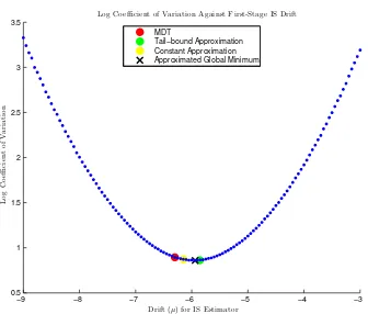
averaged across all simulated values and the solid blue line is a cubic spline fitted to that averaged data. The maximum error is located near x = P D (point in red), and we recall that in the rare event setting one is typically interested in xP D. . . 55 Figure 3.3 This figure illustrates the near-optimal performance of the

pro-posed algorithm in the single-factor homogeneous Gaussian model. The horizontal axis is the tilt parameter used in the first stage (in all cases (3.14) is used in the second stage) and the vertical axis is the log of the estimated coefficient of variation (estimated using 1,000,000 simulations). Other parameters are N = 1000,

x= 0.2,ai = 0.2,P Di = 0.02 for all i. . . 56

(10)

posed algorithm in the two-factor inhomogeneous Gaussian model. Contour plot ofCV(µ) whereCV(µ) is the coefficient of variation assuming the first stage tilt parameter is µ∈_R2 _{and the second}

stage tilt parameter is ˆθ•. CV(µ) is estimated by Monte Carlo

using 1,000,000 simulations. Parameters are a1 = [0.1 0.1]T,

a2 = [0.1 0.2]T, P D = [0.025 0.0145]T, x= 0.2 with 500 assets

distributed equally among each group (i.e. N1 =N2 = 250). . . 57

Figure 3.5 100 simulated pairs (LN,E[LN|Z]) in thetcopula model.

Param-eters are N = 1000, ν = 15, P Di =P D = 0.02 and ai = 0.3 for

all i. The empirical correlation between the two series exceeds 98%. . . 59 Figure 4.1 Order of magnitude of the estimated probability _P(LN > x)

against the threshold. The parameters area= 0.63, b= 0.975, P D = 0.029, RLGD =

√

0.0588, RP D = 0.25, ρ = 0.2, β = 0.25 with

200 obligors. We used 1,000,000 simulations per point. . . 83 Figure 4.2 Coefficient of variation of the estimator for _P(LN > x) against

the threshold. The parameters are a = 0.63, b = 0.975, P D = 0.029, RLGD =

√

0.0588, RP D = 0.25, ρ = 0.2, β = 0.25 with

200 obligors. We used 1,000,000 simulations per point. . . 84 Figure 4.3 Average iterations required for two-stage entropy algorithm against

the threshold. The parameters are a = 0.63, b = 0.975, P D = 0.029, RLGD =

√

0.0588, RP D = 0.25, ρ = 0.2, β = 0.25 with

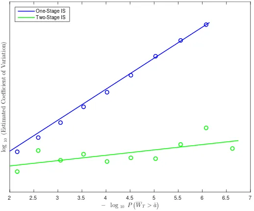
200 obligors. We used 1,000,000 simulations per point. . . 85 Figure 4.4 Order of magnitude of the coefficient of variation of the

estima-tion of_P(LN|LN > x) for the One-Stage entropy criteria and the

two-stage entropy criteria. The parameters are a = 0.63, b = 0.975, P D = 0.029, RLGD =

√

0.0588, RP D = 0.25, ρ =

0.2, β = 0.25 with 200 obligors. We used 100,000 simulations per point. . . 86

(11)

A Supplementary Results and Proofs 91

B Useful Conditional Expectations for Standard Brownian Motion 96

B.1 Large Maximum . . . 96 B.2 Large Maximum and Small Minimum . . . 97

C Parameters 100

D Equations 102

E Algorithms 104

Bibliography 113

(12)

List of Abbreviations, Symbols,

Nomenclature

Cφ(W, N) Poisson kernel estimator

F Lamperti Transform

`N(Z) Asymptotic approximation ofLN given Z

LN Loss on a portfolio of N obligors

P Di Marginal default probability for obligor i

Ψ(λ) Cumulant generating function

ψr(θ) Cumulant generating function conditioned on R=r

e

P Conditional measure of P

Wt Standard Brownian Motion

Wθ Brownian Motion with deterministic drift θt

X Running maximum of the stochastic process X X Running minimum of the stochastic process X

(13)

Chapter 1 Introduction

Monte Carlo simulation is an incredibly powerful and versatile computational method for stochastic models. A crude Monte Carlo estimator can easily and rapidly be applied to a variety of problems, however there are many cases where the crude Monte Carlo estimator fails to provide satisfactory estimates. For example, let us suppose that a bank has set aside five million capital reserves against losses on a corporate portfolio. The bank needs to estimate (i) the probability that losses exceed this reserve level and (ii) the expected shortfall (i.e. expected loss given that losses exceed 5 million). If the true probability is 0.1%, then only 1 simulation out of 1,000 is informative for (ii) and this is very problematic since computational budgets are limited in practice.

To accelerate the rate at which informative scenarios are generated, one can use Importance Sampling in conjunction with Monte Carlo simulations. In this thesis, we consider problems of the form

Ef(X)·1{X∈A}

, (1.1)

(14)

E[f(X)|X∈A] = E

f(X)·1{X∈A}

E1{X∈A}

.

Let

1{X∈A} =

1 if X ∈A

0 otherwise.

and wheref is a real-valued function,Xis a random element mapping to an arbitrary space G and A is a subset ofG. In practice, it is often impossible to compute (1.1) directly, thus Monte Carlo is the only feasible option. A naive scheme can easily be implemented as follows

1. Generate N independent copies of the random element X. We shall refer to

X(i) as theith simulated copy. 2. Return

1

N

X

i=1

f(X(i))·Yi,

where Yi =1{X(i)_∈_A_}.

We are interested in the behaviour off(X) overAbut if_P(X ∈A) is small then very few simulated values are informative. This manifests itself in an unacceptably large coefficient of variation (CV), defined as the ratio of an estimator’s standard deviation to its expected value. The standard error can be controlled by using a very large number of simulations, but in practice, this can be prohibitively expensive.

(15)

then need to implement an acceptance rejection algorithm, but when if the tilted dis-tribution does not bear enough resemblance to the original disdis-tribution, we might end up with a very low acceptance probability as discussed in Chapter 4. For control variates, it is not exactly clear how to compute the needed parameters outside of the homogeneous model without having to resort to using pre-simulations to approximate our optimal parameters. In this thesis, we propose Importance Sampling estimators to improve the performance of the estimators for two reasons: firstly, we are able to exploit Girsanov in Chapter 2 and bring back our problem to simulating Brownian Motions with deterministic drifts and secondly, we are able to use the asymptotic behaviour of large portfolios in Chapter 3 and Chapter 4 to rapidly compute the parameters for our IS estimators.

Recall that, using IS estimators, (1.1) can be rewritten as

Ef(X)·1{X∈A}

=_EQ

f(X)·1{X∈A} ·

d_P d_Q

, (1.2)

where _EQ_{[·] denotes the expected value under measure}

Q, ddQP denotes the

Radon-Nykodym derivative (RND) and where _P is a measure dominated by _Q (if _Q(x ∈

(16)

Example 1.0.1. Let Wt be a standard Brownian Motion and consider the problem

of estimating

P(W1 > a),

where a >0. By the properties of the Brownian Motion, we know that _P(W1 > a) =

Φ(−a), where Φ(·) denotes the cdf of a standard normal distribution. If a = 4, then

P(W1 > a)≈3.17×10−5. Using the naive estimator and 1,000,000 simulations, we

obtain the following estimate for _P(W1 > a):

ˆ

p= 2.70×10−5, ˆσ= 5.20×10−3,

which leads to an approximate CV of 192.60. Let us consider an IS measure, _Qµ_,

where Wt is a Brownian Motion with drift µ, i.e Qµ(Wt∈dz) = φ(z, µ,

√

t)dz, where

φ(·, µ,√t) denotes a normal pdf with mean µ and variance t. Intuitively, choosing

large positive µ should steer more trajectories upwards, and this should make the

simulations more informative. Using the right-hand side of (1.2) as the IS estimator

with µ=a, we obtain

e

p= 3.16×10−5, _eσ= 6.72×10−5,

which leads to a coefficient of variation of2.13. The above estimation is very accurate,

and one could suspect that increasingµwould only result in a better estimator. Using

the same IS estimator when µ= 8, we obtain

e e

p= 3.08×10−5, e e

σ= 3.30×10−3.

This leads to a coefficient of variation of 107.14, which is almost as inaccurate as

(17)

RND is becoming increasingly large, and the trade-off between the two can be measured

by looking at the coefficient of variation c(a, µ) defined as

c(a, µ) =

r

VarQµh₁

{WT>a}·

dP

dQµ

i

EQµ

h

1{WT>a}·

dP

dQµ

i =

s

eµ2

Φ(−a−µ)

Φ(−a)2 −1. (1.3)

Minimizing (1.3) with respect to µ (assuming a fixed) is equivalent to solving the

non-linear equation below

2µ= φ(−a−µ)

Φ(−a−µ). (1.4)

If we assume that µ increases as a increases, then as a+µ→ ∞, the right-hand side

of (1.4) is asymptotically equivalent to

φ(−a−µ)

Φ(−a−µ) ∼a+µ.

Therefore, it follows that (1.4) is asymptotically equivalent to

µ∼a,

which explains why our first estimator performs so well. Therefore, the optimal

trade-off (for this example) between IS measures too similar and not similar enough is to

have about 50% of the simulations to lie in the region where {W1 > a}.

(18)

µ

2 2.5 3 3.5 4 4.5 5 5.5 6

Coefficient of Variation

2 3 4 5 6 7 8

Figure 1.1: Coefficient of variation for estimating P(W1>4) againstµ.

1.1 The Cross-Entropy Method

The cross-entropy methodology is a well-established method to determine how sim-ilar two measures are (see Asmussen and Glynn (2007) and references therein for a comprehensive treatment of the methodology). It has been introduced by Rubinstein (1997) and although it has been applied to a wide variety of contexts, it has not been applied to either diffusion processes or the portfolio problem. Applying the methodology as-is for either of these problems is not straightforward, and the con-tribution of this thesis is to extend the cross-entropy method to areas where it has not been applied yet. Moreover, we find that combining the cross-entropy method and exponential families leads to optimal IS parameters that solve very intuitive moment-matching criteria. However, the relevant moments are almost never avail-able in closed-form, thus we need to develop tractavail-able approximations in order to apply the method.

(19)

by Guasoni and Robertson (2008). Then, we extend our algorithm to more general diffusion processes using a two-stage IS estimator where the first stage uses the Lam-perti transform and the so-called Poisson-Kernel estimator introduced by Beskos and Roberts (2005) and Chen and Huang (2012) to transform the diffusion process into a standard Brownian Motion and where the second stage uses cross-entropy to improve the accuracy of the simulations.

In Chapter 3, we apply the cross-entropy method on the portfolio problem. We extend the idea of exponential tilts to the idea of sequential tilts. We show that when the cross-entropy method is combined with sequential exponential tilts, we still get the intuitive moment-matching conditions. Then, we show how tractable approximations of these moment-matching conditions are of paramount importance in order to obtain a fast algorithm and compared our results to those of Glasserman and Li (2005). We also show how this methodology can be extended to the t copula, and compare the performance of our estimator to the estimator found in Chan and Kroese (2010). We find that our algorithm performs similarly, however, their methodology requires sorting high dimensional random vector, which is very slow in practice. Thus, as the number of obligors grows, their methodology becomes prohibitively slow which is not the case with our algorithm.

(20)

Bibliography

Søren Asmussen and Peter W. Glynn. Stochastic Simulation: Algorithms and Analy-sis. Springer, 1st edition, 2007.

Alexandros Beskos and Gareth O. Roberts. Exact Simulation of Diffusions. Ann.

Appl. Probab., 15(4):2422–2444, 2005.

Joshua C.C. Chan and Dirk P. Kroese. Efficient Estimation of Large Portfolio Loss Probabilities in t-Copula Models. European J. of Oper. Res., 205(2):361–367, September 2010.

Nan Chen and Zhengyu Huang. Brownian Meanders, Importance Sampling and Un-biased Simulation of Diffusion Extremes. Oper. Res. Lett., 40(6):554–563, 2012. Paul Glasserman and Jingyi Li. Importance Sampling for Portfolio Credit Risk.

Management Science, 51(11):1643–1656, November 2005.

Paul Glasserman, Philip Heidelberger, and Perwez Shahabuddin. Asymptotically Optimal Importance Sampling and Stratification for Pricing Path-Dependent Op-tions. Math. Finance, 9:117–152, 1999.

Paolo Guasoni and Scott Robertson. Optimal Importance Sampling With Explicit Formulas in Continuous Time. Finance Stoch., 12:1–19, 2008.

Peter Miu and Bogie Ozdemir. Basel Requirement of Downturn LGD: Modeling and Estimating PD & LGD Correlations. Journal of Credit Risk, 2(2):43–68, 2006. Reuven Y. Rubinstein. Optimization of Computer Simulation Models With Rare

(21)

Chapter 2 Rare Event Simulation for

Diffusion Processes

2.1 Introduction

The general problem that we address in this chapter is the following1

Main Problem. Estimate _E[h(S)·1{S∈B}] via Monte Carlo, where S is

a real-valued diffusion,his a path functional andB is a set of continuous functions such that _P(S ∈B) is small.

Computationally this problem is difficult for two reasons. First, one can rarely sim-ulate trajectories of S exactly and second, very few simulated trajectories are infor-mative (we say that a simulated trajectory s is informative if it lies in the region of interest, i.e. if s ∈ B). These issues can be mitigated by using a very fine time discretization and simulating a very large number of trajectories but the associated computational cost of achieving an acceptable level of precision can be prohibitive. In this paper we propose a two-stage importance sampling (IS) procedure with each

(22)

stage designed to address one of the aforementioned issues.

Section 2.2 describes the algorithm in general terms. The first stage application is reasonably well-developed in the literature (see Beskos and Roberts (2005), DiCesare (2006), DiCesare and McLeish (2008) or Chen and Huang (2012), for example, as well as Giesecke and Smelov (2013) for an extension to jump diffusions) and restates the problem in terms of standard Brownian motion. In a sense this can be considered a non-standard application of IS as it is designed to eliminate bias as opposed to reduce variance. The second stage application is a more standard application of IS and is designed to address the rare event problem by steering trajectories of the standard Brownian motion towards the region of interest via a time-dependent deterministic drift.

The problem of identifying effective importance measures for standard Brownian mo-tion, i.e. the problem faced in the second stage, is underdeveloped in the literature and is the subject of Section 2.3. We propose choosing the drift so that the average path under the importance measure coincides with the average path of the standard Brownian motion over the region of interest. We characterize this choice as the so-lution to an entropy minimization problem and provide numerical evidence that the resulting estimator compares favourably to an alternative, proposed by Guasoni and Robertson (2008) and based on an elegant appeal to large deviations, that is known to be asymptotically optimal but appears limited to non-negative functionals and is difficult to implement in complex situations.

(23)

that our proposed algorithm performs well in cases where the region of interest is so rare that crude estimators (i.e. those based only on the first stage application of IS or two-stage IS estimators based on ineffective importance drifts) fail completely.

2.1.1 Notation and Assumptions

Throughout the paper we fix a probability space (Ω,F,_P) and time horizon T > 0.

W will denote a standard Brownian motion (beginning at zero) on this space and for

θ ∈ L2_[0_{, T}_{] we define} _Wθ _via _Wθ

t =Wt+

Rt

0 θsds. Thus W

θ _{is a standard Brownian}

motion under the measure _Pθ defined via the Radon-Nikodym derivative

Λθ :=dP

θ

dP

= exp(−RT

0 θtdWt−

1 2

RT

0 θ

2

tdt)

= exp(−RT

0 θtdW

θ t + 12

RT

0 θ

2

tdt).

(2.1)

S will denote a diffusion constructed as a solution to the SDE

dSt=µ(St)dt+σ(St)dWt , S0 =s0 . (2.2)

We let` ≥ −∞denote the left endpoint of the state space of S and r ≤ ∞the right endpoint. We assume that σ is strictly positive and twice continuously differentiable on (`, r). For simplicity we also assume that µ is continuous on (`, r), a condition that is satisfied in most cases of practical interest.

The volatility function σ and the initial points0 ∈(`, r) define a Lamperti transform

which we denote by F : C[0, T] → C[0, T] and define as follows. If Y = F(S) then

Yt = F(St), where F(s) =

Rs

s0[σ(u)]

−1_du_{. The Lamperti transform of} _S _{has unit}

(24)

dYt=b(Yt)dt+dWt , Y0 = 0 , (2.3)

where

b(y) =µ(F−1(y))/σ(F−1(y))−

σ0(F−1(y))/2 . (2.4) Our assumptions onµand σ ensure thatb is well-behaved on (F(`), F(r)), though it may have asymptotes at the endpoints of this interval, and thatF is invertible.

Given a process X, X and X will denote its running maximum and minimum, re-spectively. That is Xt= max0≤s≤tXs and Xt= min0≤s≤tXs. Bold lower case letters

f, g, h will denote real-valued path functionals, i.e. mappings from C[0, T] to _R.

2.2 Proposed Algorithm

In this section we outline our proposed algorithm. In order to avoid delicate issues concerning the nature of the boundaries ` and r we restrict ourselves to path func-tionals h(S) that can be put in the form

h(S) = f(S)·1_{_S

T>`, ST<r} , (2.5)

for some path functional f. This restriction, together with our assumptions on the drift and volatility functions ofS, paves the way for an application of the generalized Girsanov result given in Theorem A.0.1.

2.2.1 First Stage Application - Discretization Error

Recall that our ultimate goal is to estimate _E[h(S)·1{S∈B}] under the conditions

(25)

and this introduces discretization error. This can be mitigated (but never completely eliminated) in an Euler or Milstein scheme by choosing a very fine time step, however the associated computational cost can be substantial; this is especially true in the rare event setting where S lies outside ofB with high probability.

In recent years several authors have observed that importance sampling can be used to restate the expectation of interest in terms of processes thatcan be simulated without discretization error. This idea appears to have originated from Beskos and Roberts (2005) and DiCesare (2006) (see Chen and Huang (2012) for a recent, and very clear, description of the methodology in the case where h depends on the extremes and terminal values of the diffusion), who make the ingenious observation that we can write

E[h(S)·1{S∈B}] = E[g(Y)·1{Y∈F(B)}]

= _E[Cφ(W)·exp(A(WT))·g(W)·1{W∈F(B)}] (2.6)

= _E[ ˆCφ(W, N)·exp(A(WT))·g(W)·1{W∈F(B)}]. (2.7)

where g = h◦F−1, F(B) is the image of B under F, Cφ(W) = exp(−

RT

0 φ(Wt)dt),

φ(w) = [b2(w) +b0(w))]/2, A(w) = R₀wb(u)du, N is a homogeneous Poisson process (under _P) independent of W with intensityλ and event times τ1 < τ2 < . . ., and

ˆ

Cφ(W, N) := NT

Y

i=1

λ−φ(Wτi)

λ . (2.8)

We call (2.8) the Poisson kernel estimator, terminology which appears to have origi-nated from Chen and Huang (2012).

The identity (2.6) follows from the generalized version of Girsanov’s Theorem given in Theorem A.0.12 _{and the identity (2.7) follows from the fact that}

2_{In order to apply the theorem first apply Itˆ}_{o’s Lemma to the process}_A₍_W

(26)

E[ ˆCφ(W, N)|FTW] =Cφ(W),

where{FW

t : t∈[0, T]}is the filtration generated by W; see Chen and Huang (2012)

for more details. In order for the right-hand side of (2.7) to provide the basis for an estimator that is free from discretization error one must be able to simulate the vector

(g(W), Wt1, . . . , Wtn, WT) (2.9)

for an arbitrary set of times 0 < t1 < . . . < tn < T (which in practice will be the

simulated Poisson event times), and determined on the basis of this vector whether or not a simulated trajectory lies in F(B). Depending on the complexity ofh, Fand

B this can be a formidable task. When the value of h and membership in B depend only on the extreme values of a given trajectory Chen and Huang (2012) describe an elegant sequential algorithm for simulating (2.9) using Brownian meanders; see Appendix E for more details.

2.2.2 Second Stage Application - Rare Event Problem

Although the identity

E[h(S)·1{S∈B}] =E[ ˆCφ(W, N)·exp(A(WT))·g(W)·1{W∈F(B)}] (2.10)

provides a means for eliminating discretization error, and therefore produces an un-biased estimator, it typically does not address the rare event problem. Indeed as we

Cφ(W)·exp(A(WT)) = exp(

RT

0 b(Wt)dWt−1₂

RT

0 [b(Wt)]2dt),

which is effectively the Radon-Nikodym derivative between the measures induced byW andY. Also

note thatg(W) has the special form g(W) =h(F−1₍_W₎₎_·₁

(27)

will see in Section 2.4 if the event {S ∈ B} is sufficiently rare then estimators based on (2.10) can fail completely.

To this end we propose a second application of IS based on the identities

E[h(S)·1{S∈B}] = E[ ˆCφ(W, N)·exp(A(WT))·g(W)·1{W∈F(B)}]

= _Eθ[ ˆCφ(W, N)·Λ−θ1·exp(A(WT))·g(W)·1{W∈F(B)}]

= _E[ ˆCφ(Wθ, N)·Λ−θ1·exp(A(W θ

T))·g(Wθ)·1{Wθ_∈_F₍_B₎_}],

which follow directly from Girsanov’s Theorem. We restrict ourselves to deterministic importance drifts because in that case Radon-Nikodym derivatives can be simulated exactly3_.

In order for this change of measure to be effective the second moment of

ˆ

Cφ(Wθ, N)·Λ−θ1·exp(A(W θ

T))·g(W θ₎_·₁

{Wθ_∈_F₍_B₎_} (2.11)

must be small. An explicit expression for the variance-minimizing θis clearly beyond reach here and so alternative criteria are necessary. To begin first note that the variability of ˆCφ(Wθ, N) can be controlled by choosing a sufficiently largeλ (though

increasing λ does come at a cost of increased computational time, as noted by Chen and Huang (2012)). Thus it seems reasonable to focus efforts on minimizing the second moment of

Cφ(W)·Λ−θ1·exp(A(W θ

T))·g(W θ₎_·₁

{Wθ_∈_F₍_B₎_} . (2.12)

Choosing θ in such a way as to reduce the variability of (2.12) is effectively the main problem specialized to the case where S is standard Brownian motion, and in Section 2.3 we consider this problem in detail. Our ultimate proposal will be to set

3_{Recall that if}_θ_{∈ L}2_[0_{, T}_{] then}RT

0 θtdWtis normal with mean zero and variance

RT

(28)

θt = _dtdE[Wt|W ∈ F(B)], a choice that is motivated, justified and explored in the

following section.

Before moving on we note that Section 2.3 considers the optimal choice ofθ ∈ L2_[0_{, T}_].

In order to implement estimators based on (2.11) without discretization error, one must be able to simulate the vector

(g(Wθ), W_tθ₁, . . . , W_tθ_n, W_Tθ,Λθ) (2.13)

for an arbitrary set of times 0< t1 < . . . < tn< T, and determine on the basis of this

vector whether or not a simulated trajectory lies in F(B). As noted in the previous section this is in general quite formidable and in many cases one must insist thatθlie in some feasible subset ofL2_[0_{, T}_{] such as constant or piecewise constant functions.}

2.3 Rare Event IS for Brownian Motion

In this section we consider the problem of selecting an effective importance measure for estimating_E[h(W)·1{W∈B}], whereh :C[0, T]→RandB ⊂ C[0, T] is rare in the

sense that _P(W ∈B) is small. In the interest of tractability we restrict attention to importance measures from the family {_Pθ _: _θ _{∈ L}2_[0_{, T}_{]}, since in this case Λ}

θ can

be simulated exactly. Thus our IS estimators will be based on the identities

E[h(W)·1{W∈B}] =Eθ[h(W)·Λ−θ1·1{W∈B}] =E[h(Wθ)·Λ−θ1·1{Wθ_∈_B_}].

The basic problem is then to choose θ so as to minimize the second moment of

h(Wθ₎_·_Λ−1

θ ·1{Wθ_∈_B_}.

(29)

only paper that explicitly considers a similar problem (though it does receive some attention in Asmussen and Glynn (2007)). In Guasoni and Robertson (2008) the authors consider non-negative functionals h and develop a criteria for selecting θ, henceforth referred to as the GR criteria, that is based on an elegant application of large deviations and is known to be asymptotically optimal in a certain sense. Unfor-tunately the criteria does not appear amenable to the problem described in Section 2.2 since it appears limited to non-negative functionals and, even when applicable, it appears difficult to determine explicit expressions for the optimal θ.

In Section 2.3.1 we provide a brief overview of the GR criteria and in Section 2.3.2 we propose a simpler and apparently more general criteria that selects θ in order to ensure that the averages trajectory under the importance measure coincides with that under the conditional law ofW, given thatW ∈B, and characterize this choice as the solution to an entropy-minimization problem. In Section 2.3.3 we compare the two criteria using an example from Guasoni and Robertson (2008), finding that the two criteria are asymptotically equivalent and provide near-optimal variance reduction.

2.3.1 The Guasoni and Robertson (GR) Criteria

The criteria proposed by Guasoni and Robertson (2008) deals with non-negative h

and is to select the importance drift θ so as to maximize, if possible, the quantity 2 log h(Θ)·1{Θ∈B}

−

Z T

0

[Θ0_t]2dt , (2.14) where Θt=

Rt

0 θsds (see Guasoni and Robertson (2008) for justification and intuition

(30)

D[logh(Θ)] + Θ00= 0 , Θ∈B , (2.15) where D[g] denotes the Frechet derivative of g.

In general the indicated conditions can be quite difficult to verify and, even when they can be verified, (2.15) can be quite difficult to solve. In Guasoni and Robertson (2008) the authors do provide one example that admits an explicit solution, which we will eventually use as a benchmark in Section 2.3.3.

Example 2.3.1. In Example 4.1 of Guasoni and Robertson (2008) the authors

con-sider the pricing of geometric Asian options in the Black-Scholes model. This leads

to a functional of the formh(x) =b[exp(aRT

0 xtdt)−c]and a region of interest of the

form B = {x ∈ C[0, T] : RT

0 xtdt ≥ log(c)/a}, for positive constants a, b, c. As

dis-cussed in Guasoni and Robertson (2008) the corresponding Euler-Lagrange equation

is

Θ00_t =−β , β = aexp(a

RT

0 Θtdt)

exp(aRT

0 Θtdt)−c

,

which has quadratic solution Θt=−βtˆ 2/2 + ˆβT t, where β > aˆ is the unique solution

in β to aβT3+ 3 log[(β−a)/cβˆ] = 0 and must in general be determined numerically.

Thus the optimal drift according to the GR criteria is of the linear form θt= ˆβ(T−t).

2.3.2 Entropy Minimization

In this section we propose an alternative measure-selection criteria. Our proposal is motivated by the success of Asmussen et al. (2005), who applied a similar idea in the context of using IS to estimate tail probabilities of sums of heavy-tailed random variables.

(31)

e

P(A) := P(A|W ∈B).

Here we note that the measure induced byPe onC[0, T] will be the conditional law of

W, given that its trajectory lies in the region of interest. Our proposal is to choose that member ofL2_[0_{, T}_{] that leads to an importance measure that is “as close” to}

e P

as possible in the sense of the Kullback-Leibler divergence4

d(θ) :=Ee[log(deP/dPθ)].

In other words our proposal is to use _Pθe

as an importance measure, where θe =

arg minθ∈L2_[0_,T_] d(θ). This optimization problem is based on the well-known CE

method, and admits an explicit and intuitive solution under very mild conditions is confirmed in Proposition 2.3.2.

Proposition 2.3.2. Let ht = E[Wt|W ∈B] under P. If ht is twice differentiable

with square-integrable first derivative then d(θ) is minimized by setting θ =h0.

Proof. The Radon-Nykodym derivative ofPe, with respect to P, is demonstrably

deP

d_P =

1{W∈B} P(W ∈B) .

Thus

d(θ) = Ee[log(deP/dPθ)]

= Ee[log(deP/dP) + log(dP/dPθ)]

= −log(_P(W ∈B)) +_E[(deP/dP) log(dP/dPθ)]

= −log(_P(W ∈B))−_E[R₀T θtdWt|W ∈B] +1₂

RT

0 θ

2

t dt .

4_d₍_θ_{) is often referred to as the Kullback-Leibler divergence of}

(32)

By Itˆo’s Lemma we have θTWT =

RT

0 θtdWt+

RT

0 θ

0

tWtdt, hence in order to minimize

d(θ) it suffices to minimize

−_E[R₀T θtdWt|W ∈B] + 1₂

RT

0 θ

2

t dt =

RT

0 θ

0

thtdt−θThT +1₂

RT

0 θ

2

t dt

= −RT

0 θth

0 tdt+12

RT

0 θ

2

t dt

= 1₂R₀T[θt−h0t]2dt−12

RT

0 [h

0 t]2dt ,

which clearly attains its minimum when θ=h0.

Remark 2.3.3. The average trajectory of W under _Pθ _{is given by the function}

t 7→ Rt

0 θsds. Thus our proposed criteria is equivalent to ensuring that the average

trajectories under eP and Pθ coincide.

In many cases of practical interest the expectation ht = E[Wt|B] can be computed

explicitly.

Example 2.3.4. If B = {x ∈ C[0, T] : RT

0 xt ≥ K} then one can use the joint

distribution of Wt and

RT

0 Wtdt, which is bivariate normal, to find that

ht=

p

3/T3_[_φ₍₋p₃_/T3_K₎_/_Φ(−p₃_/T3_K_)]_t₍_T ₋_t/₂₎_, _(2.16)

which is quadratic in t. Thus the optimal drift according to our criteria will in this

case be linear. Using the well-known asymptotic approximation Φ(−x) ∼ φ(x)/x as

x→ ∞ we see that whenK is large we will have, for fixed t, ht∼(3K/T3)t(T−t/2)

as K → ∞. Thus we will have R₀T htdt ≈K for largeK and we see that our entropy

criteria effectively places the average importance path on the boundary of B.

Example 2.3.5. IfB ={x∈ C[0, T] : xT ≥a}, where xT := maxt∈[0,T]xt anda >0,

one can use the results in Appendix B.1 to compute ht numerically. It is always the

case that hT =a and if a is sufficiently large numerical evidence indicates that h is

(33)

average importance path on the boundary of B.

Example 2.3.6. If B ={x∈ C[0, T] : xT ≥a, xT ≤ −b}, where xT := mint∈[0,T]xt

andb >0, one can use the results in Appendix B.2 to computeht numerically. Figure

2.1 plots the function hfor several (a, b)pairs and we see that the average path strikes

the closer boundary first and terminates very close to the more remote barrier. In

this case h is well-approximated by a piecewise linear function having two pieces.

0 0.1 0.2 0.3 0.4 0.5 0.6 0.7 0.8 0.9 1

−3 −2 −1 0 1 2 3

time

E

h

W

t

|

W

T

>

ˆ

a

,

W

T

<

−

ˆb

i

ˆ

a= 2.4,ˆ_b_{= 1.2} ˆ

a= 3.0,ˆ_b_{= 1.5} ˆ

a= 0.8,ˆ_b_{= 3.0}

Figure 2.1: Average pathht:=E[Wt|WT > a, WT <−b]againstt. This expected value is computed based on the discussion in Appendix B.2. A piecewise linear approximation to this function will be used as an importance drift in Example 2.4.2.

In many cases it is difficult or impossible to implement the two-stage IS algorithm using drifts that are even moderately complicated. As such it is important to consider importance drifts that minimized(θ) over a tractable subset of L2_[0_{, T}_{]. Proposition}

2.3.7 below identifies the optimal importance drift, according to the entropy criteria, if one restricts oneself to piecewise constant drifts. It is interesting to note that the average path under the optimal importance measure will be piecewise linear, indeed it will simply be a linear interpolation of the ideal path ht=E[Wt|W ∈B].

Proposition 2.3.7. Consider a fixed set of times 0 = t0 < t1 < . . . < tM = T. If

(34)

θt= N

X

i=1

θ(i)1{ti−1<t≤ti} , (θ

(1)_{, . . . , θ}(M)₎_∈

RM ,

then d(θ) is minimized by setting

θ(i)= [hti −hti−1]/[ti−ti−1],

where ht is defined in Proposition 2.3.2.

Proof. In this case we must minimize

RT

0 [θt−h

0

t]2dt=

PM i=1

Rti

ti−1[θ

(i)₋_h0

t]2dt .

Now

Z ti

ti−1

[θ(i)−h0_t]2dt = [θ(i)]2(ti−ti−1)−2θ(i)[hti−hti−1] +

Z ti

ti−1

[h0_t]2dt ,

which is clearly minimized by setting θ(i)_{= [}_h

ti−hti−1]/[ti−ti−1].

2.3.3 Comparison Between Minimum Entropy and GR

In this section we benchmark the performance of our proposed criteria against the performance of the GR criteria using the problem described in Example 2.3.1. Recall that this problem appears to be one of the rare instances that one can explicitly identify the optimal GR drift, and that it involves a functional of the form h(x) =

b[exp(aRT

0 xtdt)−c] and a region of interest of the formB ={x∈ C[0, T] :

RT

0 xtdt≥

log(c)/a}. For a fixed value of a the parameter c dictates how rare the event of interest is.

(35)

constant α ∈ _R. As discussed in Example 2.3.1 the GR criteria leads to the unique value of ˆα for which

aαTˆ 3+ 3 log[( ˆα−a)/cαˆ] = 0,

while (2.16) shows that the entropy criteria leads to the constant

e

α=p3/T3_φ₍₋p

3/T3_log(_c₎_/a₎_/_Φ(−p

3/T3_log(_c₎_/a₎_.

As illustrated in Figure 2.2 the discrepancy between ˆα and α_e appears to vanish as the event of interest becomes increasingly rare, i.e. asc increases without bound.

Remark 2.3.8. Both αˆ and α_e are asymptotic, as c → ∞, to α∗ = 3 log(c)/aT3.

Indeed using the well-known asymptotic relation (1−Φ(x)) ∼ φ(x)/x as x → ∞ it

is trivial to verify that α_e ∼ α∗ as c→ ∞, to α∗. To see that αˆ is asymptotic to the

same value re-write the defining equation as

ˆ

α+ (3/aT3) log(1−(a/αˆ)) = 3 log(c)/aT3 .

Since α > a >ˆ 0 it follows that α >ˆ 3 log(c)/aT3_{, which means that} _α_ˆ _{will grow}

without bound as cdoes. Since a is fixed it is now obvious that αˆ∼α∗. Note that the

algorithm still performs extremely well for events that are not that rare.

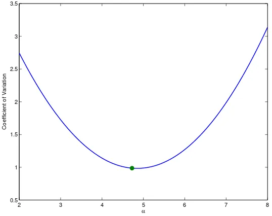
Having established that the two criteria will be asymptotically identical for truly rare events we now consider their performance with regard to variance reduction. To this end, for α ∈ _R define v(α) as the coefficient of variation of the IS estimator that uses drift θt = α(T −t). As illustrated in Figure 2.3 both ˆα and αe are very close

to the optimal value arg minα∈Rv(α), indicating that among all IS estimators using

(36)

1 1.1 1.2 1.3 1.4 1.5 1.6 1.7 1.8 1.9 1

2 3 4 5 6 7 8 9

c

α

GR Entropy

Figure 2.2: This figure compares the constantsαˆ, the slope of the linear drift selected by the GR criteria, andα_e, the slope selected by the entropy criteria, in the context of Example 2.3.1 b, aandT

are respectively 1.4, 0.25 and 1 in this example. As c varies along the horizontal axis here the probability_P(W ∈B) varies from0.5 to4.356×10−6_.

2 3 4 5 6 7 8

0.5 1 1.5 2 2.5 3 3.5

α

Coefficient of Variation

Figure 2.3: This figure illustrates a quadratic fit to the function v(α), wherev(α)is defined as the coefficient of the IS estimator for Example 2.3.1 that uses linear drift θt = α(T −t). Parameter values are c= 1.3869, b= 1.4, a = 0.25and T = 1 which leads to _P(RT

0 Wtdt∈B)≈0.0117. We

(37)

2.4 Functions of Extremes

In this section we return to the main problem and implement our two-stage IS al-gorithm for more general diffusions. In order to clearly demonstrate the utility of the second stage application we concentrate on functionals for which the first stage application is well-developed. In particular we restrict ourselves to functionals of the form

h(S) =f(ST, ST, ST)·1{ST<r, ST>`} =:h(ST, ST, ST),

where f :_R3 _7→

R is some function, and events of interest are of the form

Ba,b={x∈ C[0, T] : xT > a, xT <−b}

where a, b∈_R. We define B+

a =Ba,−∞ as the set of paths whose maximum exceeds

the level a and B_b− = B−∞,b is the set whose minimum is below −b. See Chen and

Huang (2012) for an elegant algorithm that can be used to implement the first stage of IS in this context.

Our estimator here is based on the fact that _E[h(ST, ST, ST)·1{S∈Ba,b}] is equal to

E[exp(A(WTθ))·Cˆφ(Wθ, N)·Λ−_θ1·g(W θ T, W

θ T, W

θ

T)·1{W∈BF(a),F(b)}],

whereg(w, w, w) =h(F−1₍_w₎_{, F}−1₍_w₎_{, F}−1₍_w_{)). When}_θ _{= 0 we refer to the resulting}

estimator as the “crude estimator”; in other words the crude estimator only involves the first stage application of IS and is not designed to address the rare event problem.

In order to implement this estimator one must be able to simulate

(38)

for an arbitrary set of times 0 < t1 < . . . < tn < T. This does not appear possible

for the optimal drift θ =h0 determined in Proposition 2.3.2 and so we must content ourselves with selecting piecewise constant drifts using Proposition 2.3.7.

In the remainder of this section we describe the zero-drift algorithm presented by Chen and Huang (2012) and show how it can be generalized to the case of piecewise constant drift. In principle this allows the user to implement the two-stage estimator using drifts that are arbitrarily close to the optimal drift θ =h0 determined in Proposition 2.3.2.

Zero Drift

When θt ≡ 0 we have Λ−1 = 1 and, given simulated Poisson event times 0 < t1 <

. . . < tn, we need only simulate

(WT, WT, Wt1, . . . , Wtn, WT).

One way to accomplish this is to first simulate the triplet (WT, WT, ξT), where ξT =

sup{t ∈ [0, T] : Wt = WT} is the temporal location of the maximum of W, and

then make use of the fact that conditional on this triplet the trajectory of W can be decomposed into two independent Brownian meanders (one on either side of ξT);

see Chen and Huang (2012) for a description. Skeletons of such processes can be simulated using results from Devroye (2009) and the minimum of a meander over [ti−1, ti], conditional on its values at the endpoints, can be simulated using the inverse

transform algorithm described at the end of Section 4.1 in Chen and Huang (2012). The global minimumW_T can then be determined from the local minima in the obvious way.

(39)

E provides a detailed outline of one such implementation. It follows the algorithm developed in Chen and Huang (2012) quite closely but uses a different method for simulating the triplet (WT, WT, ξT). In particular we generate the components of

this triplet in a different order; in Chen and Huang (2012) ξT is generated first using

inverse transform but it does not seem feasible to do so in the presence of drift, as such we generate the triplet in an order that is more amenable to the introduction of non-zero drift.

Remark 2.4.1. In the interest of computational efficiency Steps 4 to 12 in Algorithm

1 should only be performed if WT > F(a). This is because (i) generation of ξT uses

acceptance-rejection and (ii) generation of the local minima uses numerical inverse

transform. These steps can be expensive and therefore should only be carried out if

absolutely necessary.

Constant Drift

In this case we have, with an admitted abuse of notation, θt ≡ θ for some constant

θ ∈_R. Since Λθ = exp(−θWTθ +θ2T /2) it suffices to simulate

(Wθ_T, Wθ_T, W_tθ

1, . . . , W

θ tn, W

θ T).

In Appendix A we prove (see Theorem A.0.2) that the conditional law of Wθ, given the triplet (Wθ_T, W_Tθ, ξ_Tθ), does not depend on the value ofθ. Therefore if one is able to simulate the triplet one can then assume without loss of generality thatθ = 0 and proceed as in the case of zero drift by making use of independent meanders on either side of ξθ

T.

(40)

Piecewise Constant Drift

Here we fix a set of times 0 = s0 < s1 < . . . < sm = T and assume that θt takes

on the constant value θ(i) ∈ _R over the interval (si−1, si]; for completeness assume

θ0 = 0. The basic idea is to begin by creating m independent Brownian bridges by

first simulating (Wθ

s1, . . . , W

θ

sm). If one is then able to generate the maximum value

and its temporal location for each bridge (the temporal location of theith _{bridge will}

lie in [si−1, si]) then, since the law of theithbridge will not depend onθ(i), one can use

the decomposition into Brownian meanders over each subinterval [si−1, si]. A detailed

algorithm for implementing this procedure is provided in Algorithm 3.

2.4.1 Example - CIR Process With Large Maximum

In this example we illustrate how effective the second stage IS application can be when the event of interest is truly rare. In particular we compare the performance of the crude estimator (i.e. the IS estimator using only the first stage) to the two-stage estimator using constant drift and find that the latter performs admirably in cases where the former fails completely. We consider estimating

E[h(ST, ST, ST)·1{S∈B+a}] =E[h(ST, ST, ST)·1{ST>a}] (2.17)

where St denotes a so-called CIR process driven by the SDE

dSt =κ(α−St)dt+σ

p

StdWt, S0 =s0 ,

and we recall thath(s, s, s) is of the formf(s, s, s)·1{s>0} for some function f :R3 7→ R.

(41)

E[f(WT, WT, WT)·exp(A(WT))·Cˆφ(W, N)·1{WT>F(a), WT>F(0)}],

where F(x) = (2/σ)·(√x−√s0),

φ(x) = 1₂

4κα−σ2

2σ2₍_x₊₂√_s 0/σ) −

κ

2

x+2

√ s0

σ

2

− 4κα−σ2 2σ2₍_x₊₂√_s

0/σ)2 −

κ

2

,

and

A(x) = 4κα₂_σ−2σ2 log

x+2

√ s0 σ −κ 4

x+ 2

√ s0

σ

2

.

Ifais large then the event of interest{WT > F(a)}is rare and one might expect this

crude estimator to perform poorly.

The second stage application of IS is based on the fact that (2.17) is equal to

E[f(WθT, W θ

T, WTθ)·exp(A(WTθ))·Cˆφ(Wθ, N)·Λ−θ1·1{WTθ>F(a), WθT>F(0)}

]

and for our numerical example we use the constant drift

θ =T−1·_E[WT|WT > F(a)] =F(a)/T ,

which is the optimal constant drift according to our entropy-based optimality criteria (see Proposition 2.3.7).

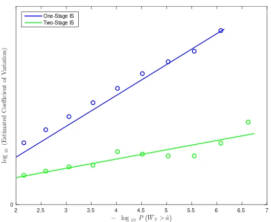
In Figure 2.4 we compare the performance of the two estimators in the case that

f(s, s, s) ≡ 1, which corresponds to simply estimating _P(ST > a). Ideally we could

plot the estimated coefficient of variation against_P(ST > a) asavaries, as this would

(42)

closed-form and is indicative of how rare the event of interest is. For each value of a in our grid the coefficient of variation is based on an independent sample of size 2·106 _with

λ= 10 (we found that using values ofλin excess of 10 did not appreciably impact the performance of the estimator but did increase CPU time substantially). We see that the two-stage IS procedure drastically outperforms the crude estimator and performs quite well in cases where the crude estimator fails completely, as it appears to occur for probabilities on the order of 10−6.

− log10P !

WT>ˆa"

2 2.5 3 3.5 4 4.5 5 5.5 6 6.5 7

lo

g1

0

(E

st

im

at

ed

C

o

e

ffi

ci

en

t

of

V

ar

ia

ti

on

)

One-Stage IS Two-Stage IS

Figure 2.4: Estimated coefficient of variation against _P(WT >aˆ) on the log scale. We are using 2,000,000 trajectories whenf(ST, ST, ST)≡1 with parametersσ= 0.15, κ= 0.5, α= 0.06, T = 1

and s0 = 0.06. We fit an exponential curve for the crude estimator and a linear curve for the

two-stage estimator (the two-stage estimator uses constant drift).

In Figure 2.5 we compare performance in the case that f(s, s, s) = s2, which corre-sponds to estimating _E[S_T2 ·1_{_S_T_>a_}]. The plot is produced in the same manner as Figure 2.4 and tells an identical story, namely that the addition of the second stage of IS allows the estimator to perform at an acceptable level of precision in cases where the crude estimator fails completely. Applying a second stage of Importance Sam-pling is almost cost free since we restricted ourselves to deterministic IS drifts and since sampling from (WT

θ

(43)

− log10 P !_WT_>

ˆ a"

2 2.5 3 3.5 4 4.5 5 5.5 6 6.5 7

lo

g1

0

(E

st

im

at

ed

C

o

e

ffi

ci

en

t

of

V

ar

ia

ti

on

)

0

One-Stage IS Two-Stage IS

Figure 2.5: Estimated coefficient of variation against P(WT >aˆ) on the log scale. We are using 2,000,000 trajectories whenf(ST, ST, ST) =S2T with parameters σ= 0.15, κ= 0.5, α= 0.06, T= 1ands0= 0.06. We fit an exponential curve and a linear curve for he First-Stage and the Two-Stage Importance Sampling estimator, respectively.

2.4.2 Example - OU Process With Large Maximum and Low

Minimum

In the previous example the optimal importance drift, when optimized over the whole of L2_[0_{, T}_{], is very nearly constant.} _{As such we were able to obtain substantial}

variance reduction using a very simple importance drift. In this section we consider an example where the optimal drift is non-linear in order to demonstrate the importance of selecting an importance drift that captures the salient features of the optimal (entropy-based) IS drift.

To this end we consider estimation of

E[h(ST, ST, ST)·1{S∈Ba,b}] =E[h(ST, ST, ST)·1{ST>a, ST<−b}], (2.18)

(44)

dSt=κ(α−St)dt+σdWt, S0 =s0.

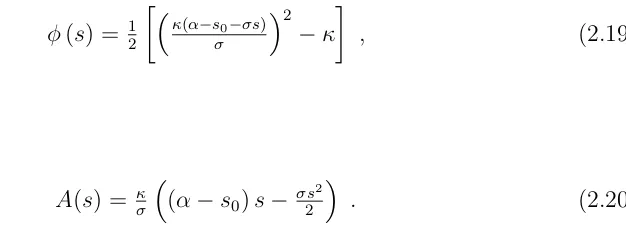
Since the boundaries±∞are unattainable here there is no implicit indicator inh. In this OU case we haveF(s) = (s−s0)/

√

σ,

φ(s) = 1₂

κ(α−s0−σs)

σ

2

−κ

, (2.19)

and

A(s) = _σκ(α−s0)s− σs 2

2

. (2.20)

We will compare the performance of three estimators - first is the crude estimator based only on the first stage application of IS, second is the two-stage estimator using constant drift θ = T−1 _·

E[WT|WT > a, WT <−b] and third is the two-stage

estimator using piecewise constant drift of the form

θt=t−11·E[Wt1|WT > a, WT <−b]·1{0<t≤t1}

+ (T −t1)−1·E[WT −Wt1|WT > a, WT <−b]·1{t1<t≤T} .

Motivated by the behaviour observed in Figure 2.1, in the case a > b we select t1 as

that point where ht attains its minimum value (in the case a < b) replace minimum

with maximum) and determine the temporal location of this minimum numerically.

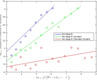
Figure 2.6 compares performance of the three estimators in the case thath(s, s, s)≡1, which corresponds to estimating _P(ST > a, ST < −b). As in the previous example

we plot the coefficients of variation against −log₁₀_P(WT > F(a), WT <−F(b)) for

(45)

In cases where _P(WT > F(a), WT <−F(b))<10

−6 _{we did not obtain a single}

infor-mative scenario using the crude estimator, and in cases where _P(WT > F(a), WT <

−F(b)) < 10−8 _{we did not obtain a single informative scenario using the two-stage}

estimator with constant drift. By contrast the two-stage estimator with piecewise constant drift performed quite well over the entire range.

− log10

1

P1WT>ˆa, WT<− ˆb 22

3 4 5 6 7 8 9

− lo g1 0 (E st im at ed C o e ffi ci en t of V ar ia ti on ) 1.4 1.6 1.8 2 2.2 2.4 2.6 2.8 3 3.2 One-Stage IS Two-Stage IS (Constant) Two-Stage IS (Piecewise Constant)

Figure 2.6: Estimated coefficient of variation versusP(WT >ˆa, WT <−ˆb)on thelogscale for the First-Stage estimator, Two-Stage estimator with constant drift and the Two-Stage estimator with piecewise constant drift. We fit an exponential curve for the First-Stage estimator and Two-Stage estimator with constant drift, and we fit a linear curve for the Two-Stage estimator with piecewise constant drift. The parameters used in this Figure areκ= 1, α= 0, σ=√2, s0= 0.06andT = 1.

The evidence here is consistent with that obtained in the previous example, namely that the two-stage estimator can perform well even when the crude estimator fails completely. However we also see that this performance boost is by no means guaran-teed, and we see that one must select an importance drift that is sufficiently reflective of ht.

(46)

computation time substantially since it increases the number of minima that have to be generated. If we have M subintervals and n trajectories, the Piecewise Constant Importance Sampling estimator will have to generate an extra 2n(M−1) minima on average. Therefore, it might be better to increase the number of simulations rather than adding subintervals. This tradeoff is problem-specific and depends highly on the shape of the minimum entropy drift. Consequently, one should analyze its behaviour before implementing the piecewise linear estimator.

2.5 Concluding Remarks

This chapter proposes an importance sampling procedure that can be used to estimate expectations of path functionals of diffusion processes that is free of discretization error and performs well when crude estimators fail completely. We pay particular at-tention to the so-called measure selection problem for standard Brownian motion and propose a simple criteria for selecting effective importance drifts for standard Brow-nian motion. The criteria is based on entropy minimization (between the importance measure and conditional law of the Brownian motion, given that its trajectory lies in some region of interest) and leads to an intuitive choice that is easy to implement. Moreover in the example considered in this paper the performance of importance sampling estimators based on this criteria is virtually indistinguishable from that of an alternative criteria, based on large deviations, that is known to be asymptotically optimal in a certain sense, but difficult to implement in practice.

(47)

development of algorithms that can be used for more general path functionals, a deeper understanding of the connection between our entropy criteria and the large deviations criteria proposed by Guasoni and Robertson (2008), as well as extending our approach to multivariate diffusions (where the Radon-Nykodym derivatives can be much more complicated to work with) and/or jump diffusions.

Bibliography

Søren Asmussen and Peter W. Glynn. Stochastic Simulation: Algorithms and Analy-sis. Springer, 1st edition, 2007.

Søren Asmussen, Dirk P. Kroese, and Reuven Y. Rubinstein. Heavy Tails, Importance Sampling And Cross–Entropy. Stoch. Models, 21:57–76, 2005.

Alexandros Beskos and Gareth O. Roberts. Exact Simulation of Diffusions. Ann.

Appl. Probab., 15(4):2422–2444, 2005.

Nan Chen and Zhengyu Huang. Brownian Meanders, Importance Sampling and Un-biased Simulation of Diffusion Extremes. Oper. Res. Lett., 40(6):554–563, 2012. Luc Devroye. On Exact Simulation Algorithms for Some Distributions Related to

Brownian Motion and Brownian Meanders, 2009.

Joe DiCesare. Imputation, Estimation and Missing Data in Finance. PhD thesis, University of Waterloo, 2006.

Joe DiCesare and Don McLeish. Simulation of Jump Diffusions and the Pricing of Options. Insurance: Mathematics and Economics, 43(3):316–326, 2008.

K. Giesecke and D. Smelov. Exact Sampling of Jump-Diffusions.Operations Research, 61(4):894–907, August 2013.

Paolo Guasoni and Scott Robertson. Optimal Importance Sampling With Explicit Formulas in Continuous Time. Finance Stoch., 12:1–19, 2008.

(48)

Chapter 3 Rare Event Simulation for

Portfolio Losses

3.1 Introduction

This chapter addresses the problem of estimating1

P(LN ≥x), (3.1)

whereLN is the loss on a portfolio ofN obligors andxis a large user-defined threshold.

The two primary means of estimating (3.1) in the conditional independence framework are convolution (see Merino and Nyfeler (2002)) and Monte Carlo. If N is large, as is often the case in practice, the former approach becomes unwieldy and the latter approach is the only feasible method. If in addition x is large, as the case when computing risk measures such as VaR or CVaR, the variability of the crude Monte Carlo estimator tends to be unacceptably large. If, as is so often the case in practice, the computational budget is limited then there is clear value in implementing variance reduction schemes.

Several authors have developed effective importance sampling (IS) algorithms for

(49)

mating (3.1) in particular models. At the present time, the most effective algorithms in the Gaussian and t models (assuming non-random loss given default, at least) are those developed by Glasserman and Li (2005) and Chan and Kroese (2010), respec-tively. This chapter develops a more general procedure that can be applied in a wide variety of models, including but not limited to the Gaussian and t. The proposed algorithm is more general, offers comparable performance when benchmarked against these “gold standards” (both of which are known to have good asymptotic proper-ties), requires approximately the same computation time as Glasserman and Li (2005) and requires substantially less computational time than the Chan and Kroese (2010) algorithm.

3.1.1 Summary of Proposed Algorithm

There are two components to any effective IS algorithm. The first is the identification of a parametric family of candidate measures from which to simulate. This family must be tractable in the sense that all members are straightforward to simulate from. The second is the criteria used to select an effective (in terms of variance reduction) member of the candidate family. In general this component involves both theoretical characterization of the optimal parameter value(s) and computational methods for approximating them.

(50)

function of the systematic factors) in the literature we term it a sequential exponential tilt in what follows. Exponential tilts are well known to provide very effective variance reduction in a wide variety of contexts (see Asmussen and Glynn (2007) and references therein) and the idea of using (what we call) sequential tilts in the portfolio problem has appeared elsewhere in the literature, most notably in Glasserman and Li (2005), albeit in less generality.

The second component of our algorithm consists of choosing the tilt parameters so as to ensure that the resulting IS measure has minimal Kullback-Liebler divergence (KLD) from the ideal (but impractical) zero-variance measure. In this sense our algorithm can be seen as a variant of the well-known cross-entropy (CE) method for estimating rare event probabilities. When combined with the parametric family described in the previous section this criteria allows one to characterize optimal pa-rameter values via intuitive moment-matching equations. Elementary properties of the parametric family ensure that these equations are well-behaved, and we exploit asymptotic features of the conditional independence structure to develop efficient ap-proximations to their solutions. In the homogeneous case the apap-proximations are available via simple quadrature, in more general cases efficient iterative algorithms (such as the adaptive CE algorithm described in Asmussen and Glynn (2007)) are available.

3.1.2 Brief Literature Review

(51)

For certain correlation structures the approach fails to be asymptotically optimal (but still seems to perform well in most cases of practical interest) and Glasserman et al. (2008) prove that asymptotic optimality can be achieved in these instances by using mixtures of sequential tilts. The only real drawback to the Glasserman and Li (2005) algorithm is that it is not clear how it could be extended to incorporate important phenomena such as heavy-tailed risk factors or correlation between default rates and loss given default.

At the present time the most effective available algorithm in the Studenttcopula case appears to be that of Chan and Kroese (2010), which combines conditional Monte Carlo with a clever observation regarding order statistics. The Chan and Kroese (2010) algorithms requires substantially less computational time than the algorithm developed by Bassamboo et al. (2006). The former algorithm is several times faster than the latter, and the algorithm proposed in this paper is several times faster than the former. The reason for this efficiency gain appears to be that Chan and Kroese (2010) requires one to sort high-dimensional vectors, which can be quite cumbersome when the number of obligors is large. In particular the complexity of the Chan and Kroese (2010) algorithm is of orderNlog(N) whereas the algorithm proposed in this paper is of order N.

Extensions of the Cross-Entropy Method with Applications to Diffusion Processes and Portfolio Losses

Scholarship@Western

Scholarship@Western

Extensions of the Cross-Entropy Method with Applications to

Extensions of the Cross-Entropy Method with Applications to

Diffusion Processes and Portfolio Losses

Diffusion Processes and Portfolio Losses

Applications to Diffusion Processes and

Portfolio Losses

Alexandre Scott

Graduate Program in Applied Mathematics

A thesis submitted in partial fulfillment

of the requirements for the degree of

Doctor of Philosophy

The School of Graduate and Postdoctoral Studies

Western University

London, Ontario, Canada

c

Table of Contents

List of Tables

List of Abbreviations, Symbols,

Nomenclature

Chapter 1

Introduction

1.1

The Cross-Entropy Method

Bibliography

Chapter 2

Rare Event Simulation for

Diffusion Processes

2.1

Introduction

2.1.1

Notation and Assumptions

2.2

Proposed Algorithm

2.2.1

First Stage Application - Discretization Error

2.2.2

Second Stage Application - Rare Event Problem

2.3

Rare Event IS for Brownian Motion

2.3.1

The Guasoni and Robertson (GR) Criteria

2.3.2

Entropy Minimization

2.3.3

Comparison Between Minimum Entropy and GR

2.4

Functions of Extremes

2.4.1

Example - CIR Process With Large Maximum

2.4.2

Example - OU Process With Large Maximum and Low

Minimum

2.5

Concluding Remarks

Bibliography

Chapter 3

Rare Event Simulation for

Portfolio Losses

3.1

Introduction

3.1.1

Summary of Proposed Algorithm

3.1.2

Brief Literature Review

3.1.3

Outline of the Chapter