https://doi.org/10.5194/nhess-19-2619-2019 © Author(s) 2019. This work is distributed under the Creative Commons Attribution 4.0 License.
Tsunami hazard and risk assessment for multiple buildings by
considering the spatial correlation of wave height using copulas
Yo Fukutani1, Shuji Moriguchi2, Kenjiro Terada2, Takuma Kotani3, Yu Otake4, and Toshikazu Kitano5
1College of Science and Engineering, Kanto Gakuin University, Yokohama, 236-8501, Japan 2International Research Institute of Disaster Science, Tohoku University, Sendai, 980-8572, Japan 3Research and Development Center, Nippon Koei Co., Ltd., Ibaraki, 300-1259, Japan
4Faculty of Engineering, Niigata University, Niigata, 950-2181, Japan 5Civil Engineering, Nagoya Institute of Technology, Nagoya, 466-8555, Japan
Correspondence:Yo Fukutani ([email protected]) Received: 27 April 2019 – Discussion started: 27 May 2019
Revised: 17 October 2019 – Accepted: 19 October 2019 – Published: 22 November 2019
Abstract.It is necessary to evaluate aggregate damage prob-ability to multiple buildings when performing probabilistic risk assessment for the buildings. The purpose of this study is to demonstrate a method of tsunami hazard and risk as-sessment for two buildings far away from each other, us-ing copulas of tsunami hazards that consider the nonlinear spatial correlation of tsunami wave heights. First, we sim-ulated the wave heights considering uncertainty by varying the slip amount and fault depths. The frequency distributions of the wave heights were evaluated via the response surface method. Based on the distributions and numerically simu-lated wave heights, we estimated the optimal copula via max-imum likelihood estimation. Subsequently, we evaluated the joint distributions of the wave heights and the aggregate dam-age probabilities via the marginal distributions and the esti-mated copulas. As a result, the aggregate damage probability of the 99th percentile value was approximately 1.0 % higher and the maximum value was approximately 3.0 % higher while considering the wave height correlation. We clearly showed the usefulness of copula modeling considering the wave height correlation in evaluating the probabilistic risk of multiple buildings. We only demonstrated the risk evalu-ation method for two buildings, but the effect of the wave height correlation on the results is expected to increase if more points are targeted.
1 Introduction
Probabilistic hazard and risk assessment methods of disasters are developed mainly in the field of nuclear safety focused on countermeasures relative to severe accidents at nuclear power plants. Among them, a variety of probabilistic tsunami hazard assessment (PTHA) and probabilistic tsunami risk as-sessment (PTRA) methods for tsunami disasters have been rapidly developed since the 2000s (e.g., Geist and Parsons, 2006; Annaka et al., 2007; González et al., 2009; Thio et al., 2010; Løvholt et al., 2012, 2015; Goda et al., 2014; Fuku-tani et al., 2015; Park and Cox, 2016; De Risi and Goda, 2017; Grezio et al., 2017; Davies et al., 2018). The main pur-pose of a PTHA is to assess the likelihood of a given mea-sure of tsunami hazard metrics (e.g., maximum tsunami wave height) being exceeded at a particular location within a given time period. The most basic outcome of such an analysis is typically expressed as a hazard curve, which shows the ex-ceedance level of the hazard metric with the probability. This is often expressed as a rate of exceedance per year. A PTHA can be expanded to a PTRA by combining hazard assess-ment with loss evaluation of a target. Several studies have proposed a method of PTRA for an individual site in a lo-cal area. Detailed risk assessment is undoubtedly important in terms of grasping the risk of exposing assets located in a local area.
Salgado-2620 Y. Fukutani et al.: Tsunami hazard and risk assessment for multiple buildings
Gálvez et al., 2014; Scheingraber and Käser, 2019). With re-spect to businesses that own a building portfolio, including factories and offices over a wide area, it is extremely im-portant in risk-based management decisions to evaluate the detailed risks posed by the building portfolio. A portfolio means a collection of assets held by an institution or a private individual. By quantitatively assessing the risks posed by the building portfolio, for example, it is possible to identify as-sets held that have a large impact on the overall risk and to compare the amount of risk held over time, which leads to support for decision-makers.
When evaluating physical risks for multiple buildings over a wide area, it is necessary to evaluate the aggregate risk for the buildings that are located at a distance. In these types of cases, it is necessary to evaluate the risk by considering the spatial correlation of hazards. For example, let us con-sider assessing the risk of two buildings located at two sites. When the positive correlation of hazards between two sites is strong, the hazard at one site tends to be large if the haz-ard at another site is large. In this case, the hazhaz-ards at the two target sites both increase, and as a result, the aggregate risk for the two buildings considering the hazard correlation increases. Conversely, when the positive correlation of haz-ards is small, the hazard at one site is not necessarily large, even if the hazard at another site is large. In this case, com-pared to the former case, the hazards at the two target sites are smaller, and as a result, the aggregate risk for the two build-ings is smaller if we assume that the vulnerability of the two buildings is equal. Therefore, analyses that do not consider the spatial correlation of hazards involve the risk of under-estimating the risk over a wide area. It is clear that the dif-ference of aggregate risk between two cases becomes more prominent as the number of target sites increases. Analyses that consider the spatial correlation of hazards are relatively advanced in the field of earthquake hazard and risk assess-ment (e.g., Boore et al., 2003; Wang and Takada, 2005; Park et al., 2007) albeit insufficient in the field of tsunami hazard and risk assessment. Analyses that consider the hazard cor-relation using copulas are used in hydrological/earthquake modeling (e.g., Goda and Ren, 2010; Goda and Tesfamariam, 2015; Salvadori et al., 2016) although there is a paucity of the same in tsunami modeling.
In this study, we assume the occurrence of a large earth-quake in the Sagami Trough in Japan that significantly af-fects the metropolitan area and evaluate the tsunami risk of two buildings located at distant locations by considering the spatial correlation of the tsunami wave height between the two sites. The objective of this study involves evaluat-ing the frequency distribution of the tsunami height via the response surface method and evaluating the spatial corre-lation of the tsunami heights and damages by using vari-ous copulas. Specifically, we analyze the frequency distri-bution (marginal distridistri-bution) of tsunami height via the re-sponse surface method and target two steel buildings located at Oiso and Miura along the Sagami Bay, Kanagawa
Prefec-ture, in Japan. Subsequently, we derive the joint distribution of tsunami wave heights between two sites by using various copulas and the marginal distributions, convert it to the joint distribution of damage by applying a damage function, and evaluate the expected value of the aggregate damage proba-bility for the target buildings. Finally, we confirm the extent to which the expected value of the aggregate damage prob-ability fluctuates in a case where the spatial correlation of tsunami wave height is considered and a case where it is not considered.
Section 2 provides an outline of the response surface method and tsunami hazard and risk assessment method for multiple buildings using copulas. Section 3 describes a case where the proposed method is applied to the Sagami Trough area. The final conclusions are discussed in Sect. 4.
2 Methodology
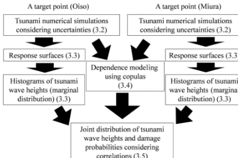
Figure 1 shows a flowchart of tsunami hazard and risk assess-ment considering the correlation of tsunami wave heights in this study. Herein, the risk assessment target points only cor-respond to two points: Oiso and Miura, Kanagawa Prefec-ture, in Japan. Figure 2 shows the location of these points. First, we simulate the tsunami wave heights considering the uncertainty at the target sites by numerical tsunami simu-lations via nonlinear long-wave equations. Based on this, we construct a response surface and apply probability distri-butions to obtain a frequency distribution of tsunami wave heights. This distribution becomes a marginal distribution for a joint distribution of tsunami wave heights of two tar-get points. Separately, we estimate appropriate copula via maximum likelihood estimation from the simulation results of the tsunami wave height considering uncertainty. Sub-sequently, we obtain a joint distribution of tsunami wave heights from the estimated copula and the marginal distribu-tions of tsunami wave height. Furthermore, we obtain a joint distribution of damage probabilities by applying the tsunami damage function.
The outline of the response surface method and copula modeling used in this study is explained below. The response surface method is a statistical combination method to de-termine an optimum solution using the lowest number of measurement data possible. The basic idea is based on a reliability-based design scheme developed in the research field of geomechanics (e.g., Honjo, 2011). Generally, the re-sponse surface model is given by Eq. (1) as follows:
y=f (x1, x2, . . ., xn)+ε, (1)
in-Figure 1. Flowchart of probabilistic tsunami hazard and risk as-sessment considering the spatial correlation of tsunami wave height. Numbers in the parentheses indicate the section numbers escribed.
undation height and flow depth variability, but such an anal-ysis is outside the scope of this study. Tsunami hazard as-sessment has many uncertainties in each process of tsunami generation, propagation, and run-up. Even considering only the earthquake source parameters that are the basis for cal-culating the initial displaced water level of the tsunami, there are fault length, fault width, fault depth, slip amount, rake, strike, and dip. The temporal and spatial changes of all these parameters more or less affect the tsunami hazard assess-ment. Numerous studies on the effect of earthquake source parameters on the initial displaced water level of tsunamis have been conducted (e.g., Hwang and Divoky, 1970; Ward, 1982; Ng et al., 1991; Pelayo and Wiens, 1992; Whitmore, 1993; Geist and Yoshioka, 1996; Geist, 1999, 2002; Song et al., 2005). These studies reported that fault slip was an im-portant factor governing tsunami intensity. In addition, the Sagami Trough, which is the target earthquake of this study, has a complex crustal structure in the area where the Pa-cific Plate, the Philippine Sea Plate, and the North American Plate meet. Therefore, the depth where the Sagami Trough earthquake occurs is considered uncertain. Therefore, in this study, we decided to consider only the tsunami hazard uncer-tainty caused by the changes of slip amount and fault depth as an example. The heterogeneity of fault slip is an equally important factor, but we did not consider nonuniform slip distribution for purposes of simplicity. It is an important is-sue in the future to evaluate the heterogeneity of fault slip using response surface methodology. This is true for both slip heterogeneity and other fault parameters. For the above reasons, we model maximum tsunami wave height consider-ing tsunami wave uncertainty with Eq. (2) after conductconsider-ing a tsunami numerical simulation with a nonlinear long-wave equation. This formula is following the tsunami hazard eval-uation method proposed by Kotani et al. (2016) that applied a reliability analysis framework using the response surface
method proposed in Honjo (2011). The expression is as fol-lows:
h(S, D)=aS+bD+cSD+dS2+e, (2)
whereh(S,D)denotes the tsunami wave height;Sdenotes the slip;Ddenotes the fault depth; anda,b,c,d, andedenote the undetermined coefficients. It should be noted that an error term is not included in Eq. (2). An example of the error term is to consider an error due to modeling. For example, Kotani et al. (2016) quantified the modeling error as the difference between the observed tsunami height and the numerically simulated tsunami height. The modeling error of the numeri-cal analysis was also considered as one of the tsunami hazard uncertainties. However, the main purpose of this study is to propose a tsunami damage assessment method for multiple buildings using a copula considering wave height correlation. Therefore, the modeling error is also ignored for simplifica-tion in this study.
This response surface method has an advantage that the probability distribution of the objective variable can be eas-ily evaluated by applying an appropriate probability distri-bution to the explanatory variable and performing a Monte Carlo simulation. Although the tsunami numerical simula-tion considering uncertainty usually has a high calculasimula-tion cost to conduct vast numbers of simulation cases, it is pos-sible to significantly reduce the simulation cost by using the response surface method.
The foundation of the copula theory corresponds to the Sklar theorem (Sklar, 1959). A copula is a multivariate dis-tribution whose marginals are all uniform over [0, 1]. Given this in combination with the fact that any continuous random variable can be transformed to be uniform over [0, 1] by its probability integral transformation, copulas are used to sep-arately provide multivariate dependence structure from the marginal distributions. LetF be an-dimensional distribution function with marginalsF1, . . . ,Fn andH be a joint distri-bution function. There exists an-dimensional copulaCsuch that for allx in the domain of F, the following expression holds (Sklar, 1959):
H (x1, . . ., xn)=C{F1(x1) , . . ., Fn(xn)} =C (u1, . . ., un), (3) whereui=Fi(xi)∈ [0, 1], i=1, . . . ,n. Figure 3 shows a simple synthetic example of a copula in a bivariate case. Fig-ure 3a is a joint distribution function, Fig. 3b and c are dis-tribution functions of each variable (marginal disdis-tributions), and Fig. 3c is a copula distributed over [0, 1]. Joe (1997) and Nelsen (1999) proposed the two comprehensive treatments on the topic. The two most common elliptical copulas corre-spond to the Gaussian copula and thet copula whose copula functions in the bivariate case correspond to Eqs. (4) and (5).
C (u1u2)=86
8−1(u1) , 8−1(u2)
2622 Y. Fukutani et al.: Tsunami hazard and risk assessment for multiple buildings
Figure 2. (a)Major subduction-zone earthquakes around the Japanese islands including the Sagami Trough earthquake, the Nankai Trough
earthquake, and the Tohoku-type earthquake (yellow area);(b)two targets points, Oiso and Miura, Kanagawa Prefecture, for tsunami hazard
and risk assessment.
Figure 3.A simple synthetic example of a copula in a bivariate case.(a)Joint distribution;(b, c)are distribution functions of each variable
(marginal distribution) and(d)is a copula distributed over [0, 1].
C (u1u2)=t6,ν
tν−1(u1) , tν−1(u2)
(5) The Gaussian copula is simply derived from a multivariate Gaussian distribution function86with mean zero and corre-lation matrix6by transforming the marginals by the inverse of the standard normal distribution function8. Given a mul-tivariate centeredt-distribution functiont6,νwith correlation
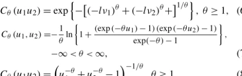
Cθ(u1u2)=exp
n
−(−lν1)θ+(−lν2)θ+
1/θo
, θ≥1, (6) Cθ(u1, u2)=−
1 θln
1+(exp(−θ u1)−1) (exp(−θ u2)−1) exp(−θ )−1
,
−∞< θ <∞, (7)
Cθ(u1u2)=
u−θ1 +u−θ2 −1 −1/θ
, θ≥1. (8)
The Gumbel and Clayton copulas capture upper tail de-pendence and lower tail dede-pendence, respectively, while the Frank copula does not exhibit tail dependence. Specifically,
θis estimated based on the maximum log-likelihood method. The copulas denote the symmetrical property with respect to diagonal lines of a unit square. To handle asymmetrical data in transformed space, we used an asymmetrical extreme-value copula (Tawn, 1988; Genest and Favre, 2007; Genest and Segers, 2009). Extreme-value copulas are characterized by the dependence functionAas given in Eq. (9):
C (u1, u2)=exp
log(u1u2) A
log(u
1)
log(u1u2)
. (9)
An asymmetric model using the copula with three parameters as mentioned by Tawn (1988) is given by
A(t )=θr(1−t )r+ϕrtr 1/r+(θ−ϕ)t+1−θ, (10) wherer,θ, andϕare estimated based on the maximum log-likelihood method. The special case θ=1 andϕ=1 corre-sponds to the symmetric model proposed by Gumbel (1960), and thus this is termed as the asymmetric Gumbel copula. We use this copula for modeling asymmetrical data dependence. In this study, we use the bivariate case as the tsunami wave height at two target points and model the correlation using a copula. The linear correlation coefficient (Pearson’s correla-tion coefficient) is an index that captures the linear relacorrela-tion between variables and essentially cannot express the depen-dency between variables that are not in linear relation. Con-versely, the copula is a function that expresses the correlation based on the order of the data of each variable rather than the data themselves. The order of the data is expressed by Kendall’sτ (Kendall, 1938). Therefore, it is possible to quan-tify the nonlinear correlation between the variables. Table 1 shows theoretical value of Kendall’sτ corresponding to the bivariate copulas and their parameter vectors. In this study, we show a simple evaluation method for two target points, although correlation between more points can be considered by using copulas.
3 Application to the Sagami Trough area
In this chapter, we demonstrate a case study where the hazard and risk assessment method described in the previous chapter is applied for two buildings located on the coast of Sagami Bay, Kanagawa Prefecture, in Japan. Section 3.1 shows the
Table 1.Bivariate copula, parameter vectors, and Kendall’sτ.
Copula Parameter Kendall’sτ
Gaussian copula ρ (2/π )arcsinρ tcopula ρ,ν (2/π )arcsinρ Clayton copula θ θ/(θ+2)
Frank copula θ 1−4/θ+4D1(θ )/θ Gumbel copula θ 1−1/θ
Asymmetric Gumbel copula r,θ,ϕ
1
R
0
t (1−t )A00(t )
A(t ) dt
ρ: Pearson’s correlation coefficient;D1(θ )= θ
R
0
x θ
(ex−1)dx: the first Debye function.
assessment target points, Sect. 3.2 shows the tsunami nu-merical simulation considering uncertainties, Sect. 3.3 con-structs the response surface, Sect. 3.4 shows the modeling of tsunami wave height correlation using copulas, and Sect. 3.5 shows the results of the evaluation and discussion.
3.1 Risk assessment targets
Figure 2a shows major subduction-zone earthquakes around the Japanese islands, namely the Sagami Trough earthquake, the Nankai Trough earthquake, and the Tohoku-type earth-quake announced by NIED (2017). Figure 2b shows the lo-cated points of tsunami hazard and risk assessment targets, namely Oiso and Miura, Kanagawa Prefecture, in Japan. The Sagami Trough earthquake covers most of the Kanto region, including the target points. Oiso is located at the approximate center of Sagami Bay coast, and Miura is located at the tip of the Miura Peninsula, which is located between Tokyo Bay and Sagami Bay. We assume a steel-framed building located at these two points and evaluate the tsunami damage proba-bility for the two buildings.
3.2 Tsunami numerical simulation considering uncertainties
In this section, we evaluate the tsunami wave heights by con-sidering the uncertainty at the target points.
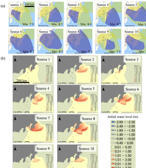
We selected 10 earthquake occurrence sources of the mo-ment magnitude (Mw) 8 class along the Sagami Trough,
which significantly affect the metropolitan area in Japan. The Sagami Trough is a 300 km long boundary between the Philippine Sea and North American plates. The assumed earthquake sources are shown in Fig. 4a. There are 10 earth-quake sources, and theMwof the sources ranges fromMw=
7.9 to Mw=8.6. Source 8 has maximum Mw=8.6. The
2624 Y. Fukutani et al.: Tsunami hazard and risk assessment for multiple buildings
Figure 4. (a)The 10 sources of the Sagami Trough earthquakes (NIED, 2017) and(b)initial water levels of the tsunami calculated from
Table 2.Moment magnitude, average slip, number of faults, and area in each earthquake source of the Sagami Trough earthquake.
Source Moment Average Number Area
number magnitude slip of faults (km2)
(Mw) (m)
1 7.9 2.5 1207 7544
2 8.2 4.0 2392 14 950
3 8.0 2.7 1533 9581
4 8.3 4.6 3393 21 206
5 8.4 5.0 3599 22 494
6 8.5 5.8 4926 30 788
7 8.5 5.2 4822 30 138
8 8.6 6.3 6149 38 431
9 7.9 2.5 1234 7713
10 8.2 3.0 2825 17 656
square, and the slip amount of the fault was set to a uniform value based on the moment magnitude (Mw) of each
earth-quake by using the following scaling laws of earthearth-quakes ac-cording to Kanamori (1977):
Mo=µSA, (11)
Mw=
log10Mo−9.1
1.5 , (12)
where “Mo” denotes moment magnitude (Nm), µ denotes shear modulus (Pa), S denotes slip amount (m), andA de-notes earthquake source area (m2). µ was set to 3.4× 10¹⁰(Pa). In this study, we did not consider nonuniform slip distribution for purposes of simplicity. We set other fault pa-rameters (i.e., fault depth, dip, rake, and strike) to the sources based on information published by the Cabinet Office (2013) in Japan, which were created from the crustal structure of data of the plates.
Figure 4b shows the calculation results of the initial wa-ter level distribution of the tsunami using the Okada (1985) equation. The initial water level of up to approximately +3.5 m is distributed off to Sagami Bay and Tokyo Bay. Us-ing the initial water level as an input value, we performed a tsunami numerical simulation via a nonlinear long-wave equation. We use the following continuity equation (Eq. 13) and nonlinear shallow water equations (Eqs. 14 and 15) as follows:
∂η ∂t +
∂M ∂x +
∂N
∂y =0, (13)
∂M ∂t +
∂ ∂x
M2 D
+ ∂
∂y
MN
D
+gD∂η ∂x
+ gn
2 D7/3M
p
M2+N2=0, (14)
∂N ∂t +
∂ ∂x
MN
D
+ ∂
∂y
N2 D
+gD∂η
∂y (15)
+ gn
2 D7/3N
p
M2+N2=0, (16)
whereη denotes the water level,D denotes the total water level, g denotes the acceleration due to gravity,n denotes the Manning coefficient, andMandN denote the fluxes in thexandydirections, respectively. The governing equations were discretized via the staggered leapfrog scheme (Goto and Ogawa, 1982; UNESCO, 1997). To consider wave height uncertainty, we implemented 25 cases of tsunami numerical simulation for each earthquake source. As detailed in the sec-ond chapter, this study focused on the slip amount and the fault depth among many uncertain factors. In each source, the slip amount was varied by±0.1 times and±0.05 times with respect to the reference case (five cases) in terms of
Mwconversion based on the scaling law, and the fault depth
was changed by+2.0,+1.0,−0.5, and−1.0 km with respect to the reference case (five cases) to consider the changes of the slip and the fault depth as uncertainty.
There are a total of 10 earthquake sources; thus, we imple-mented a total of 250 cases of tsunami numerical simulation nested in four stages of 270, 90, 30, and 10 m in the Japanese plane rectangular coordinate system IX for each simulation and executed the simulation for 3 h from the earthquake oc-currence. As an example, Fig. 5 shows the numerical simu-lation results of nine cases around Oiso and Miura in which theMw of source 8 is changed to±0.1 and the fault depth
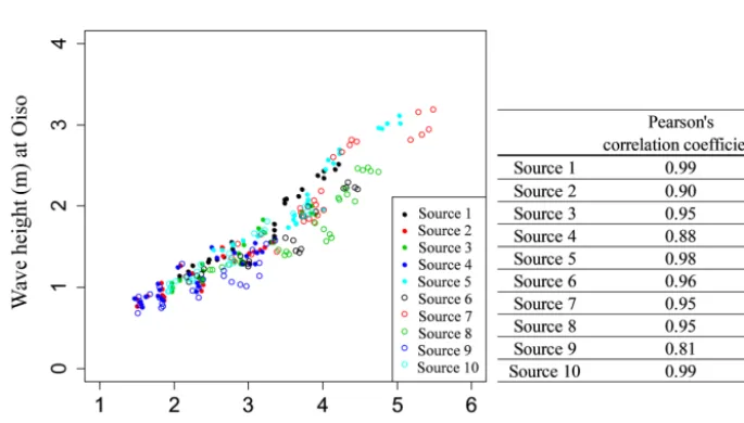
is changed to+2.0 and−1.0 km. As shown in the figure, the distributions of the maximum tsunami wave height vary lo-cally by changing the slip amount and the fault depth, and the effect of the slip amount on the maximum tsunami wave height is more dominant than the fault depth. In addition, while there is a clear positive correlation between the maxi-mum tsunami wave height and slip amount of the earthquake, there is no clear correlation between the maximum tsunami wave height and the fault depth. Figure 6 shows the maxi-mum tsunami wave heights of Miura and Oiso and Pearson’s correlation coefficient relative to the tsunami numerical sim-ulation results of each earthquake source. We confirmed that the correlation coefficient corresponded to at least 0.8 in any source; thus the correlation between tsunami wave height of Miura and Oiso was relatively high. The results suggest that we should assess tsunami risk considering the spatial corre-lation of tsunami wave height between the target points. 3.3 Construction of response surface
In this section, we construct response surfaces, which indi-cate maximum wave height at target sites.
2626 Y. Fukutani et al.: Tsunami hazard and risk assessment for multiple buildings
Figure 5.Tsunami numerical simulation results (aOiso andbMiura) in the case changing theMw(moment magnitude) and the fault depth
of source 8.
Figure 6.Maximum tsunami wave heights simulated from the tsunami numerical simulation at Miura and Oiso and Pearson’s correlation
coefficients in each earthquake source.
fault depth, and the objective variable denotes the maximum wave height at the target sites. We performed the regression analysis based on all combinations of four explanatory vari-ables (24−1=15 cases) and adopted a response surface with a high coefficient of determination and the minimum Akaike information criterion (AIC) (Akaike, 1974). AIC can
Figure 7.Response surfaces at(a)Oiso and(b)Miura for source 8 of the Sagami Trough earthquake. The blue circle denotes the maxi-mum wave height obtained from the tsunami numerical simulations, and the red curved surface denotes the response surface.
example, Fig. 7a and b show the response surface for the earthquake source 8 (Mw=8.6) with the highestMw in the
Sagami Trough earthquake. The blue circle denotes the max-imum wave height obtained from the tsunami numerical sim-ulations, and the red curved surface denotes the response sur-face. The response surfaces accurately represented the results of the tsunami numerical simulation. The response surfaces are in accordance with Eq. (16) for Oiso and Eq. (17) for Miura as follows:
h(S, D)=0.6567S+0.0459D−0.5189S2+0.5147, (17)
h(S, D)=11.1136S−4.0165S2−3.1327. (18) We can obtain the frequency distribution of the tsunami wave height by giving a probability distribution function that ex-presses the uncertainty in the explanatory variable (slip ra-tio S and fault depth D) of the evaluated response surface and by performing a Monte Carlo simulation.
As reported by Japan Society of Civil Engineers (2002), the estimated variation ofMwof an earthquake of the same
magnitude is approximately 0.1. Based on the aforemen-tioned value, we set a normal distribution with an average value of 1.0 and a standard deviation of 0.1 for the slip rate by using the scaling law. With respect to the uncertainty of the fault depth, we also set a normal distribution. The aver-age value was set to 0.0 m, and the standard deviation was set to a random number generated from a lognormal distri-bution that was obtained from the seismic observation error data from October 2016 to September 2017 (N=305 030) as published by the Japan Meteorological Agency (2017). We used the lognormal distribution with an average of 0.12 km and a standard deviation of 0.65 km. We would like to note that it is essentially necessary to apply a probability distribu-tion that appropriately expresses all possible uncertainties to the explanatory variables of the response surface, but in this study we applied a relatively limited probability distribution as uncertainty since we did not focus on discussing the details of the tsunami wave uncertainty but on the proposed tsunami
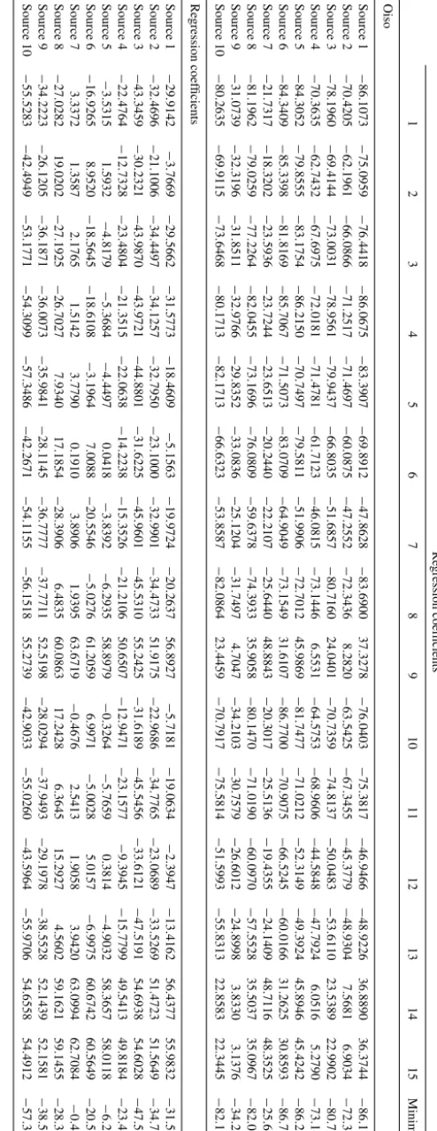
hazard and risk assessment method using response surface and copulas. Figure 8a and b show the frequency distribu-tion of the tsunami wave height obtained by the aforemen-tioned procedure. By using the response surface method, we can significantly reduce the simulation costs for probabilistic tsunami hazard assessment considering uncertainty.
To ascertain the normality of the frequency distributions, we performed the Kolmogorov–Smirnov test. Table 5 shows the results ofpvalues for each source. In several cases the
pvalues were less than 0.05, thereby indicating that the dis-tribution of the tsunami heights does not necessarily follow a normal distribution.
3.4 Dependence modeling using copulas
In this section, we estimate appropriate copulas from the re-sults of the tsunami numerical simulation considering un-certainties and evaluate the spatial correlation structure of tsunami wave height between two sites.
As confirmed in the previous section, despite the high lin-ear correlation of the frequency distribution of the tsunami wave height in Miura and Oiso, it is observed that the nor-mality of tsunami wave height for several sources was not secured by the normality test. The Pearson correlation coeffi-cient did not accurately grasp the spatial correlation structure of tsunami wave height, and thus we attempt modeling using a copula. Hereafter, we only illustrate the analysis results of the earthquake source 8 (Mw=8.6) with the largestMw as
an example.
Figure 8.Histograms of tsunami wave height simulated from the response surface at(a)Oiso and(b)Miura for source 8 of the Sagami Trough earthquake.
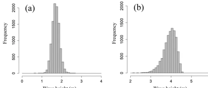
Table 4.Regression coefficients of each selected response surface
for each earthquake source.
Regression coefficients
a b c d e
Oiso
Source 1 1.1705 0.1039 −0.0371 0.3051 0.1927
Source 2 0.9868 0.0598 0.0000 0.0000 0.1037
Source 3 1.3747 0.0566 0.0000 0.0000 0.0040
Source 4 0.9568 0.0625 0.0000 0.0000 0.1184
Source 5 0.7991 0.0592 0.0000 0.6449 0.6303
Source 6 0.0000 0.0404 0.0000 0.7610 0.7538
Source 7 2.2360 0.0445 0.0000 0.0000 −0.0971
Source 8 0.6567 0.0459 0.0000 0.5189 0.5147
Source 9 0.0000 0.0661 0.0000 0.3945 0.5739
Source 10 −1.3690 −0.0972 0.0423 0.0000 −0.0029
Miura
Source 1 6.2764 0.0832 0.0000 −1.7394 −1.3700
Source 2 2.3946 0.0000 −0.0336 0.0000 −0.1281
Source 3 2.5601 0.0000 0.0000 0.0000 0.2187
Source 4 3.8893 0.0000 −0.0767 −0.7610 −0.8384
Source 5 2.6802 0.0643 0.0000 0.0000 1.0744
Source 6 8.0738 0.0000 0.0000 −2.5004 −2.1023
Source 7 0.0000 0.0829 0.0000 1.3910 2.4982
Source 8 11.1136 0.0000 0.0000 −4.0165 −3.1327
Source 9 2.4222 0.0000 0.0000 0.0000 −0.1673
Source 10 −2.5917 −0.1083 0.0869 0.0000 −0.1061
copula. By considering the spatial correlation of the tsunami wave heights using copula, we performed a Monte Carlo sim-ulation that appropriately captures the nonlinear spatial cor-relation of the tsunami wave height. We clearly showed the usefulness of copula modeling considering the wave height correlation.
Table 7 shows the result of estimating copulas under the same procedure for other earthquake sources. In the earth-quake sources targeted in this study, four types of copula were estimated, namely the rotated Gumbel copula, asym-metric Gumbel copula, Frank copula, and Gumbel copula.
Table 5.Kolmogorov–Smirnov test results.
pvalue
Oiso Miura
Source 1 0.00 0.00
Source 2 0.00 0.89
Source 3 0.00 0.61
Source 4 0.00 0.15
Source 5 0.07 0.95
Source 6 0.72 0.02
Source 7 0.79 0.50
Source 8 0.26 0.00
Source 9 0.00 0.93
Source 10 0.03 0.97
Figure 9.Selected Frank copula for source 8.
2630 Y. Fukutani et al.: Tsunami hazard and risk assessment for multiple buildings
Figure 10. Empirical cumulative distributions of tsunami wave
height (aOiso andbMiura) for source 8.
Table 6.Maximum likelihood estimation results of each copula for
source 8.
Name of copulas Log-likelihood AIC BIC
Gaussian copula 24.72 −47.43 −46.21
tcopula 24.62 −45.23 −42.79
Clayton copula 24.46 −46.93 −45.71
Gumbel copula 20.03 −38.06 −36.84
Frank copula 26.16 −50.33 −49.11
Rotated Clayton copula 14.53 −27.06 −25.84
Rotated Gumbel copula 25.77 −49.54 −48.32
Asymmetric Gumbel copula 19.90 −35.80 −33.36
Rotated asymmetric Gumbel copula 25.69 −47.38 −44.94
under the effects from the relative position of the earthquake sources and the target points, the bottom and land topogra-phy.
3.5 Risk assessment results and discussion
In this section, we evaluate the joint distribution of tsunami wave heights and damage probability of target buildings for the entire area of the Sagami Trough earthquake using the occurrence probability weights of each earthquake source.
Table 8 shows the occurrence probability weights of each source of the Sagami Trough earthquake published by NIED (2017). We first determine the earthquake occur-rence source via uniform random numbers using the weights and then evaluate the joint distribution of the tsunami wave heights due to the determined earthquake using the estimated copula. Figure 13 shows the results of evaluation by Monte Carlo simulation with 10 000 trials. Figure 13a shows the joint distribution of the tsunami wave heights considering the spatial correlation of the wave height, and Fig. 13b shows the results without considering the spatial correlation of the tsunami wave height. Furthermore, Fig. 13c shows the joint damage probability of two buildings that transform both axes of tsunami wave heights in Fig. 13b into the damage proba-bility by using the damage function of the steel frame (Sup-pasri et al., 2013) based on the assumption that a steel build-ing exists at the evaluation target point. Table 9 shows the av-erage value of the aggregate damage probability of two build-ings, 95th percentile value, 99th percentile value, and
maxi-Table 7. Estimated optimal copulas, copula parameters, and
Kendall’sτfor each source of the Sagami Trough earthquake.
Estimated copulas Parameters Kendall’sτ
Source 1 rotated Gumbel copula 20.42 0.95
Source 2 asymmetric Gumbel copula 1.00, 5.08, 0.85 0.70
Source 3 rotated Gumbel copula 4.62 0.78
Source 4 Frank copula 10.54 0.68
Source 5 rotated Gumbel copula 9.24 0.89
Source 6 Frank copula 22.11 0.83
Source 7 Gumbel copula 5.68 0.82
Source 8 Frank copula 17.77 0.80
Source 9 Gumbel copula 2.87 0.65
Source 10 Frank copula 35.76 0.89
Table 8. Occurrence probability weights of each source of the
Sagami Trough earthquake (NIED, 2017).
Occurrence probability weights
Source 1 0.37
Source 2 0.06
Source 3 0.30
Source 4 0.05
Source 5 0.03
Source 6 0.01
Source 7 0.01
Source 8 0.02
Source 9 0.11
Source 10 0.04
Summation 1.00
mum value assuming that the two buildings exhibit the same asset value. Although the expected value of the aggregate damage probability barely changed when compared with that of the no-correlation case, the aggregate damage probability of the 99th percentile value was approximately 1.0 % higher and the maximum value was approximately 3.0 % higher when considering the hazard correlation utilizing the copu-las. We clearly showed the significance of considering the spatial correlation structure of tsunami wave height in evalu-ating tsunami risks for a building portfolio. In this study we only demonstrated the evaluation method for two points, but the effect of the wave height correlation on the evaluation result is expected to increase if more points are targeted.
4 Conclusion
as-Figure 11.Monte Carlo simulation results for source 8. The black points denote the results with 10 000 trials(a)considering and(b)not considering the spatial correlation of tsunami wave heights using the Frank copulas. The red points denote the results calculated from 25 cases of tsunami numerical simulation.
Figure 12.Estimated optimal copulas distributed on [0, 1]2with 10 000 trials.(a)Rotated Gumbel copula for source 1,(b)asymmetric
Gumbel copula for source 2,(c)rotated Gumbel copula for source 3,(d)Frank copula for source 4,(e)rotated Gumbel copula for source 5,
(f)Frank copula for source 6,(g)Gumbel copula for source 7,(h)Frank copula for source 8,(i)Gumbel copula for source 9, and(j)Frank
copula for source 10.
Table 9.Tsunami risk assessment results.
Aggregate damage probability of the two buildings
No correlation (A) Correlation (B) Difference (B−A)
Average 58.8 % 58.8 % 0.0 %
95th percentile 66.2 % 67.0 % 0.9 %
99th percentile 68.9 % 69.7 % 0.8 %
Maximum 73.5 % 76.7 % 3.1 %
ex-2632 Y. Fukutani et al.: Tsunami hazard and risk assessment for multiple buildings
Figure 13. (a)Joint distribution of tsunami wave height considering wave height correlation and(b)not considering wave height correlation.
(c)Joint damage probability for the all sources of the Sagami Trough earthquake. The black points denote the Monte Carlo simulation results
with 10 000 trials, and the red points denote the results simulated via tsunami numerical simulations.
ists. In addition, the response surface method used in this study significantly reduces the numerical simulation costs for probabilistic tsunami hazard assessment considering uncer-tainty. In this study, we only focused on the slip amount and fault depth among many tsunami hazard uncertainties, and we evaluated them using the response surface method. It has been reported that the heterogeneity of the slip distribution of the fault has a great influence on tsunami intensity. It is a future issue to evaluate these effects with a response surface method.
The evaluation result was shown for only two buildings, but when an entity evaluates the risk of assets it owns it is assumed that there will be more target sites. It is clear that as the number of target assets increases, the percentile value and maximum value of the aggregate damage of assets become more prominent. Risk assessment that does not consider the spatial correlation of wave heights will lead to the underes-timation of the risks held. The basic method shown in this study can be applied even when the number of target assets
increases. It is also important to avoid underestimating the assessed risk by considering the wave height correlation us-ing a copula. It is expected that the tsunami risk assessment method for a building portfolio over a wide area as proposed in this study can be used for probabilistic tsunami risk assess-ment of real-estate portfolios or business continuity plans by parties such as large companies, insurance companies, and real-estate agencies.
Data availability. The earthquake source parameters of the Sagami Trough model used in this study are freely available at http:// www.j-shis.bosai.go.jp/map/JSHIS2/download.html?lang=en (last access: 21 November 2019; National Research Institute for Earth Science and Disaster, 2019).
Competing interests. The authors declare that they have no conflict of interest.
Acknowledgements. We thank two reviewers who provided us valu-able comments and helped improve the manuscript. This research was partially supported by funding from the International Research Institute of Disaster Science (IRIDeS) at Tohoku University.
Financial support. This research has been supported by the Inter-national Research Institute of Disaster Science (IRIDeS) at Tohoku University (Tsunami mitigation research 2).
Review statement. This paper was edited by Ira Didenkulova and reviewed by Elena Suleimani and one anonymous referee.
References
Akaike, H.: A new look at the statistical model
iden-tification, IEEE T. Automat. Control, 19, 716–723,
https://doi.org/10.1109/TAC.1974.1100705, 1974.
Annaka, T., Satake, K., Sakakiyama, T., Yanagisawa, K., and Shuto, N.: Logic-tree Approach for Probabilistic Tsunami Hazard Anal-ysis and its Applications to the Japanese Coasts, Pure Appl. Geo-phys., 164, 577–592, https://doi.org/10.1007/s00024-006-0174-3, 2007.
Boore, D. M., Gibbs, J. F., Joyner, W. B., Tinsley, J. C., and Ponti, D. J.: Estimated ground motion from the 1994 Northridge, California, earthquake at the site of the interstate 10 and La Cienega Boulevard bridge collapse, West Los Ange-les, California, Bull. Seismol. Soc. Am., 93, 2737–2751, https://doi.org/10.1785/0120020197, 2003.
Cabinet Office: The study meeting for the Tokyo Inland Earth-quakes, available at: http://www.bousai.go.jp/kaigirep/chuobou/ senmon/shutochokkajishinmodel/ (last access: 11 May 2018), 2013.
Chang, S. E., Shinozuka, M., and Moore, J. E.: Probabilistic earthquake scenarios: Extending risk analysis methodologies to spatially distributed systems, Earthq. Spect., 16, 557–572, https://doi.org/10.1193/1.1586127, 2000.
Davies, G., Griffin, J., Løvholt, F., Glimsdal, S., Harbitz, C., Thio, H. K., Lorito, S., Basili, R., Selva, J., Geist, E., and Baptista, M. A.: A global probabilistic tsunami hazard assessment from earthquake sources, Geol. Soc. Lond. Spec. Publ., 456, 219–244, https://doi.org/10.1144/SP456.5, 2018.
De Risi, R. and Goda, K.: Probabilistic Earthquaketsunami
Hazard Assessment: The First Step Towards Resilient
Coastal Communities, Proced. Eng., 198, 1058–1069,
https://doi.org/10.1016/j.proeng.2017.07.150, 2017.
Fukutani, Y., Suppasri, A., and Imamura, F.: Stochastic analy-sis and uncertainty assessment of tsunami wave height using a random source parameter model that targets a Tohoku-type earthquake fault, Stoch. Environ. Res. Risk. A., 29, 1763–1779, https://doi.org/10.1007/s00477-014-0966-4, 2015.
Geist, E. L.: Local tsunamis and earthquake source parameters, Adv. Geophys., 39, 117–209, https://doi.org/10.1016/S0065-2687(08)60276-9, 1999.
Geist, E. L.: Complex earthquake rupture and local
tsunamis, J. Geophys. Res., 107, ESE2-1–ESE2-15,
https://doi.org/10.1029/2000JB000139, 2002.
Geist, E. L. and Parsons, T.: Probabilistic analysis
of tsunami hazards, Nat. Hazards., 37, 277–314,
https://doi.org/10.1007/s11069-005-4646-z, 2006.
Geist, E. L. and Yoshioka, S.: Source parameters controlling the generation and propagation of potential local tsunamis along the Cascadia margin, Nat. Hazards, 13, 151–177, https://doi.org/10.1007/BF00138481, 1996.
Genest, C. and Favre, A. C.: Everything You Always Wanted to Know about Copula Modeling but Were Afraid to Ask, J. Hy-drol. Eng., 12, 347–368, https://doi.org/10.1061/(ASCE)1084-0699(2007)12:4(347), 2007.
Genest, C. and Segers, J.: Rank-based inference for bi-variate extreme-value Copulas, Ann. Stat., 37, 2990–3022, https://doi.org/10.1214/08-AOS672, 2009.
Goda, K. and Hong, H. P.: Estimation of seismic loss for spatially distributed buildings, Earthq. Spect., 24, 889–910, https://doi.org/10.1193/1.2983654, 2008.
Goda, K. and Ren, J.: Assessment of Seismic Loss
De-pendence Using Copula, Risk Anal., 30, 1076–1091,
https://doi.org/10.1111/j.1539-6924.2010.01408.x, 2010. Goda, K. and Tesfamariam, S.: Multi-variate seismic demand
mod-elling using copulas: Application to non-ductile reinforced con-crete frame in Victoria, Canada, Struct. Safety, 56, 39–51, https://doi.org/10.1016/j.strusafe.2015.05.004, 2015.
Goda, K., Mai, P. M., Yasuda, T., and Mori, N.: Sensitivity of tsunami wave profiles and inundation simulations to earthquake slip and fault geometry for the 2011 Tohoku earthquake, Earth Planets Space, 66, 105, https://doi.org/10.1186/1880-5981-66-105, 2014.
González, F. I., Geist, E. L., Jaffe, B., Kâno˘glu, U., Mofjeld, H., Synolakis, C. E., Titov, V. V., Arcas, D., Bellomo, D., and Carl-ton, D.: Probabilistic tsunami hazard assessment at seaside, Ore-gon, for near and far field seismic sources, J. Geophys. Res.-Oceans, 114, C11023, https://doi.org/10.1029/2008JC005132, 2009.
Goto, C. and Ogawa, Y.: Tsunami numerical simulation with Leap-frog scheme, Tohoku University, Tohoku, p. 52, 1982.
Grezio, A., Babeyko, A., Baptista, M. A., Behrens, J., Costa, A., Davies, G., Geist, E. L., Glimsdal, S., González, F. I., Griffin, J., Harbitz, C. B., LeVeque, R. J., Lorito, S., Løvholt, F., Omira, R., Mueller, C., Paris, R., Parsons, T., Polet, J., Power, W., Selva, J., Sørensen, M. B., and Thio, H. K.: Probabilistic Tsunami Hazard Analysis: Multiple Sources and Global Applications, Rev. Geo-phys., 55, 1158–1198, https://doi.org/10.1002/2017RG000579, 2017.
Grossi, P. and Kunreuther, H. (Eds): Catastrophe Modeling: A New Approach to Managing Risk, Springer, New York, 2005. Gumbel, E. J.: Distributions des valeurs extrèmes en plusieurs
di-mensions, Publ. Inst. Statist. Univ. Paris, 9, 171–173, 1960. Honjo, Y.: Challenges in geotechnical reliability based design, in:
2634 Y. Fukutani et al.: Tsunami hazard and risk assessment for multiple buildings
Hwang, L. S. and Divoky, D.: Tsunami generation, J. Geophys. Res., 75, 6802–6817, https://doi.org/10.1029/JC075i033p06802, 1970.
Japan Meteorological Agency: Centralized processing earthquake source lists, available at: https://hinetwww11.bosai.go.jp/auth/ ?LANG=ja (last access: 11 May 2018), 2017.
Japan Society of Civil Engineers: Tsunami Assessment Method for Nuclear Power Plants in Japan, available at: http://committees. jsce.or.jp/ceofnp/node/5 (last access: 30 August 2015), 2002. Joe, H.: Multivariate Models and Dependence Concepts,
Chap-man & Hall Ltd, Boca Raton, FL, p. 424, 1997.
Kanamori, H.: The energy release in great earthquakes, J. Geophys. Res., 82, 2981–2987, https://doi.org/10.1029/JB082i020p02981, 1977.
Kendall, M.: A New Measure of Rank Correlation, Biometrika, 30, 81–93, https://doi.org/10.1093/biomet/30.1-2.81, 1938.
Kleindorfer, P. R. and Kunreuther, H. C.: Challenges
Facing the Insurance Industry in Managing
Catas-trophic Risks, edited by: Froot, K. A.,
Univer-sity of Chicago Press, Chicago, IL, USA, 149–194,
https://doi.org/10.7208/chicago/9780226266251.001.0001, 1999.
Kotani, T., Takase, S., Moriguchi, S., Terada, K., Fukutani, Y., Otake, Yu., Nojima, K., and Sakuraba, M.: Numerical-analysis-aided probablistic tsunami hazard evaluation using re-sponse surface, J. Japan Soc. Civ. Eng. Ser. A2, 72, 58–69, https://doi.org/10.2208/jscejam.72.58, 2016.
Løvholt, F., Pedersen, G., Bazin, S., Kuhn, D., Bredesen, R. E., and Harbitz, C.: Stochastic analysis of tsunami runup due to hetero-geneous coseismic slip and dispersion, J. Geophys. Res., 117, C03047, https://doi.org/10.1029/2011JC007616, 2012.
Løvholt, F., Griffin, J., Salgado-Gálvez, M.: Tsunami Hazard and Risk Assessment on the Global Scale, in: Encyclopedia of Complexity and Systems Science, edited by: Meyers, R., Springer, Berlin, Heidelberg, 1–34, https://doi.org/10.1007/978-3-642-27737-5_642-1, 2015.
Nelsen, R. B.: An Introduction to Copulas, Springer-Verlag, New York, p. 218, https://doi.org/10.1007/978-1-4757-3076-0, 1999. Ng, M. K., Leblond, P. H., and Murty, T. S.:
Simula-tion of tsunamis from great earthquakes on the
Cas-cadia subduction zone, Science, 250, 1248–1251,
https://doi.org/10.1126/science.250.4985.1248, 1991.
NIED – National Research Institute for Earth Science and Dis-aster Resilience: Japan Seismic Hazard Information Station, available at: http://www.j-shis.bosai.go.jp/map/ (last access: 11 May 2018), 2017.
Okada, Y.: Surface deformation due to shear and tensile faults in a half-space, Bull. Seismol. Soc. Am., 75, 1135–1154, 1985. Park, H. and Cox, D. T.: Probabilistic assessment of near-field
tsunami hazards: Inundation depth, velocity, momentum flux, ar-rival time, and duration applied to Seaside, Oregon, Coast. Eng., 117, 79–96, https://doi.org/10.1016/j.coastaleng.2016.07.011, 2016.
Park, J., Bazzurro, P., and Baker, J. W.: Modeling spatial correla-tion of ground mocorrela-tion intensity measures for regional seismic hazard and portfolio loss estimation, in: Tenth International Con-ference on Application of Statistic and Probability in Civil Engi-neering (ICASP10), Tokyo, Japan, 2007.
Pelayo, A. M. and Wiens, D. A.: Tsunami earthquakes: slow thrust-faulting events in the accretionary wedge, J. Geophys. Res., 97, 15321–15337, https://doi.org/10.1029/92JB01305, 1992. Salgado-Gálvez, M. A., Zuloaga-Romero, D., Bernal, G. A., Mora,
M. G., and Cardona, O. D.: Fully probabilistic seismic risk as-sessment considering local site effects for the portfolio of build-ings in Medellín, Colombia, Bull. Earth Eng., 12, 671–695, https://doi.org/10.1007/s10518-013-9550-4, 2014.
Salvadori, G., Durante, F., Michele, C. D., Bernardi, M., and Pe-trella, L.: A multivariate copula-based framework for dealing with hazard scenarios and failure probabilities, Water Resour. Res., 52, 3701–3721, https://doi.org/10.1002/2015WR017225, 2016.
Scheingraber, C. and Käser, M.: Spatial Seismic Hazard Varia-tion and Adaptive Sampling of Portfolio LocaVaria-tion Uncertainty in Probabilistic Seismic Risk Analysis, Nat. Hazards Earth Syst. Sci. Discuss., https://doi.org/10.5194/nhess-2019-110, in review, 2019.
Schwarz, G. E.: Estimating the dimension of a model, Ann. Stat., 6, 461–464, 1978.
Sklar A. W.: Fonctions de répartition àndimension et leurs marges,
Publications de l’Institut de Statistique de l’Université de Paris, 8, 229–231, 1959.
Song, Y. T., Ji, C., Fu, L. L., Zlotnicki, V., Shum, C. K., Yi, Y., and Hjorleifsdottir, V.: The 26 December 2004 tsunami source esti-mated from satellite radar altimetry and seismic waves, Geophys. Res. Lett., 32, L20601, https://doi.org/10.1029/2005GL023683, 2005.
Suppasri, A., Mas, E., Charvet, I., Gunasekera, R., Imai, K., Fuku-tani, Y., Abe, Y., and Imamura, F.: Building damage charac-teristics based on surveyed data and fragility curves of the 2011 Great East Japan tsunami, Nat. Hazards, 66, 319–341, https://doi.org/10.1007/s11069-012-0487-8, 2013.
Tawn, J. A.: Bivariate extreme value theory: Models and estima-tion, Biometrika, 75, 397–415, https://doi.org/10.2307/2336591, 1988.
Thio, H. K., Somerville, P. G., and Polet, J.: Probabilistic Tsunami Hazard in California, College of Engineering, University of Cal-ifornia, Los Angeles, CA, USA, 2010.
UNESCO: IUGG/IOC Time Project: Numerical method of tsunami simulation with the leap-flog scheme, IOC Manuals and Guides No. 35, Paris, France, available at: http://www.vliz.be/imisdocs/ publications/ocrd/269372.pdf (last access: 21 November 2019), 1997.
Wang, M. and Takada, T.: Macro-spatial correlation model of seis-mic ground motions, in: Proceedings of ICOSSAR’05, Millpress, Rotterdam, 353–360, 2005.
Ward, S. N.: On tsunami nucleation: II. An instantaneous mod-ulated line source, Phys. Earth Planet. Int., 27, 273–285, https://doi.org/10.1016/0031-9201(82)90057-7, 1982.
Whitmore, P. M.: Expected tsunami amplitudes and
cur-rents along the North American coast for Cascadia
subduction zone earthquakes, Nat. Hazards, 8, 59–73,