Article
1
The interannual changes in the secondary production and mortality rate of main copepod species
2
in the Gulf of Gdańsk (the southern Baltic Sea)
3
Lidia Dzierzbicka-Głowacka 1*, Maja Musialik-Koszarowska 1, Marcin Kalarus 2, Anna
4
Lemieszek 2, Paula Prątnicka 3, Maciej Janecki 1 and Maria Iwona Żmijewska 3
5
1 Institute of Oceanology, Polish Academy of Sciences, Powstańców Warszawy 55, 81-712 Sopot,
6
Poland; [email protected]; [email protected]; [email protected]
7
2 Maritime Institute of Gdańsk, Długi Targ 41/42, 80-830 Gdańsk, Poland;
8
[email protected]; [email protected]
9
3 Institute of Oceanography, University of Gdańsk, Av. Marszałka Piłsudskiego 46, 81-378 Gdynia,
10
Poland; [email protected]; [email protected]
11
Correspondence: [email protected]; Tel.: (+48 58 731 19 15)
12
Received: date; Accepted: date; Published: date
13
Abstract: The main objective of this paper was description of seasonal and interannual trends in
14
secondary production and mortality rates of the three most important Copepoda taxa in the Gulf of
15
Gdańsk (southern Baltic Sea). Samples were collected monthly from 6 stations located in the
16
western part of the Gulf of Gdańsk during three research periods: 1998-2000, 2006-2007 and
17
2010-2012. Production was computed basing on copepod biomass and mortality rates estimated
18
according to vertical life table approach. Redundancy analysis was used to investigate relationship
19
between secondary production and environmental conditions. Considering the entire research
20
period there was significant interannual and seasonal variability of secondary production,
21
mortality rate as well as abundance and biomass anomalies. Conducted analysis revealed
22
correlation between increasing temperature and production of Acartia spp. and T.longicornis
23
developmental stages, while older copepodites of P.acuspes showed almost negative correlation
24
with temperature. The mortality rate estimations obtained for Acartia spp. Were highest in summer,
25
while for T.longicornis peak was usually noted in spring-summer period. Lowest mortality rate
26
estimations were noted in autumn and winter for almost all stages of investigated taxa.
27
Keywords: Copepoda; Secondary production; Mortality rates; Baltic Sea; Gulf of Gdańsk
28
29
1. Introduction
30
The Baltic Sea is a unique ecosystem, and due to its inland character, large drainage area and
31
limited exchange of sea water with the Atlantic it is very sensitive to the ongoing natural and
32
anthropogenic (climate change, pollution, eutrophication, overfishing) changes. The coastal zone is
33
especially vulnerable, and in similarity to other regions of the Baltic Sea, exhibits little variety in the
34
number of animal species, which is the result of eutrophication and the degradation of the
35
environment. Despite this, it is considered among the marine habitats with the highest biological
36
productivity. It plays an important ecological role by offering a variety of habitat types for many
37
species, giving shelter to animals, and functioning as nursery areas and feeding grounds for many
38
marine fishes and crustaceans.
39
In marine pelagic food webs, zooplankton plays a key role as an important link in energy
40
transfer between primary producers and higher tier consumers, strongly influencing fish
41
production. Zooplankton of the Gulf of Gdańsk typically consists of euryhaline and eurythermic
42
taxa, among copepods mainly species from genera Acartia and Temora longicornis, as well as the less
43
abundant but ecologically important Pseudocalanus acuspes. They are preferred prey items for
44
commercially important fishes like sprat and herring as well as larval cod.
45
In order to properly asses the role of zooplankton in the marine food web, zooplankton
46
secondary production and mortality rates need to be estimated. It is a useful tool to obtain
47
knowledge of marine productivity, quantifying, behavior, distribution, migration patterns, and
48
transfers between food web components [1-3]. Many studies have focused on vital rates of copepods
49
in the laboratory [4-10], yet only few studies exist on its population dynamics in the field [11-17].
50
The aim of this study was to describe the secondary production and mortality rates of three
51
dominant calanoid copepod species Acartia spp., Temora longicornis and Pseudocalanus acuspes in the
52
southern Baltic Sea with relation to hydrographic water conditions. The data will be used for
53
upgrading the copepod population model for the Baltic Sea [18-22].
54
2. Materials and Methods
55
2.1. Study area
56
The Gulf of Gdańsk is a widely open gulf located in the southern part of the Baltic Sea, between
57
Poland and Russia. The western part of the bay can be separated into a shallow part known as Puck
58
Bay and further to the west the semi-enclosed Puck Lagoon. The bay is strongly influenced by river
59
waters, especially by its largest river, the Vistula, which on average brings 1 080 m3 s-1 of fresh water.
60
The average depth of the gulf is about 50 m, with the maximum depth (Gdańsk Deep) of 118 m. Water
61
temperature ranges from over 20 °C at the surface during summer, with the maximum usually in
62
August, to around 2 °C in February. Water stratification is frequent during the warmer months,
63
leading to the occurrence of seasonal thermocline, while during the winter gulf waters become
64
well-mixed. Due to the brackish character the Baltic Sea, gulf water salinity stays within the range of
65
7-8. Surface waters, especially in the coastal region, can be less saline due to river discharge. Halocline
66
is present in the deepest part of the gulf, mainly in the region of Gdańsk Deep. Due to high
67
eutrophication and frequent algal bloom, water transparency varies highly depending on the season,
68
from a few meters to even 16 m.
69
Hydrology of the gulf is heavily impacted by the Vistula River, which is the largest river flowing
70
into the bay, bringing fresh water and nutrients. The gulf is also the location of the largest Polish ports:
71
Gdańsk and Gdynia, which have a significant impact on its environment due to pollution, sea
72
transport and fishing.
73
2.2. Sampling
74
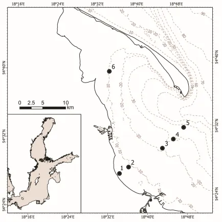
Sampling stations were located at a depth gradient in the central part of the bay (stations 1-5);
75
77
Figure 1. Study area and location of the sampling stations in the Gulf of Gdańsk (southern
78
Baltic Sea).
79
Conducted research included: investigation of spatial and temporal variations of hydrological
80
conditions (temperature and salinity) as well as investigations of the qualitative and quantitative
81
structure of three main copepod taxa (Acartia spp., Temora longicornis and Pseudocalanus acuspes).
82
Sampling was conducted during three separate projects spanning almost 14 years, from 1998 to 2012.
83
the first sampling period lasted from August 1998 to September 2000, the second took place in
84
2006-2007, and the last one in 2010-2012. During the sampling campaigns zooplankton samples were
85
collected with almost monthly coverage. Two types of sampling nets were used: from 1998 to 2007
86
samples were collected with a Copenhagen type net, and since 2010 the WP-2 type net was utilized.
87
Both types of nets were of 100 µm mesh size. Samples were collected with vertical hauls; at stations
88
shallower (1, 2, 6) haul was conducted from the bottom to the surface, while at deeper stations (3, 4,
89
5) the water column was divided into 10 m layers. All samples were collected during the daytime
90
(mainly between 11 am and 2 pm) so the diurnal vertical migrations were not accounted for. Along
91
with the collection of biological material water, physicochemical conditions (T, S) were measured.
92
2.3. Model data
94
The source of the numerical results used in the manuscript is the “Baltic Sea Biogeochemical
95
Reanalysis” product which provides a 24 years biogeochemical reanalysis for the Baltic Sea
96
(1993-2016) using the ice-ocean model NEMO-Nordic (based on NEMO-3.6, Nucleus for European
97
Modelling of the Ocean) coupled with the biogeochemical model SCOBI (Swedish Coastal and
98
Ocean Biogeochemical model) together with LSEIK data assimilation. Values for all the presented
99
variables (dissolved oxygen and chlorophyll a) have been derived from the daily means. Direct files
100
have been accessed and downloaded upon registration via a Copernicus Marine Environment
101
Monitoring Service’s (CMEMS) and choosing the BALTICSEA_REANALYSIS_BIO_003_012
102
product. Detailed description of the product is available as an online resource in the documentation
103
section. In particular, a Product User Manual [23] that covers detailed Production Subsystem
104
Description as well as Quality Report of the product [24] which provides an estimated accuracy
105
numbers for each variable summarized in the table below (Table 1).
106
Table 1. Estimated accuracy of the numerical model data according to quality information
107
document.
108
RMS error 0-5 m 5-30 m 30-80 m
Dissolved oxygen (mmol m-3 ) 19 38 51
Chlorophyll a (mg m-3) 5 3 0.9
109
Each in-situ station has been paired with the closest grid cell in the product’s model domain
110
estimating the minimal distance between station and each grid cell using longitude and latitude
111
meta information. Vertical means were calculated for the related timeseries.
112
2.4. Biomass and abundance
113
Collected zooplankton samples were analyzed in terms of qualitative and quantitative
114
descriptions of three copepod taxa, key for southern Baltic mesozooplankton populations: Acartia spp.
115
(including A.bifilosa, A.longiremis and A.tonsa), Temora longicornis and Pseudocalanus acuspes. All analysis
116
was performed in accordance with the HELCOM COMBINE methodology [25]. Obtained abundances
117
were then used to calculate the numbers of individuals per m2 and m3. Finally, standard weights [26]
118
were used to estimate the biomass values (mg C) of each of the taxa per m3.
119
Obtained biological data were normalized by transforming to natural logarithms (ln(x+1)).
120
Copepod abundances and biomasses were averaged over stations and the seasonal cycle was removed
121
subtracting long-term monthly means from annual monthly means.
122
Abundance values (ind. m-2) were next used to calculate secondary production rates and
123
mortality rates of the abovementioned copepod taxa.
124
2.5. Secondary production
125
Production rates of the investigated species were calculated with the Edmondson and Winberg
126
equation [27]. Calculations were carried out for each of the copepodite stages with assumption of
127
non-limiting food conditions:
128
PCi = Ni * ΔWi / Dmini, (1)
where PCi is daily potential production of stage i (wet weight), i is the development stage, Dmini is
129
the development time of stage i (day-1), ΔWi is the weight increase of stage i and Ni is the abundance
130
of stage i (ind. m-2). Dmin of developmental stages were computed using the function provided by
131
Figiela et al. [28]:
132
where Dmin is the minimum value of the development time, for which the growth rate of an
133
individual is not limited by food availability. The wet weights of the copepodite stages and adults
134
were accepted after Hernroth [26]. The conversion factor of 0.05 after Mullin [29] was used to
135
transform the wet weight to carbon content.
136
The development time D is a function of three variables: concentration of food Food (food
137
availability varying depending on season [22]), temperature T, and salinity S. Dmin was described for
138
each species at the nauplius and I to V copepodid developmental stages, by the equations described by
139
Figiela [28].
140
For Acartia spp.:
141
ft = {
1 for T <= 19 °C,
(3) 0.9957 e0.0181 (T – 19) for T >= 19 °C,
fs = 2 – (1 – exp (-0.9 (S – 0.001))), (4) Acartia spp. nauplii:
142
DN = [31.34 e-0.092 T + 4921.7 Food -1.7462 e-(0.1805 Food-0.1061) T] ft fs, (5)
Acartia spp. copepodite:
143
DC = [40.956 e-0.0849 T + 1178.5 Food -1.0486 e-(0.0739 Food0.1059) T] ft fs, (6)
For Temora longicornis:
144
ft = {
1 for T <= 15 °C,
(7) 0.9972 e0.0269 (T – 15) for T >= 15 °C,
fs = 2 – (1 – exp (-0.5 (S – 2))), (8)
Temora longicornis nauplii:
145
DN = [39.565 e-0.0964 T + 61 e -0.0081 Food e-(0.0006 Food + 0.0588) T] ft fs, (9)
Temora longicornis copepodite:
146
DC = [38.693 e-0.0809 T + 57.438 Food -0.0037 e-(0.0007 Food + 0.0517) T] ft fs, (10)
For Pseudocalanus acuspes:
147
ft = {
1 for T <= 14 °C,
(11) 0.9993 e0.0377 (T – 14) for T >= 14 °C,
fs = 3 – (2 – exp (-0.25 (S – 9))), (12)
Pseudocalanus acuspes nauplii:
148
DN = [41.342 e-0.069 T + 2.679 T1.0988 e(0.0209 ln T - 0.0829) Food] ft fs, (13)
Pseudocalanus acuspes copepodite:
149
DC = [34.888 e-0.0781 T + 1.786 e1.0988 ln T e(-0.0559 e-0.0486 T) Food] ft fs, (14)
Mortality rates of the three investigated taxa were computed with Aksnes and Ohman [1]
151
method, which is based on the abundances at different developmental stages.
152
While estimating mortality rate of stage i and i+1(θ) stage duration was considered for a period
153
equal to the corresponding duration of two consecutive stages (αi+αi+1) and it is assumed that the two
154
successive stages are taken impartially and are under the same influence of transport processes during
155
these stages. This led to the following formula of mortality estimates [1]:
156
For nauplii and copepodite stages CI to CIV:
157
(emDi – 1) / (1- e-mDi+1) = Zi / Zi + 1, (15)
For copepodite stage CV (since the stage duration of adults is infinite):
158
m = [ln (Zi / Zadult) +1] / Di, (16)
where Zi is the abundance of the developmental stage i, Zadultis the abundance of adults, Zi +1 is the
159
abundance of next stage (i +1), mi is instantaneous mortality rate of stage i (d-1), D followed by
160
subscripts are stage durations of copepodite stages i and i +1.
161
2.7. Statistical analyses
162
The obtained biomass of copepods developmental stages was square root transformed prior to
163
analysis. Similarities between samples were examined using the Euclidean distance index, depicted as
164
a non-metric multidimensional scaling (nMDS) [31], which illustrated similarities between analyzed
165
seasons. One-way Analyses of Similarities (ANOSIM) were performed in order to test the significance
166
between sampling seasons, years and stations. The association between temperature and each
167
developmental stage of all investigated copepod species was fitted using generalized linear models
168
(GLMs) with normal distribution. Additionally, means plots were carried out to illustrate the
169
production and mortality of different developmental stages of copepods according to analyzed
170
seasons. All analyses were performed in PRIMER version 7 [31] and CANOCO version 5 [32].
171
3. Results
172
3.1. Hydrology
173
The water temperature was characterized by a very similar distribution throughout the whole
174
study period, with summer to winter fluctuations typical for the temperate climate region. Mean
175
values of water temperature noted at the investigated region ranged from 0.57±0.43 °C in March
176
2006 to 18.42±3.03 °C in August 2010 (Figure 2).
177
Due to technical reasons, salinity values were not recorded during the first sampling campaign.
178
Recorded salinity fluctuations were minimal, and did not exceed 1; mean values ranged from
179
6.32±0.50 in July 2010 to 7.60±0.09 in March 2012 (Figure 2).
180
The mean oxygen concentration during the study was also relatively constant. The maximum
181
values were observed in the spring (about 400 mmol O2·m-3) and the minimum in August/September
182
(about 300 mmol O2·m-3) (Figure 2). The oxygen concentration was at the same level at all sampling
183
stations except stations shallower than 10 m (1, 2, 6), where it was generally slightly lower.
184
The highest mean values of chlorophyll a concentration was reached in May of 2010, 2011 and
185
2012 with average value about 9 mg m-3. In the spring/summer period the values were generally
186
over 5 mg m-3. The minimum chlorophyll a concentration was always noted in the winter. In the
187
annual cycle, usually two different peaks in chlorophyll a concentration was observed, in May and
188
September (Figure 2). The highest values of chlorophyll a concentration was noted at shallow
189
191
Figure 2. Water temperature, salinity, dissolved oxygen and chlorophyll a (± standard
192
deviation) in the Gulf of Gdańsk.
193
3.2. Abundance and biomass anomalies
194
Both abundance and biomass of the considered taxa were highly seasonal. After a decrease at
195
the beginning of the year, mainly in February, peak abundances and biomasses were found in
196
summer. In the case of Acartia spp. highest abundance was observed in August while biomass
197
peaked in July; for T.longicornis both abundance and biomass peaks were found in July; while
198
P.acuspes had it abundance peak in May, for biomass it was in August. The seasonal development,
199
with maximum abundance and biomass in summer, is confirmed by monthly long-term means
200
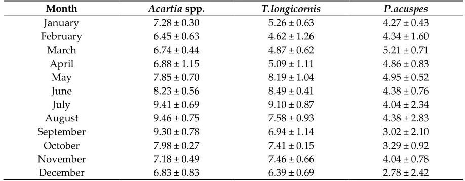
(Table 2, Table 3).
201
Table 2. Long-term monthly means (± standard deviation) for abundance (ln ind. m-3) of
202
three copepod taxa.
203
Month Acartia spp. T.longicornis P.acuspes
January 7.28 ± 0.30 5.26 ± 0.63 4.27 ± 0.43
February 6.45 ± 0.63 4.62 ± 1.26 4.34 ± 1.60
March 6.74 ± 0.44 4.87 ± 0.62 5.21 ± 0.71
April 6.88 ± 1.15 5.09 ± 1.11 4.86 ± 0.83
May 7.85 ± 0.70 8.19 ± 1.04 4.95 ± 0.52
June 8.23 ± 0.56 8.49 ± 0.41 4.38 ± 0.76
July 9.41 ± 0.69 9.10 ± 0.87 4.04 ± 2.34
August 9.46 ± 0.75 7.58 ± 0.93 4.38 ± 2.83
September 9.30 ± 0.78 6.94 ± 1.14 3.02 ± 2.10
October 7.98 ± 0.27 7.41 ± 0.15 3.29 ± 0.92
November 7.18 ± 0.49 7.46 ± 0.66 4.04 ± 0.78
December 6.83 ± 0.83 6.39 ± 0.69 2.78 ± 2.42
Table 3. Long-term monthly means (± standard deviation) for biomass (ln mgC m-3) of
204
Month Acartia spp. T.longicornis P.acuspes
January 2.08 ± 0.21 1.54 ± 0.48 0.69 ± 0.24
February 1.39 ± 0.74 1.29 ± 0.98 1.01 ± 1.17
March 1.62 ± 0.47 1.26 ± 0.44 1.01 ± 0.52
April 1.67 ± 0.80 1.13 ± 0.53 0.67 ± 0.33
May 2.55 ± 0.68 2.94 ± 0.69 0.41 ± 0.20
June 2.79 ± 0.59 3.21 ± 0.38 0.29 ± 0.12
July 4.08 ± 0.64 3.85 ± 0.77 0.62 ± 0.85
August 3.91 ± 0.56 3.01 ± 1.13 1.07 ± 0.80
September 3.83 ± 0.80 1.92 ± 0.80 0.40 ± 0.49
October 2.69 ± 0.27 2.45 ± 0.21 0.25 ± 0.21
November 1.87 ± 0.40 2.50 ± 0.58 0.47 ± 0.30
December 1.40 ± 0.53 1.52 ± 0.53 0.30 ± 0.28
The abundance and biomass of Acartia spp. (Figure 3) showed negative non-seasonal anomalies
206
during the first research period (1998-2000); it became positive during the second research period
207
(2007) and at the beginning of the third period (2010) to later become mostly negative (2011-2012).
208
The second of the investigated copepods, T.longicornis, also showed negative non-seasonal
209
anomalies during the period from 1998 to 2000, while in the second research period (2006-2007)
210
observed anomalies were mostly positive. This was also true for the beginning of 2010; later it came
211
closer to 0, and again positive at the end of 2011 (Figure 4). Anomalies for P.acuspes showed a similar
212
trend, with negative anomaly during the first research period, especially during 1998 and 1999.
213
During the second research period observed anomalies for that species were mostly positive, with a
214
drop at the end of 2007. In the third research period anomalies were mostly positive, especially in
215
2010, with occasional negative values in 2011 and 2012 (Figure 5).
216
217
219
Figure 4. Interannual (a) abundance and (b) biomass monthly mean and anomaly of Temora
220
longicornis.
221
222
Figure 5. Interannual (a) abundance and (b) biomass monthly mean and anomaly of Pseudocalanus
223
acuspes.
3.3. Secondary production
225
Considering the entire research period, inter-annual and seasonal variability of secondary
226
production of Acartia spp., T.longocornis and P.acuspes was visible. Obtained results showed that the
227
highest average secondary production was recorded during 2006 and 2007, while the lowest values
228
were observed from 1998 to 2000. During each of the years, the summer season was characterized by
229
the highest values of production rates (Figure 6).
230
231
Figure 6. Mean secondary production rates (± standard deviation) of for (a) Acartia spp., (b) Temora
232
longicornis and (c) Pseudocalanus acuspes in the Gulf of Gdańsk during particular seasons.
233
During the first research period, the average production rate for Acartia spp. reached the
234
highest value in the summer of 2000, almost 4 mg C m-2. In the second study period (2006-2007),
235
there was a large variation in the production rate. In summer 2007 it was more than 4 times higher
236
(about 16 mg C m-2) than recorded in the previous year. In the last years of research, a downward
237
tendency in production was observed, from about 8 mg C m-2 in the summer of 2010, to about 6 mg C
238
m-2 the following year, and finally about 4 mg C m-2 in summer 2012 (Figure 6).
239
The secondary production of T.longicornis was lower than for Acartia spp.. In the first years of
240
the study, from 1998 to 2000, the average maximum value in the summer fluctuated around 1 mg C
241
m-2. During the second time interval, similarly to Acartia spp., significant variations in production
242
values were observed, reaching around 2 mg C m-2 in summer 2006, and around 6 mg C m-2 a year
243
later. In following years of research, the highest average production rates were observed in
244
spring-summer periods. In 2010 it fluctuated between 2 mg C m-2 in spring to 1.8 mg C m-2 in
245
summer, while in 2011 and 2012, noted values were 1.7 mg C m-2 in spring and 2 mg C m-2 in
246
summer [Figure 6].
247
Among the investigated copepods, P.acuspes was characterized by the lowest secondary
248
production values. In the 1998-2000 period the average values of production rates of the species did
249
not exceed 25 µg C m-2 (summer 2000). During the second period of our research, two production
250
peaks were observed during each year. In 2006 the first was recorded in the summer with an average
251
value of around 175 µg C m-2, and the second one in the autumn – around 80 µg C m-2. In 2007 these
252
values were similar: in the summer the average production was 150 µg C m-2 and in autumn it
253
reached approximately 50 µg C m-2. During the last research period even lower production rate
254
values were observed. In 2010 and 2012 the average values did not exceed 50 µg C m-2, and the
255
maximum was observed in the summer of 2011, reaching 70 µg C m-2 (Figure 6).
256
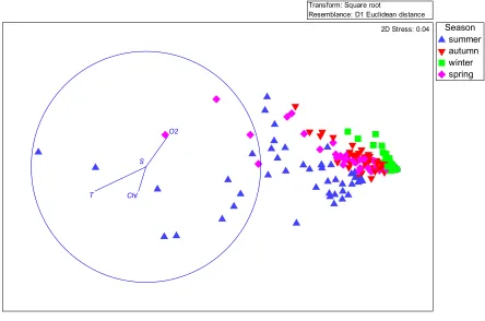
Obtained production values show significant differences between each designated season
257
on the nMDS plot (Figure 7). There is, however, a visible connection between spring and autumn
259
groups, which overlap partially (p=0.001, global R=0.089). The largest differences in production rates
260
were recorded between summer and winter (p=0.01, global R= 0.841).
261
Transform: Square root
Resemblance: D1 Euclidean distance
Season summer autumn winter spring
T
S
Chl
O2
2D Stress: 0.04
262
Figure 7. nMDS plot illustrating the samples ordination according to production rates based on the
263
seasons factor.
264
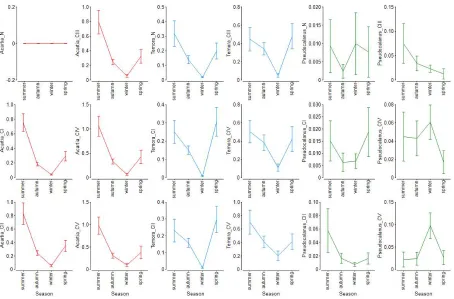
Generally, production rates of Acartia spp. for all stages were the highest in summer season
265
(Figure 8). Also, the range of production rates was highest in case of this taxon. T.longicornis showed
266
a similar trend, but during spring, production values were even higher than in summer, especially
267
for the youngest copepodites (CI-CIII). What is more, T.longicornis production values were generally
268
lower than for Acartia spp. (Figure 8). There was no visible tendency for production distribution of
269
P.acuspes stages. Nauplii production was the lowest in autumn, but during all seasons there were
270
very high discrepancies in production ranges. Copepodites CII and CIII production values were the
271
highest during the summer season, while the production rates of older CIV and CV increased in
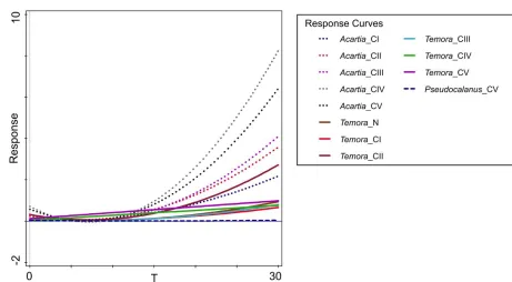
272
274
Figure 8. Means plot illustrating production distribution of Acartia spp., Temora longicornis and
275
Pseudocalanus acuspes developmental stages in relation to seasons.
276
GLM analysis revealed that, with increasing temperature, the production of Acartia spp. and
277
T.longicornis developmental stages increased, while stage CV of P.acuspes indicated almost neutral
278
correlation with temperature. The most intensive production rise with increasing temperature
279
demonstrated Acartia spp. stages (Table 4, Figure 9).
280
Table 4. Response of copepods developmental stages production to temperature (GLM
281
model).
282
Predictors T
Distribution normal
Link function identity
GLM fitted for 12 response variables:
Developmental stages Type R2[%] F p
Acartia spp._CI quadratic 18.4 18.4 <0.00001 Acartia spp._CII quadratic 1.0 17.4 <0.00001 Acartia spp._CIII quadratic 20.5 21.0 <0.00001 Acartia spp._CIV quadratic 24.6 26.6 <0.00001 Acartia spp._CV quadratic 20.9 21.5 <0.00001 Temora longicornis_N quadratic 19.5 19.8 <0.00001 Temora longicornis_CI quadratic 12.2 11.3 0.00002 Temora longicornis_CII quadratic 15.0 14.3 <0.00001 Temora longicornis_CIII quadratic 14.0 13.3 <0.00001
Temora longicornis_CIV linear 5.5 9.6 0.00229
Temora longicornis_CV linear 4.3 7.4 0.00732
283
284
Figure 9. Relationship of Acartia spp., Temora longicornis and Pseudocalanus acuspes
285
developmental stages with temperature from the generalized linear models (GLM).
286
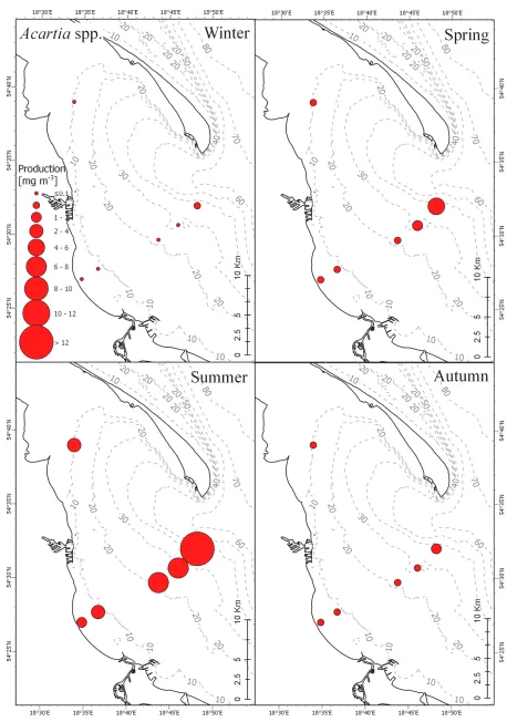
Horizontal distribution showed that the lowest average production rates of the three species in
287
the Gulf of Gdańsk were recorded at the shallow stations (1, 2, 6), while the deeper stations, mainly 4
288
and 5, were characterized by the highest production. The difference between production values
289
between the stations was particularly visible in the spring and summer seasons. Horizontal
290
distribution of secondary production of Acartia spp. showed the highest values for all six stations in
291
the summer (Figure 10). In the case of T.longicornis the highest production was observed in spring at
292
station 5, while in the summer the maximum production was recorded at station 4 (Figure 11). For
293
P.acuspes the highest production was noted in summer at station 5, while the lowest values were
294
296
297
Figure 10. Horizontal distribution of average secondary production rates of Acartia spp. in the Gulf
298
300
Figure 11. Horizontal distribution of average secondary production rates of Temora longicornis in the
301
303
Figure 12. Horizontal distribution of average secondary production rates of Pseudocalanus acuspes in
304
the Gulf of Gdańsk.
305
Mortality rates of the investigated species were diverse thorough the research period. The result
307
obtained for Acartia spp. showed the highest mortality rates mainly in summer, although in the
308
initial years of research a different trend was observed. In 1998 the highest mortality rate was
309
recorded in autumn (0.4 day-1), while in 2000 and 2006 the peak mortality rate was recorded in
310
spring. The highest rate of mortality of Acartia spp. was obtained in summer 2010, with a value of 0.8
311
day-1. Winter was characterized by lowest mortality, remaining during all years of research at a
312
similar level: about 0.2 day-1. Increased mortality rates of T.longicornis were usually noted for two
313
seasons, in summer-autumn 1999, spring-summer 2007, and spring-summer 2010-2012. These values
314
fluctuated between 0.5 day-1 to 0.7 day-1. However, the highest mortality rate of T.longicornis was
315
observed in spring 2006, reaching over 0.8 day-1. In winter mortality remained low, not exceeding 0.2
316
day-1. The mortality rates of P.acuspes showed a very irregular distribution throughout the study
317
period. In 1999 and 2007, two peaks were recorded, in winter and in summer. During 2006 and 2010
318
increased mortality of this species was observed during the summer season. Mortality rates in 2011
319
and 2012 remained at a similar level in all seasons (Figure 13).
320
321
Figure 13. Mean daily mortality rates (± standard deviation) for (a) Acartia spp., (b) Temora longicornis
322
and (c) Pseudocalanus acuspes in the Gulf of Gdańsk during seasons of investigation.
323
In context of mortality of individual development stages for Acartia spp. (N-CV) the highest
324
mortality was noted in the spring-summer period, and it concerned mainly the fifth copepodite
325
stage (CV). Maximum values were noted in spring 2006 and 2010, about 0.3 day-1, while in spring
326
2000 a high mortality rate was noted for CIII. In the second research period there was an increase in
327
mortality of nauplii, persisting from summer 2006 to winter 2007 (oscillating around 0.1 day-1), in
328
summer 2007 a high mortality rate of CIV (0.24 day-1) was also observed. The third time interval was
329
characterized by high mortality mainly among nauplii – about 0.2 day-1 and CV mortality, between
330
spring and autumn 2011 and 2012 (Figure 14a).
331
Considering mortality rates of T.longicornis stages during the first study period, the highest
332
values were observed for CIII, CIV and CV, ranging from 0.15 day-1 to 0.28 day-1. The lowest
333
mortality rate during that period was recorded for nauplii. In 2006-2007 and 2010-2012, the highest
334
mortality was observed for stages CII, CIII, CIV in spring and for nauplii in the summer, while for
335
CV two mortality peaks were noted, the first in spring and the second one in the autumn (Figure
336
14b).
337
For P.acuspes chaotic distribution of mortality of all stages was noted, which may have been
338
caused by a relatively low abundance of that species. High mortality rates for CIII in winter of 2010
339
341
Figure 14. Daily mortality rates of Copepoda stages N-CV for Acartia spp., Temora longicornis and
342
Pseudocalanus acuspes in the Gulf of Gdańsk during seasons of investigation.
343
When considering mortality rates in relation to seasons, significant differences were observed
344
(p=0.001, global R=0.355). The most visible differences in mortality rates were noted between winter
345
and spring seasons (p=0.001, global R=0.584) as well as between autumn and winter (p=0.001, global
346
R=0.539) (Figure 15).
347
Transform: Square root
Resemblance: D1 Euclidean distance
Season summer autumn winter spring
T S
2D Stress: 0.22
348
Figure 15. nMDS plot illustrating the samples ordination according to mortality rates based on the
349
seasons factor.
350
Mortality of Acartia spp. and T.longicornis was the lowest in autumn and winter for almost
351
all stages, with the exception of nauplii of both species, which achieved the lowest values of
352
was unspecified. However, nauplii demonstrated the highest mortality in summer and winter,
354
but CI and CII in spring. CIII and CIV in turn indicated the highest mortality in summer.
355
P.acuspes CV presented almost equal mortality for all seasons, but during autumn, the range of
356
values was the widest (Figure 16).
357
358
Figure 16. Means plot illustrating mortality distribution of Acartia spp., Temora longicornis and
359
Pseudocalanus acuspes developmental stages in relation to seasons.
360
Considering mortality rates, GLM plots showed positive, linear relationship between
361
T.longicornis stages (from N to CIV), Acartia spp. (CI, CII, CIV) and temperature. Both Acartia spp.
362
CV and T.longicornis CV demonstrated unimodal response along the temperature gradient, while
363
P.acuspes CV showed a negative relationship with temperature factor (Table 5, Figure 17).
364
Table 5. Response of copepods developmental stages mortality to temperature (GLM model).
365
Predictors T
Distribution normal
Link function identity
GLM fitted for 11 response variables:
Developmental stages Type R2[%] F p
Acartia spp._CI linear 5.1 8.9 0.00331
Acartia spp._CII linear 4.1 7.1 0.00868
Acartia spp._CIV linear 11.5 21.3 <0.00001
Acartia spp._CV quadratic 20.3 20.7 <0.00001
Temora longicornis_N linear 5.4 9.3 0.00266
Temora longicornis_CI linear 8.6 15.5 0.00012
Temora longicornis_CII linear 5.6 9.8 0.00206
Temora longicornis_CIV linear 4.0 6.9 0.00946
Temora longicornis_CV quadratic 8.6 7.7 0.00064
Pseudocalanus acuspes_CV linear 4.8 8.2 0.00478
366
367
Figure 17. Relationship of Acartia spp., Temora longicornis and Pseudocalanus acuspes developmental
368
stages with temperature from the generalized linear models (GLM).
369
Horizontal mortality distribution of Acartia spp. showed the highest mortality rate at the
370
shallow station 6 in spring and at stations 6, 1, 2 (> 0.68) in summer. In the autumn mortality rate of
371
Acartia spp. was within the same range at all stations (0.34 - 0.68). The lowest mortality was recorded
372
at station 6 in winter (0 - 0.17) (Figure 18).
373
The results for T.longicornis showed the highest mortality rates at stations 6 and 2 as well as at
374
station 3 in spring (> 0.64). In the summer season, at all stations the mortality rate was in the same
375
range (0.32 - 0.64). The lowest values were recorded in the winter at stations 6, 4 and 5 (0 - 0.08)
376
(Figure 19).
377
For P.acuspes, the horizontal mortality distribution showed the highest mortality at deep
378
stations 3 and 4 in the summer season (> 0.08). However, the lowest mortality was recorded at
379
381
382
384
Figure 19. Horizontal distribution of average mortality rates of Temora longicornis in the Gulf of
385
387
Figure 20. Horizontal distribution of average mortality rates of Pseudocalanus acuspes in the gulf of
388
Gdańsk.
389
4. Discussion
391
The aim of our study was a description of seasonal and interannual patterns of secondary
392
production and mortality rates for the main southern Baltic copepods. The main factors determining
393
zooplankton production are temperature and food availability [33]. Therefore we decided to
394
investigate seasonal and interannual fluctuations of secondary production of three copepod taxa:
395
Acartia spp., T.longicornis and P.acuspes in the southern Baltic. This is even more important in context
396
of increasing water temperatures observed in the Baltic related to global warming [34]. Higher water
397
temperature leads to shorter generation time and smaller body size of copepods, also causing
398
individuals to reach reproductive age quicker, and causing rapid increases in density [35]. However,
399
different copepod species have their individual temperature optimums, at which their development
400
is most optimal [21]. Therefore, when estimating the rate of secondary production of these copepods,
401
we used the Di function that takes into account the individual temperature optimums. We are also
402
aware that accurate estimates, most approximate to the natural state, of the secondary production
403
based on mathematical expressions require a method that combines a variety of factors. Because of
404
that our estimations do not fully reflect actual, real as in the natural environment, secondary
405
production values. However, they allow for an approximation of these values and enable
406
recognition of trends or anomalies occurring in the studied ecosystem.
407
Results obtained in our research showed clear correlation between seasonal production
408
fluctuations in the Gulf of Gdańsk and the hydrological conditions, mainly water temperature
409
(Figure 21). The highest correlation was recorded during summer, mainly for the young copepodite
410
stages of Acartia spp. as well as nauplii and copepodites of T.longicornis. This is consistent with
411
research carried out by Koski et al. [36] in the North Sea, which also indicates that the production
412
coefficient is significantly positively correlated with the average water temperature. However,
413
research from the Western Scheldt Estuary [37], showed that neither the biomass nor the secondary
414
copepod production was associated with chlorophyll concentration, and the temperature seemed to
415
have a significant impact only on the predominance of certain copepods. In contrary to those two
416
taxa, P.acuspes showed mostly negative correlation of secondary production with temperature. This
417
species in the central Baltic is associated with the deeper, more saline and also colder water layer
418
[38-40]. This was visible in high mean values of secondary production of nauplii and older
419
copepodites (CIV, CV) noted during winter seasons (Figure 8). We can therefore clearly state that,
420
similarly to other water basins, water temperature is one of the main factors controlling not only
421
biomass and abundance [17, 41] but also secondary production of main copepod taxa in the Gulf of
422
Gdańsk. Temperature was responsible for 11.8% of variability observed in RDA. In addition to
423
temperature, variability of secondary production was also to some extent explained by the
424
concentration of dissolved oxygen (5%) and chlorophyll a (4.5%) (Table 6).
425
Table 6. Explained variability and p values of particular environmental variables for redundancy
426
analysis (RDA).
427
Name Explains % pseudo-F p
Temperature (T) 11.8 15.6 0.001
Dissolved oxygen (O2) 5.0 7.0 0.002
Chlorophyll a 4.5 6.6 0.005
Salinity (S) 0.5 0.8 0.442
429
Figure 21. Ordination plot from redundancy analysis (RDA) on secondary production of
430
development stages of Acartia spp., Temora longicornis and Pseudocalanus acuspes (N – nauplii, CI-CV
431
copepodids of respective stage) and their relation to chlorophyll a and dissolved oxygen.
432
Comparison of the estimated values of secondary production of crustaceans from other regions
433
shows that that copepod production in the Gulf of Gdańsk is relatively low. The maximum
434
estimated average value of P.acuspes was (from the table) in the summer of 2007, while Renz [42]
435
described it as 26.2 mg C m-2 day-1 in June. Such a large difference in the obtained values is probably
436
due to differences in hydrological factors leading to differences in metabolic rates [40]. Renz and
437
Hirche [40] have shown that the rate of North Sea P.elongatus population development is about 3-5
438
times higher and the growth rate is up to 10 times higher than the P.acuspes population from the
439
Baltic Sea, which translates directly into the higher production of P.elongatus. Results reported by
440
Fransz [43] from the North Sea show that the secondary production of T.longicornis and Acartia clausi
441
fluctuated between 22-16 mgC m-2 between May and September. In the brackish waters of the
442
Western Scheldt Estuary, estimated maximum average secondary production of Acartia tonsa
443
oscillated around 25 mgC m-3 in August and the second peak was recorded in September with the
444
value of 8 mgC m-3. The presence of maxima of secondary production in these months is consistent
445
with the seasonality of production observed for these species from genus Acartia in the Gulf of
446
Gdańsk. Production values, as in the case of P.acuspes, were, however, lower than those recorded in
447
different calculation methods and wet mass converters for the copepod from various sources of
449
literature.
450
In the perspective of the observed progressing warming of the Baltic Sea, which is particularly
451
noticeable in its northern region (the air temperature in the spring increased by about 1.5 °C in the
452
period 1871-2011 [44]. The ecosystem of the southern Baltic – much more productive and biodiverse
453
– is more susceptible to the negative effects of such changes. Due to the currently observed
454
restructuring of unicellular plankton and the shift of phenological phases [45]. Further
455
comprehensive research on biological production in ecosystems is needed, combining the research
456
on primary phytoplankton production and the production of zooplankton. Observed progressing
457
delaying of the maximum of secondary production in relation to spring bloom of phytoplankton
458
may lead to serious consequences for the whole organic production and higher trophic levels in the
459
ecosystem [46].
460
Zooplankton mortality estimates are still not a well-developed parameter in determining
461
population dynamics. Therefore, selecting a proper methodology to describe this phenomenon can
462
be challenging, and the main uncertainty results from inherent difficulties in measuring this process
463
in the natural environment [47].
464
It is widely accepted that the daily copepod mortality decreases with consecutive
465
developmental stages or with an increase in size [48, 49]. Based on these assumptions we wanted to
466
describe mortality rates of main copepod taxa from the Gulf of Gdańsk at particular seasons of the
467
year. The results obtained for Acartia spp. and T.longicornis, however, show differences in mortality
468
for particular stages from that described by the above-mentioned authors. The highest mortality rate
469
for Acartia spp. was observed for the oldest copepodites (CV) with maximum values noted in spring:
470
about 0.3 day-1. For T.longicornis high rates were observed for CIII, CIV and CV, within a range from
471
0.15 day-1 to 0.28 day. High variability in mortality estimates between copepod species and
472
developmental stages in both spatial and seasonal distribution were also observed by other authors
473
[15, 50, 51].
474
In our research we observed cyclical changes in mortality, with the peak falling in the spring
475
and summer season. Maud et al. [52], on the other hand, recorded the highest mortality rates in
476
summer and autumn, with the lowest – as in our research – in winter. Differences in seasonality of
477
mortality in different regions may result from differences in the main cause of mortality. Mortality of
478
copepods can be caused by predatory (consumptive) or physicochemical and biological factors as
479
factors causing non-consumptive mortality. Consumptive mortality may be associated with the
480
abundance of predators [53] and is described in the literature as usually occurring in the autumn
481
season, when the abundance of predators is the highest. This type of mortality described for Calanus
482
helgolandicus constituted an average of 89% of the total mortality for this species [52]. In the Baltic
483
Sea, copepods are a valuable source of food for the commercially important fish species sprat and
484
herring, but jellyfish can also have a significant predatory impact. The gelatinous zooplankton was
485
the main cause of mortality variability observed in deep coastal sampling station located near
486
south-west of Plymouth, UK [54]. Non-consumer mortality may result from death caused by age
487
[55], diseases and parasitism [56], exposure to environmental pollution [57], and physiological stress
488
[58]. Field and laboratory studies show that non-consumptive factors can account for 25 to 33% of
489
the total death rate among adult copepods [59].
490
The species from genus Acartia had the highest abundance and biomass among the three
491
investigated taxa, while P.acuspes was far less abundant than the other two taxa. Such proportions
492
between those taxa is quite typical for the coastal region of the southern Baltic. P.acuspes tends to
493
dominate offshore areas of the Baltic Sea, is much less abundant in the coastal zones, and it is rarely
494
present above the thermocline, especially during the warm season [60, 61].
495
Observed long-term biomass means for Acartia spp. were in a similar range as those reported
496
for this region by Möllmann [34], while for T.longicornis and especially P.acuspes they were much
497
lower. This was probably due to our sampling stations being located mostly in the inner, coastal part
498
of the Gulf of Gdańsk. Möllmann [34] also showed mostly negative anomalies for both T.longicornis
499
consistent with our findings, which also showed strong positive anomalies for those taxa during the
501
first decade of the 2000s.
502
Author Contributions: Conceptualization, Lidia Dzierzbicka-Głowacka and Maja Musialik-Koszarowska;
503
Funding acquisition, Lidia Dzierzbicka-Głowacka; Investigation, Maja Musialik-Koszarowska, Marcin Kalarus
504
and Anna Lemieszek; Methodology, Maja Musialik-Koszarowska, Anna Lemieszek, Paula Prątnicka and Maciej
505
Janecki; Project administration, Lidia Dzierzbicka-Głowacka; Supervision, Maria Iwona Żmijewska;
506
Visualization, Marcin Kalarus and Paula Prątnicka; Writing – original draft, Maja Musialik-Koszarowska,
507
Marcin Kalarus, Anna Lemieszek, Paula Prątnicka and Maciej Janecki; Writing – review & editing, Lidia
508
Dzierzbicka-Głowacka.
509
Funding: Partial support for this study was provided by the project ‘Integrated info-prediction Web Service
510
WaterPUCK’ – no. BIOSTRATEG3/343927/3/NCBR/2017.
511
Acknowledgments: This study has been conducted using E.U. Copernicus Marine Service Information.
512
Calculations were carried out at the Academic Computer Centre in Gdańsk.
513
Conflicts of Interest: The authors declare no conflict of interest.
514
References:
515
1. Aksnes, D.L.; Ohman, M.D. A vertical life table approach to zooplankton mortality estimation. Limnol.
516
Oceanogr. 1996, 41, 7, 1461-1469.
517
2. Ohman, M.D.; Wood, S.N. Mortality estimation for planktonic copepods: Pseudocalanus newmani in a
518
temperate fjord. Limnol. Oceanogr. 1996, 41, 1, 126-135, doi:10.4319/lo.1996.41.1.0126.
519
3. Dzierzbicka-Głowacka, L.; Kalarus, M.; Musialik-Koszarowska, M.; Lemieszek, A.; Żmijewska, M.I.
520
Seasonal variability in the population dynamics of the main mesozooplankton species in the Gulf of
521
Gdańsk (southern Baltic Sea): Production and mortality rates. Oceanologia 2015, 57, 1, 78-85,
522
doi:10.1016/j.oceano.2014.06.001.
523
4. Corkett, C.J.; Zillioux, F.J. Studies on the effects of temperature on the egg laying of three species of
524
calanoid copepods in the laboratory (Acartia tonsa, Temora longicornis and Pseudocalanus elongatus). Bulletin
525
of the Plankton Society of Japan 1975, 21, 77-85.
526
5. Paffenhöfer, G.A.; Harris, R.P. Feeding, growth, and reproduction of the marine planktonic copepod
527
Pseudocalanus elongatus Boeck. J. Mar. Biol. Assoc. U. K. 1976, 56, 2, 327-344.
528
6. Klein Breteler, W.C.M.; Fransz, H.G.; Gonzalez, S.R. Growth and development of four calanoid copepod
529
species under experimental and natural conditions. Neth. J. Sea Res. 1982, 16, 195-207,
530
doi:10.1016/0077-7579(82)90030-8.
531
7. Koski, M.; Klein Breteler, W.C.M.; Schogt, N. Effect of food quality on rate of growth and development of
532
the pelagic copepod Pseudocalanus elongatus (Copepoda, Calanoida). Mar. Ecol. Prog. Ser. 1998, 170, 169-187,
533
doi:10.3354/meps119099.
534
8. Koski, M.; Klein Breteler, W.C.M. Influence of diet on copepod survival in the laboratory. Mar. Ecol. Prog.
535
Ser. 2003, 264, 73-82, doi:10.3354/meps264073.
536
9. Klein Breteler, W. C. M.; Schogt, N.; Rampen, S. Effect of diatom nutrient limitation on copepod
537
development: role of essential lipids. Mar. Ecol. Prog. Ser. 2005, 291, 125-133, doi:10.3354/meps291125.
538
10. Dzierzbicka-Głowacka, L.; Lemieszek, A.; Żmijewska, M.I. Development and growth of Temora longicornis:
539
numerical simulations using laboratory culture data. Oceanologia 2011, 53, 1, 137-161,
540
doi:10.5697/oc.53-1.137.
541
11. Kiørbe, T.; Johansen, K. Studies of a larval herring (Clupea harengus L.) patch in the Buchan area. IV.
542
Zooplankton distribution and productivity in relation to hydrographic features. Dana 1986, 6, 37-51.
543
12. Nielsen, T.G. Contribution of zooplankton grazing to the decline of a Ceratium bloom. Limnol. Oceanogr.
544
1991, 36, 6, 1091-1106.
545
13. Kiørbe, T.; Nielsen, T.G. Regulation of zooplankton biomass and production in a temperate, coastal
546
ecosystem. 1. Copepods. Limnol. Oceanogr. 1994, 39, 3, 493-507, doi:/10.4319/lo.1994.39.3.0493.
547
14. Halsband, C.; Hirche, H.J. Reproductive cycles of dominant calanoid copepods in the North Sea. Mar. Ecol.
548
Prog. Ser. 2001, 209, 219-229, doi:10013/epic.14539.d001.
549
15. Eiane, K.; Ohman, M.D. Stage specific mortality of Calanus finmarchicus, Pseudocalanus elongatus and
550
Oithona similis on Fladen Ground, North Sea, during a spring bloom. Mar. Ecol. Prog. Ser. 2004, 268,
551
16. Dzierzbicka-Głowacka, L.; Kalarus, M.; Żmijewska, M.I. Interannual variability in the population
553
dynamics of the main mesozooplankton species in the Gulf of Gdańsk (southern Baltic Sea): seasonal and
554
spatial distribution. Oceanologia 2013, 55, 2, 409-434, doi:10.5697/oc.55-2.409.
555
17. Musialik-Koszarowska, M.; Dzierzbicka-Głowacka, L.; Kalarus, M.; Lemieszek, A.; Maruszak, P.;
556
Żmijewska, M. I. Population dynamics of the main copepod species in the Gulf of Gdańsk (the southern
557
Baltic Sea): abundance, biomass and production rates. Oceanol. Hydrobiol. St. 2016, 45, 2, 159-171,
558
doi:10.1515/ohs-2016-0015.
559
18. Dzierzbicka-Głowacka, L. A numerical investigation of phytoplankton and Pseudocalanus elongatus
560
dynamics in the spring bloom time in the Gdańsk Gulf. J. Mar. Syst. 2005, 53, 1-4, 19-36.
561
19. Dzierzbicka-Głowacka, L.; Bielecka, L.; Mudrak, S. Seasonal dynamics of Pseudocalanus minutus elongatus
562
and Acartia spp. in the southern Baltic Sea (Gdańsk Deep) – numerical simulations. Biogeosciences 2006, 3,
563
635-650, doi:10.5194/bg-3-635-2006.
564
20. Dzierzbicka-Głowacka, L.; Żmijewska, M.I.; Mudrak, S.; Jakacki, J.; Lemieszek A. Population modelling of
565
Acartia spp. in a water column ecosystem model for the South-Eastern Baltic Sea. Biogeosciences 2010, 7,
566
2247-2259, doi:10.5194/bg-7-2247-2010.
567
21. Dzierzbicka-Głowacka, L.; Lemieszek, A.; Żmijewska, M.I. Development and growth of Temora longicornis:
568
numerical simulations using laboratory culture data. Oceanologia 2011, 53, 1, 137-161.
569
22. Dzierzbicka-Głowacka, L.; Kalarus, M.; Żmijewska, M.I. Interannual variability in the population
570
dynamics of the main mesozooplankton species in the Gulf of Gdańsk (southern Baltic Sea): seasonal and
571
spatial distribution. Oceanologia 2013, 55, 2, 409-434, doi:10.5697/oc.55-2.409.
572
23. Copernicus Marine Environment Monitoring Service’s (CMEMS).
573
http://marine.copernicus.eu/documents/QUID/CMEMSBAL- QUID-003-012.pdf (accessed on 23.03.2019).
574
24. Copernicus Marine Environment Monitoring Service’s (CMEMS).
575
http://marine.copernicus.eu/documents/QUID/CMEMS-BALQUID- 003-012.pdf (accessed on 23.03.2019).
576
25. HELCOM, 2017. Manual for Marine Monitoring in the COMBINE Programme of HELCOM.
577
http://helcom.fi/action-areas/monitoring-and-assessment/manuals-and-guidelines/combine-manual/(acce
578
ssed 20.02.2019).
579
26. Hernroth, L. Recommendations on methods for marine biological studies in the Baltic Sea:
580
Mesozooplankton Biomass Assessment. The Baltic Marine Biologists 1985, 10, 1-32.
581
27. Edmondson, W.T.; Winberg, G.G. A Manual on Methods for the Assesment of Secondary Productivity in
582
Freshwaters, 1971, IPB Handbook, 17, pp. 358.
583
28. Figiela, M.; Musialik-Koszarowska, M.; Nowicki, A.; Lemieszek, A.; Kalarus, M.; Druet, Cz. Long-term
584
changes in the total development time of Copepoda species occurring in large numbers in the Southern
585
Baltic Sea -numerical calculations. Oceanol. Hydrobiol. St. 2016, 45, 1, 1-10.
586
29. Mullin, M.M. Production of zooplankton in the ocean: the present status and problems. Oceanogr. Mar.
587
Biol. Rev. 1969, 7, 293-310.
588
30. Aksnes, D.L.; Ohman, M.D. A vertical life table approach to zooplankton mortality estimation. Limnol.
589
Oceanogr. 1996, 41,7, 1461–1469, doi:10.4319/lo.1996.41.7.1461.
590
31. Clarke, K.R.; Gorley, R.N. 2015. PRIMER v7: user manual/tutorial. PRIMER-E, Plymouth.
591
32. Ter Braak, C.J.F.; Šmilauer, P. Canoco reference manual and user's guide: software for ordination, version 5.0.
592
2012, USA, Ithaca: Microcomputer Power.
593
33. Richardson, A. J. In hot water: zooplankton and climate change. ICES J. Mar. Sci. 2008, 65, 279–295,
594
doi:10.1093/icesjms/fsn028.
595
34. Möllmann, C.; Kornilovs, G.; Sidrevics, L.; Long-term dynamics of main mesozooplankton species in the
596
central Baltic Sea. J. Plankton Res. 2000, 22, 11, 2015–2038, doi:10.1093/plankt/22.11.2015.
597
35. Gillooly, J. Effect of body size and temperature on generation time in zooplankton, J. Plankton Res. 2000, 22,
598
2, 241–251, doi:10.1134/S1995082909030079.
599
36. Koski, M.; Jonasdottir, S. H.; Bagøien, E. Biological processes in the North Sea II. Vertical distribution and
600
reproduction of neritic copepods in relation to environmental factors. J. Plankton Res. 2010, 51, 1, 63–84,
601
doi:10.1093/plankt/fbq084.
602
37. Escaravage, V.; Soetaert, K. Secondary production of the brackish copepod communities and their
603
contribution to the carbon fluxes in the Westershelde estuary (The Netherlands), Hydrobiologia 1995, 311, 1,
604
38. Frost, B.W. A taxonomy of the marine calanoid copepod genus Pseudocalanus. Can. J. Zool. 1989, 67,
606
525-551, doi:10.1139/z89-077.
607
39. Bucklin, A.; Frost, B.W.; Bradford-Grieve, J.; Allen, L.D.; Copley, N.J. Molecular systematic and
608
phylogenetic assessment of 34 calanoid copepod species of the Calanidae and Clausocalanidae. Mar. Biol.
609
2003, 142, 333-343, doi:10.1007/s00227-002-0943-1.
610
40. Renz, J.; Hirche, H.J. Life cycle of Pseudocalanus acuspes Giesbrecht (Copepoda, Calanoida) in the Central
611
Baltic Sea: I. Seasonal and spatial distribution. Mar. Biol. 2006, 148, 567–580, doi:10.1007/s00227-005-0103-5.
612
41. Musialik-Koszarowska, M.; Dzierzbicka-Głowacka, L.; Weydmann, A. Influence of environmental factors
613
on the population dynamics of key zooplankton species in the Gulf of Gdańsk (Southern Baltic Sea).
614
Oceanologia 2019, 177, 1-9, doi:10.1016/j.oceano.2018.06.001.
615
42. Renz, J.; Mengedoht, D.; Hirche, H.J. Reproduction, growth and secondary production of Pseudocalanus
616
elongatus Boeck (Copepoda, Calanoida) in the southern North Sea. J. Plankton Res. 2008, 30, 5, 511-528,
617
doi:10.1093/plankt/fbn016.
618
43. Fransz, H.G.; Miquel, J.C.; Gonzalez, S.R. Mesozooplankton composition, biomass and vertical
619
distribution, and copepod production in the stratified Central North Sea. Neth. J. Sea Res. 1984, 8, 82-96,
620
doi:10.1016/0077-7579(84)90026-7.
621
44. The BACC II, Author Team, 2008. Second Assessment of Climate Change for the Baltic Sea Basin. Regional
622
Climate Studies. 1–22 pp., Springer International Publishing, http://dx.doi.org/10.1007/978-3-319-16006-1
623
(accessed on 18.01.2019).
624
45. Allen, J.L.; Anderson, D.; Burford, M.; Dyhrman, S.; Flynn, K.; Gilbert, P.M.; Grane’li, E.; Heil, C.; Sellner,
625
K.; Smayda, T.; Zhou, M. Global ecology and oceanography of harmful algal blooms in eutrophic systems.
626
GEOMAP report 4, IOC and SCOR., Paris, France and Baltimore, 2006, MD, USA, 1-74 pp.
627
46. Fransz, H.G., Miquel, J.C. and Gonzalez, S.R. Mesozooplankton composition, biomass and vertical
628
distribution, and copepod production in the stratified Central North Sea. Neth. J. Sea Res. 1984, 18, 82-96
629
47. Ohman, M.D.; Wood, S.N. The inevitability of mortality. ICES J. Mar. Sci. 1995, 52, 517–522,
630
doi:10.1016/1054-3139(95)80065-4.
631
48. Cushing, D. H. The possible density-dependence of larval mortality and adult mortality in fishes. In J. H.
632
S. Blaxter [ed.], The early life history of fish. Springer-Verlag, New York, Heidelberg, Berlin, 1974, p.
633
103-111.
634
49. Peterson, I.; Wróblewski, S.J. Mortality rate of fishes in the pelagic ecosystem. Can. J. Fish. Aquat. Sci. 1984,
635
41, 1117-1120, doi:10.1139/f84-131.
636
50. Thor, P.; Nielsen, T.G.; Tiselius, P. Mortality rates of epipelagic copepods in the post-spring bloom period
637
in Disko Bay, western Greenland. Mar. Ecol. Prog. Ser. 2008, 359, 151–160, doi:10.3354/meps07376.
638
51. Plourde, S.; Pepin, P.; Head, E.J.H. Long-term seasonal and spatial patterns in mortality and survival of
639
Calanus finmarchicus across the Atlantic Zone Monitoring Programme region, northwest Atlantic. ICES J.
640
Mar. Sci. 2009b, 66: 1942–1958, doi:10.1093/icesjms/fsp167.
641
52. Maud, J. L.; Atkinson, A.; Hirst, A. G.; Lindeque, P. K.; Widdicombe, C. L.; Harmer, R. A.; McEvoy, A. J.;
642
Cummings, D. G. How does Calanus helgolandicus maintain its population in a variable environment?
643
Analysis of a 25-year time series from the English Channel. Prog. Oceanogr. 2015, 137, 513– 523,
644
doi:10.1002/lno.10805.
645
53. Ohman, M.D.; Durbin, E.G.; Runge, J.A.; Sullivan, B.K.; Field, D.B. Relationship of predation potential to
646
mortality of Calanus finmarchicus on Georges Bank, northwest Atlantic. Limnol. Oceanogr. 2008, 53,
647
1643–1655, doi:10.4319/lo.2008.53.4.1643.
648
54. Hernroth, L.; Grondahl, F. On the Biology of Aurelia aurita. Ophelia, 1993, 22, 2, 189-199,
649
doi:10.1080/00785326.1983.10426595.
650
55. Rodriguez-Grana, L.; Calliari, D.; Tiselius, P.; Hansen, B.W.; Skold, H.N. Gender-specific ageing and
651
non-Mendelian inheritance of oxidative damage in marine copepods. Mar. Ecol. Prog. Ser. 2010, 401, 1–13,
652
doi:10.3354/meps08459.
653
56. Kimmerer, W.J.; McKinnon, A.D. High mortality in a copepod population caused by a parasitic
654
dinoflagellate. Mar. Biol. 1990, 107, 449–452, doi:10.1007/BF01313428.
655
57. Wendt, I.; Backhaus, T.; Blanck, H.; Arrhenius, Å. The toxicity of the three antifouling biocides DCOIT,
656
TPBP and medetomidine to the marine pelagic copepod Acartia tonsa. Ecotoxicology 2016, 25, 871– 879,