Abstract--Histogram is a graphical representation showing a visual impression of the distribution of experimental data. It is an estimate of the probability distribution of a continuous variable and was first introduced by Karl Pearson. A histogram consists of tabular frequencies, shown as adjacent rectangles, erected over discrete intervals (bins), with an area equal to the frequency of the observations in the interval. In this paper the comparative analysis of various Image Edge Detection techniques for Power Amplifier is presented with histogramic implementation. The software is developed using MATLAB 7.5. Evaluation of the images showed that under noisy conditions Canny, LoG( Laplacian of Gaussian), Robert, Prewitt, Sobel exhibit better performance, respectively[1]. Histograms are used to get better results which helps to plot the number of pixels for each tonal value. By looking at the histogram for a specific image a viewer will be able to judge the object edge detection is one of the ways of solving the problem of high volume of space images occupy in the computer memory. The problems of storage, transmission over the Internet and bandwidth could be solved when edges are detected.
Keywords—Histogram, Histogram equalization, Edge detection techniques, Power Amplifier.
I.INTRODUCTION
Histograms are used to analyse the tonal value of an image. It shows how bright or dark the image is (number of tones captured at each brightness level) It is made of individual columns (each column representing how many pixels there are in specific tonal value) which range from darkest (value 0) to brightest (value 255).Between the two are the gray values. A Histogram reveals the inform-ation that whether or not your image has been properly scanned or exposed. Each pixel in an image has a color which has been produced by some combination of the primary colors red, green, and blue (RGB). Each of these colors can have a brightness value ranging from 0 to 255 for a digital image with a bit depth of 8-bits. A RGB histogram results when the computer scans through each of these RGB brightness values and counts how many are at each level from 0 through 255.Histograms are merely the representative of tonal value of an image. Image processing is a technique which involves enhancement or manipulation of an image which resulted in another image, removal of redund-ant data and the transformation of a 2-D and 3-D pixel array
into a statically uncorrelated data set. Images as a whole contains redundant data and important information lies in the edges of an image. Edges correspond to object boundaries, changes in surface orientation and describe defeat by a small margin. Thus, detecting Edges of power amplifier help in extracting useful information characteristics of the image where there are abrupt changes. The two filters highlight areas of high special frequency, which tend to define the edge of an object in an image. The two filters are designed with the intention of bringing out the diagonal edges within the image. The Gx image will enunciate diagonals that run from the top-left to the bottom-right where as the Gy image will bring out edges that run top right to bottom-left. The two individual images Gx andGy are combined using the approximation equation
G Gx Gy
II.HISTOGRAM EQUALIZATION
It is a method in image processing of contrast adjustment using the image's histogram. With this the intensities can be better distributed on the histogram. It has got applications in the field of thermal, satellite,or X-ray images. This technique is basically used to improve the visuality of an image.Basically in this technique for recovering some of apparently lost contrast in an image by remapping the brightness values in such a way as to equalize, or more evenly distribute, its brightness values. The method to draw the equalized histogram is given below:
1) Read the input image: The input image contains n pixcls where n=height*width.
2) Convert form RGB.
3) Calculate the Histogram: The Histogram og input image is calculated. This is a 256 value array, where H[x] contains the number of pixels with value x.
4) Calculation of C.D.F: The C.D.F of histogram is calculated. This is a 256 value array, where cdf[x] contains the number of pixels with value x or less:
cdf[x] = H[0] + H[1] + H[2] + ... + H[x] 5) Loop through the n pixels in the entire image and replace the value at each i'th point:
V[i] <-- floor(255*(cdf[V[i]] - cdf[0])/(n - cdf[0])) 6) Convert the image back from HSV to RGB.
7)Save the image in the desired format and file name.
Analysis of Power Amplifier by Frontier
Recognition and Histograms
Surekha Chauhan
*1, Prof. P.K. Ghosh
1,Madan Shishodia
21
ECE Deptt.,
Mody institute of Technology and Science, Rajasthan
INDIA
2
III. POWER AMPLIFIER
Generally, an amplifier is any device that changes, usually
increases, strength of a signal. Power amplifier is a type
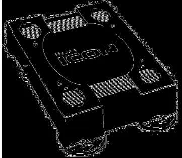
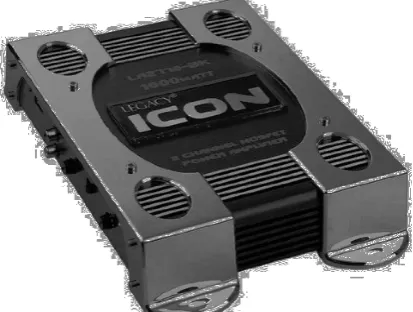
of electronic amplifier used to convert a low-power radio-frequency signal into a larger signal of significant power, typically for driving the antenna of a transmitter. It is usually optimized to have high efficiency, high output Power. Noise is an undesirable but inevitable product of the electronic devices specially in low level signals .So this technique of edge detection before designing will help to increase efficiency of power amplifier by reducing the noise in it.(fig. 1).
Fig1. Input gray Scale Power Amplifier
.
IV.EDGE DETECTION TECHNIQUES Sobel Operator
The operator consists of a pair of 3×3 convolution kernels as shown in Figure 1. One kernel is simply the other rotated by 90°.
-1 0 +1 -2 0 +2 -1 0 +1
Gx Gy
Fig. 2: Masks used by Sobel Operator
These kernels are designed to respond maximally to edges running vertically and horizontally relative to the pixel grid, one kernel for each of the two perpendicular orientations. The kernels can be applied separately to the input image, to produce separate measurements of the gradient component in each orientation (call these Gx and Gy). These can then be combined together to find the absolute magnitude of the gradient at each point and the orientation of that gradient[3]. The gradient magnitude is given by:
2 2
Gy
Gx
G
Typically, an approximate magnitude is computed using:
Gy
Gx
G
which is much faster to compute.
The angle of orientation of the edge (relative to the pixel grid) giving rise to the spatial gradient is given by:
)
/
arctan(
Gy
Gx
0 0.5 1 1.5 2 2.5
x 104
0 50 100 150 200 250
Fig.3: Histogram of Sobel Edge detection
Fig. 4: Edges retrieve by Sobel Operator
Robert’s cross operator
The Roberts Cross operator performs a simple, quick to compute, 2-D spatial gradient measurement on an image. Pixel values at each point in the output represent the estimated absolute magnitude of the spatial gradient of the input image at that point. The operator consists of a pair of 2×2 convolution kernels as shown in Figure 2. One kernel is simply the other rotated by 90°[4]. This is very similar to the Sobel operator.
Gx
Gy Fig.5: Masks used for Robert operator.
These kernels are designed to respond maximally to edges running at 45° to the pixel grid, one kernel for each of the two perpendicular orientations. The kernels can be applied separately to the input image, to produce separate measurements of the gradient component in each orientation (call these Gx and Gy). These can then be combined together +1 +2 +1
0 0 0 -1 -2 -1
+1 0
to find the absolute magnitude of the gradient at each point and the orientation of that gradient. The gradient magnitude is given by:
2 2
Gy
Gx
G
although typically, an approximate magnitude is computed using:
Gy
Gx
G
which is much faster to compute.
The angle of orientation of the edge giving rise to the spatial gradient (relative to the pixel grid orientation) is given by:
4
/
3
)
/
arctan(
Gy
Gx
Fig. 6: Edges retrieve by Robert Cross Operator
Prewitt’s operator
Prewitt operator [5] is similar to the Sobel operator and is used for detecting vertical and horizontal edges in images.
-1 0 +1 -1 0 +1 -1 0 +1
Gx Gy Fig 7: Masks for the Prewitt gradient edge detector
Fig. 8: Edges retrieve by Prewitt Operator
Laplacian of Gaussian
The Laplacian is a 2-D isotropic measure of the 2nd spatial derivative of an image. The Laplacian of an image highlights regions of rapid intensity change and is therefore often used for edge detection. The Laplacian is often applied to an image that has first been smoothed with something approximating a Gaussian Smoothing filter in order to reduce its sensitivity to noise. The operator normally takes a color image which converts to gray level image as input by software and produces another gray level image as output. The Laplacian L(x,y) of an image with pixel intensity values I(x,y) is given by:
L(x,y)=
2I +
2I
x2
y2Since the input image is represented as a set of discrete pixels, we have to find a discrete convolution kernel that can approximate the second derivatives in the definition of the Laplacian[5].
Fig. 9:Mask for Laplacian of Gaussian Detector
Because these kernels are approximating a second derivative measurement on the image, they are very sensitive to noise. To counter this, the image is often Gaussian Smoothed before applying the Laplacian filter. This pre-processing step reduces the high frequency noise components prior to the differentiation step. In fact, since the convolution operation is associative, we can convolve the Gaussian smoothing filter with the Laplacian filter first of all, and then convolve this hybrid filter with the image to achieve the required result. Doing things this way has two advantages: Since both the Gaussian and the Laplacian kernels are usually much smaller than the image, this method usually requires far fewer arithmetic operations. The LoG (`Laplacian of Gaussian')[6] kernel can be pre-calculated in advance so only one convolution needs to be performed at run-time on the image. The 2-D Laplacian of Gaussian (LoG) function. The x and y axes are marked in standard deviations (
).LoG(x,y)= -1/
4[ 1- (2 2 2
2
y
x
)] 2
2 2
2
y x
e
Note that as the Gaussian is made increasingly narrow, the LoG kernel becomes the same as the simple Laplacian kernels shown in figure 4. This is because smoothing with a very narrow Gaussian (
< 0.5 pixels) on a discrete grid has no effect. Hence on a discrete grid, the simple Laplacian can be seen as a limiting case of the LoG for narrow Gaussians [8]-[10].+1 +1 +1 0 0 0 -1 -1 -1
1 1 1 1 -8 1 1 1 1
0 1 0 1 -4 1 0 1 0 -1 2 -1
Fig. 10: Edges retrieve by Laplacian method
Canny Edge Detection Algorithm
The Canny edge detection algorithm is known to many as the optimal edge detector. His criteria is to improve current methods of edge detection. The first and most obvious is low error rate. It is important that edges occurring in images should not be missed and that there be no responses to non-edges. The second criterion is that the edge points be well localized. In other words, the distance between the edge pixels as found by the detector and the actual edge is to be at a minimum. A third criterion is to have only one response to a single edge. This was implemented because the first two were not substantial enough to completely eliminate the possibility of multiple responses to an edge. Based on these criteria, the canny edge detector first smoothes the image to eliminate and noise. It then finds the image gradient to highlight regions with high spatial derivatives.
Step 1:-In order to implement the canny edge detector
algorithm, a series of steps must be followed. The first step is to filter out any noise in the original image before trying to locate and detect any edges. And because the Gaussian filter can be computed using a simple mask, it is used exclusively in the Canny algorithm. Once a suitable mask has been calculated, the Gaussian smoothing can be performed using standard convolution methods. A convolution mask is usually much smaller than the actual image. As a result, the mask is slid over the image, manipulating a square of pixels at a time. The larger the width of the Gaussian mask, the lower is the detector's sensitivity to noise. The localization error in the detected edges also increases slightly as the Gaussian width is increased.
Step 2:- After smoothing the image and eliminating the noise,
the next step is to find the edge strength by taking the gradient of the image. The Sobel operator performs a 2-D spatial gradient measurement on an image. Then, the approximate absolute gradient magnitude (edge strength) at each point can be found. The Sobel operator [3] uses a pair of 3x3 convolution masks, one estimating the gradient in the x-direction (columns) and the other estimating the gradient in the y-direction (rows). They are shown below
:
-1 0 +1 -2 0 +2 -1 0 +1
Gx Gy
Fig. 11:Mask for Canny Edge Detector Technique The magnitude, or edge strength, of the gradient is then approximated using the formula:
|G| = |Gx| + |Gy|
Step 3:- The direction of the edge is computed using the
gradient in the x and y directions. However, an error will be generated when sumX is equal to zero. So in the code there has to be a restriction set whenever this takes place. Whenever the gradient in the x direction is equal to zero, the edge direction has to be equal to 90 degrees or 0 degrees, depending on what the value of the gradient in the y-direction is equal to. If GY has a value of zero, the edge direction will equal 0 degrees. Otherwise the edge direction will equal 90 degrees. The formula for finding the edge direction is just:
Theta = inv tan (Gy / Gx)
Step 4:- Once the edge direction is known, the next step is to
relate the edge direction to a direction that can be traced in an image. So if the pixels of a 5x5 image are aligned as follows: x x x x x
x x x x x x x a x x x x x x x x x x x x
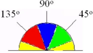
Then, it can be seen by looking at pixel "a", there are only four possible directions when describing the surrounding pixels - 0 degrees (in the horizontal direction), 45 degrees (along the positive diagonal), 90 degrees (in the vertical direction), or 135 degrees (along the negative diagonal). So now the edge orientation has to be resolved into one of these four directions depending on which direction it is closest to (e.g. if the orientation angle is found to be 3 degrees, make it zero degrees). Think of this as taking a semicircle and dividing it into 5 regions.
Fig.:12 Semicircle showing possible orientation of pixel.
Therefore, any edge direction falling within the yellow range (0 to 22.5 & 157.5 to 180 degrees) is set to 0 degrees. Any edge direction falling in the green range (22.5 to 67.5 degrees) is set to 45 degrees. Any edge direction falling in the blue range (67.5 to 112.5 degrees) is set to 90 degrees. And finally, any edge direction falling within the red range (112.5 to 157.5 degrees) is set to 135 degrees.
Step 5:- After the edge directions are known, non-maximum
suppression now has to be applied. Non-maximum suppression is used to trace along the edge in the edge direction and suppress any pixel value (sets it equal to 0) that is not considered to be an edge. This will give a thin line in the output image.
Step 6:- Finally, hysteresis [12] is used as a means of
eliminating streaking. Streaking is the breaking up of an edge contour caused by the operator output fluctuating above and below the threshold. If a single threshold, T1 is applied to an image, and an edge has an average strength equal to T1, then due to noise, there will be instances where the edge dips below the threshold. Equally it will also extend above the threshold making an edge look like a dashed line. To avoid this, hysteresis uses 2 thresholds, a high and a low
0 0.5 1 1.5 2 2.5
x 104
0 50 100 150 200 250
under noisy conditions. So edge Detection and histogram techniques are very important factor in image processing as it is used in variety of applications of machine vision and medical sciences. Various edge detection techniques if implemented by a histogram gives better results according to the need. It has been shown that the Canny’s edge detection algorithm performs better than all these operators. In our experiment also Canny Edge Detection Algorithm gives best results in removing redundancy and enhance efficiency. Addition of Histograms helps us to get the edges for JPEG images also. This paper gives good result by addition of histograms to edge detection techniques. This technique is also be used in almost wide fields of mosfet frontier diction, medical equipments machines, and many VLSI embedded devices also help retain efficiency of Power Amplifier by reducing its noise.
Fig. 13 Edges retrieve by Canny Operator
Fig.14 Histogram of Canny Edge detection
V. Conclusions
Histogram is a technique which helps us to evaluate the structural properties of an image well. It helps us to obtain better visual quality of an image because of which the edges detected by various techniques are prone to noise. Hence the efficiency of device increases and they perform well
REFERENCES
[I] E. Argyle. “Techniques for edge detection,” Proc. IEEE, vol. 59, pp. 285-286, 1971
[2] F. Bergholm. “Edge focusing,” in Proc. 8th Int. Conf. Pattern Recognition,Paris, France, pp. 597- 600, 1986 [3] J. Matthews. “An introduction to edge detection: The
sobel edge detector,” Available at http://www.generation5.org/content/2002/im01.asp,
2002.
[4] L. G. Roberts. “Machine perception of 3-D solids” ser. Optical and Electro-Optical Information Processing. MIT Press, 1965 .
[5] R. C. Gonzalez and R. E. Woods. “Digital Image Processing”. 2nd ed. Prentice Hall, 2002.
[6] V. Torre and T. A. Poggio. “On edge detection”. IEEE Trans. Pattern Anal. Machine Intell., vol. PAMI-8, no. 2, pp. 187-163, Mar. 1986.
[7] E. R. Davies. “Constraints on the design of template masks for edge detection”. Partern Recognition Lett., vol. 4, pp. 11 1-120, Apr. 1986.
[8] W. Frei and C.-C. Chen. “Fast boundary detection: A generalization and a new algorithm ”. lEEE Trans. Comput., vol. C-26, no. 10, pp. 988-998, 1977.