Probabilistic Modeling and Bayesian Inference of Metal-Loss Corrosion with Application in Reliability Analysis for Energy Pipelines

(1)

Scholarship@Western

Electronic Thesis and Dissertation Repository

8-27-2014 12:00 AM

Probabilistic Modeling and Bayesian Inference of Metal-Loss

Corrosion with Application in Reliability Analysis for Energy

Pipelines

Hao Qin

The University of Western Ontario

Supervisor Wenxing Zhou

The University of Western Ontario

Graduate Program in Civil and Environmental Engineering

A thesis submitted in partial fulfillment of the requirements for the degree in Master of Engineering Science

Follow this and additional works at: https://ir.lib.uwo.ca/etd

Part of the Civil Engineering Commons, and the Structural Engineering Commons

Recommended Citation Recommended Citation

Qin, Hao, "Probabilistic Modeling and Bayesian Inference of Metal-Loss Corrosion with Application in Reliability Analysis for Energy Pipelines" (2014). Electronic Thesis and Dissertation Repository. 2246. https://ir.lib.uwo.ca/etd/2246

This Dissertation/Thesis is brought to you for free and open access by Scholarship@Western. It has been accepted for inclusion in Electronic Thesis and Dissertation Repository by an authorized administrator of

(2)

ENERGY PIPELINES

(Thesis format: Integrated Article)

by

Hao Qin

Graduate Program in Engineering Science Department of Civil and Environmental Engineering

A thesis submitted in partial fulfillment of the requirements for the degree of

Master of Engineering Science

The School of Graduate and Postdoctoral Studies The University of Western Ontario

London, Ontario, Canada

(3)

ii

The stochastic process-based models are developed to characterize the generation

and growth of metal-loss corrosion defects on oil and gas steel pipelines. The generation

of corrosion defects over time is characterized by the non-homogenous Poisson process,

and the growth of depths of individual defects is modeled by the non-homogenous

gamma process (NHGP). The defect generation and growth models are formulated in a

hierarchical Bayesian framework, whereby the parameters of the models are evaluated

from the in-line inspection (ILI) data through the Bayesian updating by accounting for

the probability of detection (POD) and measurement errors associated with the ILI data.

The Markov chain Monte Carlo (MCMC) simulation in conjunction with the data

augmentation (DA) technique is employed to carry out the Bayesian updating.

Numerical examples that involve both the simulated and actual ILI data are used to

validate the proposed Bayesian formulation and illustrate the application of the

methodology.

A simple Monte Carlo simulation-based methodology is further developed to

evaluate the time-dependent system reliability of corroding pipelines in terms of three

distinctive failure modes, namely small leak, large leak and rupture, by incorporating the

corrosion models evaluated from the Bayesian updating methodology. An example that

involves three sets of ILI data for a pipe joint in a natural gas pipeline located in Alberta

is used to illustrate the proposed methodology. The results of the reliability analysis

indicate that ignoring generation of new defects in the reliability analysis leads to

underestimations of the probabilities of small leak, large leak and rupture. The

generation of new defects has the largest impact on the probability of small leak.

Keywords

Pipeline; Metal-loss corrosion; Stochastic process; Hierarchical Bayesian; Measurement

error; Probability of detection; Missing data; Markov chain Monte Carlo; Data

(4)

iii

(5)

iv

First of all, I would express all my gratitude and appreciation to my supervisor Dr.

Wenxing Zhou, for his continuous support and patient guidance throughout this study.

His expertise and academic attitude always help and encourage me to overcome the

difficulties faced in the fulfillment of this thesis. It has been my honour to pursue a

Master’s degree under his supervision.

I would also like to thank Dr. Hanping Hong for his kind help and constructive advice

throughout my study at Western University. I am grateful to my committee members -

Dr. Michael Bartlett, Dr. Hanping Hong and Dr. Takashi Kuboki for being my examiners

and giving sound advices to this thesis. The research reported in this thesis was jointly

supported by the Natural Sciences and Engineering Research Council (NSERC) of

Canada and TransCanada Pipelines Limited through the Collaborative Research and

Development Program. These financial supports are very much appreciated. The

financial support received from Western University and Dr. Wenxing Zhou is greatly

appreciated.

I would like to thank my colleagues of our research group for their friendship and

assistance, especially for Dr. Shenwei Zhang’s effective help in this study. Lastly, I am

(6)

v

ABSTRACT ... ii

DEDICATION ... iii

ACKNOWLEDGMENTS ... iv

TABLE OF CONTENTS ... v

LIST OF TABLES ... viii

LIST OF FIGURES ... ix

LIST OF ABBREVIATIONS AND SYMBOLS ... xi

Chapter 1 Introduction ... 1

1.1 Background ... 1

1.2 Bayesian Methodology ... 3

1.2.1 Overview ... 3

1.2.2 Bayesian inference ... 3

1.2.3 Markov chain Monte Carlo simulation ... 4

1.3 Objective and Research Significance ... 5

1.4 Scope of the Study ... 5

1.5 Thesis Format... 6

References ... 6

Chapter 2 Probabilistic Modeling and Bayesian Inference of Generation and Growth of Corrosion Defects on Pipelines Based on Imperfect Inspection Data ... 8

2.1 Introduction ... 8

2.2 Uncertainties in the ILI Tool ... 10

2.2.1 Measurement error ... 10

2.2.2 Probability of detection and probability of false call ... 11

(7)

vi

2.3.2 Defect growth... 14

2.4 Bayesian Updating of Defect Generation and Growth Models ... 16

2.4.1 Overview ... 16

2.4.2 Likelihood functions ... 16

2.4.2.1 Likelihood function for ILI-reported depths ... 16

2.4.2.2 Likelihood function for the number of detected defects ... 17

2.4.3 Prior distributions... 17

2.4.4 Posterior distributions, MCMC simulation and missing data ... 18

2.5 Illustrative Examples ... 20

2.5.1 Example 1 ... 20

2.5.2 Example 2 ... 29

2.6 Summary and Conclusions ... 39

References ... 40

Chapter 3 Reliability Analysis of Corroding Pipelines Considering the Generation and Growth of Corrosion Defects ... 44

3.1 Introduction ... 44

3.2 Corrosion Generation and Growth Models ... 45

3.2.1 Defect generation and growth modeling ... 45

3.2.2 Bayesian updating of the defect generation and growth models ... 47

3.3 Time-dependent System Reliability Analysis ... 48

3.3.1 Limit state functions ... 48

3.3.2 Burst and rupture pressure capacity models ... 49

3.3.3 Basic assumptions and analysis procedures ... 50

3.4 Example ... 53

3.4.1 General information ... 53

(8)

vii

3.5 Summary and Conclusions ... 60

References ... 61

Chapter 4 Conclusions and Recommendations for Future Study ... 64

4.1 Probabilistic Modeling and Bayesian Inference of Metal-loss Corrosion ... 64

4.2 Time-dependent System Reliability Analysis of Corroding Pipelines ... 65

4.3 Recommendations for Future Study ... 66

References ... 66

Appendix 2A Derivations of Full Conditional Posterior Distributions of Model Parameters ... 68

Appendix 2B Procedures for Generating Defect Initiation Times from a Non-homogenous Poisson Process ... 71

References ... 71

Appendix 2C Procedures for Simulating Corrosion Data with the Simplifying Assumption for Defect Generation ... 72

Appendix 2D Procedures for Simulating Corrosion Data without the Simplifying Assumption for Defect Generation ... 74

(9)

viii

Table 2.1 Summary of the simulated inspection data ... 21

Table 2.2 Posterior statistics of model parameters for Example 1 ... 22

Table 2.3 Summary of the simulated inspection data corresponding three different POD curves ... 26

Table 2.4 Summary of the ILI-reported defect information ... 30

Table 2.5 Posterior statistics of model parameters for Example 2 ... 31

(10)

ix

Figure 1.1 Typical external metal-loss corrosions on buried steel pipelines ... 2

Figure 1.2 An ILI tool being retrieved from the pipeline after the inspection... 2

Figure 2.1 POD curves with different sets of values of q and xth ... 12

Figure 2.2 Mean, 2.5-percentile, 97.5-percentile and a given realization of NHPP ... 13

Figure 2.3 Comparison of predicted numbers of defects corresponding to the base case and Scenarios I and II ... 24

Figure 2.4 Comparison of the predicted and actual depths at year 20 ... 25

Figure 2.5 Comparison of predicted numbers of defects corresponding to the base case and Scenarios I and II based on more realistic corrosion inspection data ... 28

Figure 2.6 Comparison of the two assumed POD curves ... 30

Figure 2.7 Predicted number of defects as a function of time corresponding to the high and relatively low detectability assumptions ... 32

Figure 2.8 Predicted growth paths of selected defects corresponding to the high and relatively low detectability assumptions ... 35

Figure 2.9 Comparison of predicted numbers of defects corresponding to the base case and Scenarios I and II for the relatively low detectability assumption ... 36

Figure 2.10 Comparison of the growth paths corresponding to the base case and Scenario I and II for the relatively low detectability assumption ... 39

Figure 3.1 Cumulative probabilities of small leak, large leak and rupture ... 55

(11)

x

(12)

xi

Abbreviations

COV coefficient of variation

DA data augmentation

HPP homogenous Poisson process

iid independent and identically distributed

ILI in-line inspection

MCMC Markov chain Monte Carlo

MFL Magnetic Flux Leakage

M-H Metropolis-Hastings

NHGP non-homogenous gamma process

NHPP non-homogenous Poisson process

PDF probability density function

PMF probability mass function

POD probability of detection

POFC probability of false call

SMYS specified minimum yield strength

Symbols

a vector of the constant biases associated with ILI tools

ai constant bias associated with the ILI tool in the ith inspection

b vector of the non-constant biases associated with ILI tools

bj non-constant bias associated with the ILI tool in the ith inspection

εij random scattering error associated with the ILI-reported depth of the

jth defect at the ith inspection

ρil correlation coefficient of the random scattering errors associated with

(13)

xii

jth defect

yij the measured depth of the jth defect at the ith inspection

q constant that characterizes the inherent detecting capability of the ILI

tool

xth the detection threshold

wt wall thickness

t time elapsed since the installation of pipeline

ti elapsed time from the installation data up to the ith inspection

fP() probability density function of the Poisson distribution

fG() probability density function of the gamma distribution

fN() probability density function of the normal distribution

fIG() probability density function of the inverse gamma distribution

m(t) expected number of defects generated over the time interval (0, t]

mi expected number of defects generated over the time interval (ti-1, ti]

N(t) total number of defects generated within a time interval (0, t]

Ni total number of corrosion defects in the ith inspection

Nio number of defects that have initiated prior to the (i-1)th inspection

Nig number of defects that initiated between the (i-1)th and ith inspections

Nigd number of defects that initiated between the (i-1)th and ith inspections

and have been detected by inspection tools

Nigu number of defects that initiated between the (i-1)th and ith inspections

and have not been detected by inspection tools

average POD with respect to the Nig defects

X(t) depth of a given defect at time t

indicator function

α (t) time-dependent shape parameter of the gamma process

β time-independent scale parameter of the gamma process

Γ(∙) gamma function

tsr initiation time of defect r

(14)

xiii

Δxir the growth of actual depth of the r defect between the (i-1) and i

inspection

Δαir shape parameter of the gamma distribution of Δxir

L (∙) likelihood function

vector of actual depth of defect j associated with all inspections

vector of measured depth of defect j associated with all inspections

_{vector of the number of newly detected defects}

vector of depth increment of defect j associated with all inspections

vector of depth increment associated with all defects and inspections

tn the most recent inspection of the pipeline

T total forecasting period

g1 limit state function for the corrosion defect penetrating the pipe wall

g2 limit state function for plastic collapse under internal pressure

g3 limit state function for the unstable axial extension of the through-wall

p internal pressure of the pipeline

rb burst pressure capacity of the pipe at a given defect

rrp rupture pressure capacity of the pipe at a given defect

D outside diameter of the pipeline

Lj length of corrosion defect j

M Folias factor or bulging factor

probability of small leak

probability of large leak

probability of rupture

y yield strength of the pipe material

f flow strength of the pipe material

(15)

Chapter 1 Introduction

1.1 Background

Pipelines are widely recognized as the safest and most effective means to transport

large quantities of hydrocarbons over long distances. According to the Canadian Energy

Pipeline Association, there are approximately 115,000 km of natural gas and liquids

transmission pipelines in Canada; Canada exported approximately $83.5 billion worth of

crude oil and natural gas in 2012, most of which was transported by pipelines, and the

Canadian pipeline operators spent about $1.1 billion in 2012 to monitor and maintain the

vast pipeline network across Canada.

Metal-loss corrosion is a common threat to the structural integrity of steel pipelines.

Figure 1.1 shows typical external metal-loss corrosions on buried steel pipelines. The

periodical inspection of pipelines using high-resolution in-line inspection (ILI) tools is

widely employed in the pipeline industry and a key component of the pipeline corrosion

management practice. Figure 1.2 shows an ILI tool that has just completed the inspection

of a pipeline and is being retrieved at the receiving end. The data obtained from an ILI

on a given pipeline include the locations and sizes of corrosion features (i.e. defects) on

the pipeline, which provide a snapshot of the condition of corrosion, whereas the data

obtained from multiple ILI carried out at different times on the same pipeline allow one

to infer the progress of the corrosion condition over time. The main focus of the study

reported in this thesis is to develop methodologies to make inference of the state and

(16)

Figure 1.1 Typical external metal-loss corrosions on buried steel pipelines

(17)

The corrosion process, which involves the generation of new defects and growth of

existing defects over time, is by nature highly uncertain, and the ILI data are imperfect

due to the limited detectability and measurement errors associated with the ILI tools. In

light of this, the Bayesian methodology was selected as the main vehicle to achieve the

objective of the study. The Bayesian methodology has been widely used to carry out the

condition assessment of aging structures and infrastructures (e.g. Zheng and Ellingwood

1998; Enright and Frangopol 1999; Kuniewski et al. 2009; Zhang and Zhou 2013). It

provides an ideal framework to combine existing knowledge and/or experience about the

condition of a structure with the new information contained in the inspection data to

develop the updated knowledge of the condition of the structure. The methodology can

also deal with uncertainties from different sources in a straightforward manner. A brief

description of the Bayesian methodology as well as the computational techniques involved

in the methodology is presented in the next section.

1.2 Bayesian Methodology

1.2.1 Overview

The essential characteristic of the Bayesian methodology is its explicit use of

probability for quantifying uncertainties in inferences based on statistical data analysis

(Gelman et al. 2004). The application of the Bayesian methodology can be divided into

the following three steps:

1. Set a full probability model, namely a joint probability distribution for all

observable and unobservable quantities in a scientific problem.

2. Calculate and interpret the joint posterior distribution based on the observed data.

3. Evaluate the fit of the model and implications of the resulting posterior distribution.

1.2.2 Bayesian inference

Based on Bayes’ rule, the joint posterior distribution of a vector of parameters, θ, in a

(18)

(1.1)

where p(|y) is the joint posterior distribution of ; p(y|θ) is the likelihood function of the observed data y and p(θ) is the prior distribution of the model parameters θ. p(y) is an

integral of the product p(y|θ)p(θ) over all values of θ and can be regarded as a

normalizing constant to ensure that p(θ|y) is a proper density. This means that Eq. (1.1)

can be further expressed as

(1.2)

where “” represents proportionality.

The usual Bayesian structure given in Eq. (1.2) can be extended to a hierarchical

model if multiple parameters from a hierarchy of multiple levels are involved. For

example, a two-level hierarchical Bayesian model is given by

(1.3)

where are the prior parameters of θ; is the likelihood function of the first-level

model parameters θ conditional on the second-level model parameters , and is the

prior distribution of the model parameters .

1.2.3 Markov chain Monte Carlo simulation

Because of the computational difficulties involved in the evaluation of the joint

posterior distribution in the Bayesian updating, the Markov chain Monte Carlo (MCMC)

simulation techniques are commonly used to numerically evaluate the joint posterior

distribution. In the MCMC simulation, random samples of the parameters θ are drawn

sequentially, with the probability distribution of the current sampled draws depending on

the values of the samples drawn in the previous step. This forms a Markov chain. After

an initial sequence of iterations (i.e. the so-called burn-in period (Gelman et al. 2004)),

the random samples drawn from the subsequent iterations converge to the target

distribution, which is the joint posterior distribution. If the number of sequences is large

(19)

probabilistic characteristics (e.g. mean and standard deviation) of the posterior

distribution. Many MCMC sampling algorithms have been reported in the literature, e.g.

the celebrated Metropolis-Hasting (M-H) algorithm (Gelman et al. 2004), Gibbs sampler

(Gelman et al. 2004) and slice sampling approach (Neal 2003). A comprehensive review

of the MCMC algorithms can be found in Liang et al. (2010).

1.3 Objective and Research Significance

The study reported in this thesis is part of a Collaborative Research and Development

(CRD) program funded by the Natural Sciences and Engineering Research Council

(NSERC) of Canada and TransCanada Pipelines Limited. The objectives of this study

were to 1) develop a Bayesian framework to make statistical inferences of the metal-loss

corrosion process, which includes the growth of existing defects and generation of new

defects over time, based on imperfect data collected from multiple ILIs, and 2) develop

methodologies to evaluate the time-dependent system reliability of corroding pipelines by

incorporating the corrosion models obtained through the Bayesian updating methodology.

The proposed Bayesian framework provides a rational and consistent approach to

make quantitative inferences of the corrosion process on pipelines while taking into

consideration the inherent uncertainties associated with the corrosion process and

uncertainties associated with the inspection data. The research outcome will assist

pipeline integrity engineers in developing defensible maintenance strategies for corroding

pipelines subjected to the safety and resource constraints. The probabilistic corrosion

models and Bayesian framework developed in this study can also be extended to other

aging structures and infrastructures subjected to localized deterioration.

1.4 Scope of the Study

This study consists of two main topics that are presented in Chapters 2 and 3,

respectively. Chapter 2 presents the stochastic process-based models to characterize the

generation and growth of individual corrosion defects on steel pipelines. The generation

and growth models are formulated and statistically inferred from the inspection data in a

(20)

inspection data. The MCMC simulation techniques in conjunction with the data

augmentation (DA) are employed to evaluate the model parameters. The developed

models and the proposed Bayesian methodology are illustrated and validated by both the

simulated and real inspection data. Chapter 3 presents a simulation-based methodology

to evaluate the time-dependent system reliability of corroding pipelines by

simultaneously considering the generation and growth of corrosion defects. This

methodology provides a tool to incorporate the defect generation and growth models

obtained from the Bayesian updating to evaluate the system reliability of corroding

pipelines.

1.5 Thesis Format

This thesis is prepared in an Integrated-Article Format as specified by the School of

Graduate and Postdoctoral Studies at Western University, London, Ontario, Canada. A

total of four chapters are included in the thesis. Chapter 1 presents a brief introduction of

the background, objective and scope of this study. Chapters 2 and 3 form the main body

of the thesis, each of which is presented in an integrated-article format without an

abstract, but with its own references. The summary, conclusions and recommendations

for future research are given in Chapter 4.

Several simulation algorithms and Bayesian formulations developed and derived in

this study are given in appendices, which follow the last chapter. Each appendix is given

an identification that consists of a number and a letter. The number indicates the chapter

that the appendix is associated with, and the letter indicates the sequence of the appendix

appearing in that chapter. For example, Appendix 2A is the first appendix associated

with Chapter 2.

References

Enright, M. P., & Frangopol, D. M. (1999). Condition prediction of deteriorating

concrete bridges using Bayesian updating. Journal of Structural Engineering, 125(10),

(21)

Gelman, A., Carlin, J. B., Stern, H. S. & Rubin, D. B. (2004). Bayesian Data Analysis,

(2nd edition). Chapman & Hall/CRC.

Kuniewski, S. P., van der Weide, J. A., & van Noortwijk, J. M. (2009). Sampling

inspection for the evaluation of time-dependent reliability of deteriorating systems under

imperfect defect detection. Reliability Engineering & System Safety, 94(9), 1480-1490.

Liang, F., Liu, C. and Chuanhai, J. (2010). Advanced Markov Chain Monte Carlo

Methods. Wiley Online Library.

Neal, R. M. (2003). Slice sampling. The Annals of Statistics, 31(3): 705-767.

Zhang, S., & Zhou, W. (2013). System reliability of corroding pipelines considering

stochastic process-based models for defect growth and internal pressure. International

Journal of Pressure Vessels and Piping, 111, 120-130.

Zheng, R., & Ellingwood, B. R. (1998). Role of non-destructive evaluation in

(22)

Chapter 2 Probabilistic Modeling and Bayesian Inference of

Generation and Growth of Corrosion Defects on Pipelines

Based on Imperfect Inspection Data

2.1 Introduction

Metal-loss corrosion involves two processes, namely the growth of existing defects

and the generation of new defects. Both processes involve significant inherent

uncertainties. A rational probabilistic approach to characterize these two processes can

facilitate various tasks (e.g. reliability evaluation and determination of optimal

maintenance strategies) involved in the corrosion management of oil and gas pipelines.

The stochastic processes, e.g. the gamma process (e.g. Maes et al. 2009a; Maes et al.

2009b) and Markov chain (e.g. Timashev et al. 2008; Caleyo et al. 2009), have been

employed in the context of modeling the growth of corrosion defects. Recently, the

gamma process-based corrosion growth models in conjunction with the hierarchical

Bayesian methodology have been developed based on the inspection data obtained from

multiple in-line inspections (ILIs) (Zhang and Zhou 2013; Zhang et al. 2014). The

gamma process has non-negative and independent gamma-distributed increments over

disjoint (non-overlapping) time increments, and is suitable to characterize the monotonic

corrosion growth process and account for the temporal variability of the corrosion growth.

However, the above-mentioned studies only considered the growth of existing defects but

ignored the generation of new defects. Such a simplification may adversely impact the

accuracy of the integrity assessment and maintenance decision-making of corroding

pipelines.

A corrosion defect can initiate randomly in space and time. The Poisson processes,

including the homogeneous and non-homogenous Poisson process (HPP and NHPP),

have been widely used to model the defect generation (e.g. Hong 1999; Valor et al. 2007).

Hong (1999) employed HPP to characterize the generation of new defects and considered

the impact of newly generated defects on the evaluation of the failure probability of

corroding pipelines. Valor et al. (2007) employed NHPP to model the generation of

(23)

did not address the evaluation of parameters of the HPP and NHPP models based on the

corrosion inspection data, which involve uncertainties as a result of the imperfect

detectability of the inspection tool.

The periodic inspections of pipelines provide valuable information pertaining to the

condition of the corrosion on pipelines. The ILI data include the sizes of individual

defects measured by the ILI tool as well as the number of defects detected by the ILI tool

at the time of inspection. The former is subjected to the sizing uncertainty (i.e. the

measurement errors) (Kariyawasam and Peterson 2008), whereas the latter is subjected to

the detecting uncertainty as reflected in the probability of detection and probability of

false call. It is of high practical value to make statistical inferences of the generation and

growth of corrosion defects simultaneously based on the inspection data, while taking

into account both the sizing and detecting uncertainties. Such studies are however scarce

in the literature. Kuniewski et al. (2009) developed a sampling-inspection strategy for

the reliability evaluation of corroding structures and proposed a Bayesian methodology to

update the NHPP-based defect generation model based on the sampling inspection data.

The probability of detection was considered in the updating, but the measurement errors

were ignored. Although the gamma process-based growth of corrosion defects was

considered in the reliability analysis, the parameters of the growth model were assumed

to be known; therefore, the updating of the growth model based on the inspection data

was not addressed in their study.

The objective of the work reported in this chapter is to develop a probabilistic model

to characterize the growth of existing defects and generation of new defects based on the

imperfect inspection data. The growth modeling was focused on the defect depth (i.e. in

the through-pipe wall thickness direction), as this is the most critical defect dimension.

The model was formulated in a Bayesian framework, which accounts for the inherent

variability involved in the corrosion process as well as the sizing and detecting

uncertainties associated with the ILI tool. To this end, the non-homogeneous gamma

process was used to model the growth of defect depths, and the non-homogenous Poisson

process was employed to model the generation of new defects. The Markov chain Monte

(24)

algorithm for dealing with the missing data were used to carry out the Bayesian updating

to evaluate the probabilistic characteristics of the model parameters. Numerical examples

involving both hypothetical and real inspection data were used to illustrate the proposed

model.

The rest of this chapter is organized as follows. Section 2.2 describes the uncertainties

involved in the ILI data; Section 2.3 presents the probabilistic models for the defect

generation and growth adopted in this study; the Bayesian methodology for evaluating

the defect generation and growth models based on the inspection data is described in

Section 2.4, and illustrated using numerical examples in Section 2.5, and conclusions are

presented in Section 2.6.

2.2 Uncertainties in the ILI Tool

Two categories of uncertainties associated with the ILI tool were considered in this

study, namely the measurement error and imperfect detectability. The former includes

the biases and random scattering error, whereas the latter is characterized by the

probability of detection (POD) and probability of false call (POFC).

2.2.1 Measurement error

The measured depth of the jth defect at the ith inspection, yij, (i = 1, 2, …, j = 1, 2, …)

can be related to the corresponding actual depth, xij, through the following equation

(Fuller 1987; Jaech 1985):

(2.1)

where ai and bi denote the constant and non-constant biases, respectively, associated with

the ILI tool used in the ith inspection, and εij denotes the random scattering error

associated with the ILI-reported depth of the jth defect at the ith inspection, and is assumed

to be normally distributed with a zero mean and standard deviation σi. It is further

assumed that for a given inspection i, εij and εik (j≠ k) (i.e. the random scattering errors

associated with the ILI-reported depths of the jth and kth defects) are independent, whereas

(25)

(Al-Amin et al. 2012). Let Ej = (E1j, E2j… Enj)′ denote the vector of random scattering

errors associated with n inspections for defect j, with “′” representing transposition. It

follows from the above assumption that Ej is multivariate normal-distributed and has a

probability density function (PDF) given by

_(2.2)

where denotes the n × n variance-covariance matrix of Ej with the element at the ith

row and lth column equal to ρilσiσl. In this study, ai, bi and were assumed to be known

quantities whose values can be evaluated by comparing the ILI-reported and

corresponding field-measured depths for a set of benchmark defects (Al-Amin et al. 2012)

or inferred from the vendor-supplied specifications for the accuracy of the ILI tools.

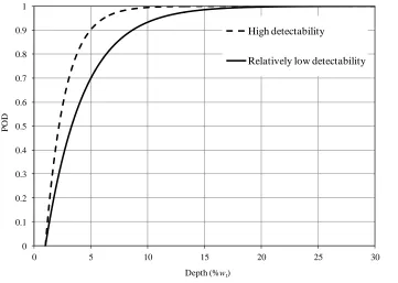
2.2.2 Probability of detection and probability of false call

POD represents the ability of an ILI tool to detect a true corrosion defect. It is

typically a function of the size of the defect and a set of parameters indicating the

inherent detecting capability of the ILI tool. The following exponential POD function

(Zheng and Ellingwood 1998) was adopted in this study:

(2.3)

where x denotes the actual depth of a given defect; xth denotes the detection threshold, i.e.

the smallest defect size that can be detected, and q is a constant that characterizes the

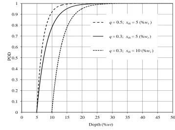
inherent detecting capability of the ILI tool. Figure 2.1 shows the POD curves given by

Eq. (2.3) with three sets of values of q (1/%wt) and xth (%wt), where %wt represents the

percentage of the pipe wall thickness (wt). This figure indicates that the detectability of

the tool increases as the value of q increases and/or the detection threshold xth decreases.

The probability of false call (POFC) is the probability of an ILI tool obtaining an

indication of a defect that does not exist in reality. For the high-resolution ILI tools

(26)

Therefore, POFC was ignored in the present study; in other words, all the ILI-reported

corrosion defects were assumed to be true corrosion defects.

Figure 2.1 POD curves with different sets of values of q and xth

2.3 Probabilistic Models for Defect Generation and Growth

2.3.1 Defect generation

The non-homogeneous Poisson process (NHPP) was employed to characterize the

generation of new defects, as the model has been widely used in the literature (e.g. Valor

et al. 2007; Kuniewski et al. 2009). According to this model, the total number of defects,

N(t), generated within a time interval [0, t] (e.g. t = 0 denotes the time of installation of

the pipeline) over a given segment of the pipeline follows a Poisson distribution with a

probability mass function (PMF), fP(N(t)|m(t)), defined as (Beichelt and Fatti2002)

(t ≥ 0) (2.4)

0 0.1 0.2 0.3 0.4 0.5 0.6 0.7 0.8 0.9 1

0 5 10 15 20 25 30 35 40 45 50

P

O

D

Depth (%wt)

q= 0.5; xth= 5 (%wt)

q= 0.3; xth= 5 (%wt)

(27)

where m(t) denotes the expected number of defects generated over the time interval [0, t],

and is assumed in this study to follow a power-law function of time (Kuniewski et al.

2009): with the parameters  and  (,  > 0) to be

quantified based on the inspection data. Figure 2.2 depicts the means, 2.5- and

97.5-percentile values, and realizations of N(t) over 20 years based on Eq. (2.4) corresponding

to two sets of assumed values of λ and δ. Note that N(t) degenerates to a homogeneous

Poisson process (HPP) if  equals unity.

Figure 2.2 Mean, 2.5-percentile, 97.5-percentile and a given realization of NHPP

Suppose n inspections have been carried out for a given pipeline segment over a

certain period of time. It is assumed that each inspection is able to identify new and

existing corrosion defects by tracking their spatial positions. This assumption is

consistent with the corrosion inspection practice for oil and gas pipelines (Al-Amin et al.

2012). At the time of the ith inspection (i = 1, 2, ..., n), ti, the total number of corrosion

defects on the pipeline segment, Ni, can be divided into those defects that have initiated

prior to the (i-1)th inspection, Nio, and those defects that initiated between the (i-1)th and

0 20 40 60 80 100 120 140 160 180 200

0 2 4 6 8 10 12 14 16 18 20

N um be r of d ef ec ts Time (year) 97.5- percentile Mean 2.5- percentile Realization

λ= 2; δ= 1.5

(28)

ith inspections, Nig. The quantity Nig then follows a Poisson distribution with a PMF

given by

(2.5)

where

, and t0 0.

Because of the imperfect detectability of the ILI tool, the detected number of defects is

in general less than the actual number of defects. Let Nigd and Nigu denote the detected

and undetected portions of Nig, respectively, i.e. Nig = Nigd + Nigu. Based on the Poisson

splitting property (Kulkarni 1995), Nigd and Nigu follow Poisson distributions with the

corresponding PMFs as follows:

=

(2.6)

=

(2.7)

where is the average POD with respect to the Nig defects. can be calculated

as , where is the PDF of the depths of defects at

time ti.

2.3.2 Defect growth

The non-homogeneous gamma process (NHGP) (Zhang et al. 2014) was employed to

characterize the growth of depths of corrosion defects. It follows that the depth of a

given defect at time t, X(t), is gamma distributed with the PDF given by:

(2.8)

where α(t) is the time-dependent shape parameter and assumed to be a power-law

(29)

(the time at which a defect initiates and starts growing); β (β > 0) is the time-independent

rate parameter (or inverse of the scale parameter) (Ang and Tang 2007); Γ(∙) denotes the gamma function, and I(0,∞)(x(t)) is the indication function, which equals unity if x(t) > 0

and zero otherwise. The mean, variance and coefficient of variation (COV) of X(t) equal

α(t)/β, α(t)/β2 and 1/(α(t))0.5, respectively. The quantity φ1/β represents the mean of the

depth at the first unit increment of time since ts; φ2 reflects the slope of the mean growth

path of the defect with φ2 > 1, φ2 < 1 and φ2 = 1 representing an accelerating, a

decelerating and a linear mean growth path, respectively. Furthermore, φ2 = 1

corresponds to a homogeneous gamma process.

In this study, the parameters φ1 and φ2 were assumed to be common for all the defects,

whereas ts and β were assumed to be defect-specific to account for the spatial variability

of the defect growth. Let tsr and βr denote the time of initiation and rate parameter for the

rth defect(r = 1, 2, ...), respectively. It should be emphasized here that the index r is used

to enumerate all defects, including detected and undetected defects, to distinguish from

the index j that is used to enumerate detected defects. The parameter βr was further

assumed to be an exponential function of the random effect parameter ξr, i.e. βr = .

The advantage of expressing βr as an exponential function is that it ensures βr to be

positive and can easily incorporate local covariates, if any, to more accurately

characterize βr.

It follows from the above-described assumptions that the depth increment of defect r

over the time interval between the (i-1)th and ith inspections, denoted by Δxir, is

gamma-distributed with a shape parameter Δαir and a rate parameter βr, where Δαir is given by

(2.9)

The depth of defect r at the ith inspection, xir, is then the summation of the depth at the

(i-1)th inspection and Δxir; that is, xir = xi-1, r + Δxir. Note that xir at t = tsr is assumed to

(30)

2.4 Bayesian Updating of Defect Generation and Growth Models

2.4.1 Overview

The Bayesian updating was employed to make statistical inferences of the parameters of the defect generation and growth models described in Section 2.3 based on the ILI data. Through Bayes' theorem, the Bayesian updating combines the previous knowledge about uncertain model parameters with the new information contained in the observed data to lead to updated knowledge about these parameters. The previous knowledge is reflected in the prior distributions; the new information in the observed data is incorporated in the likelihood functions, and the updated knowledge of the parameters is reflected in the posterior distributions. The formulations of the prior and posterior distributions as well as the likelihood functions for the defect generation and growth models are described in the following sections.

2.4.2 Likelihood functions

2.4.2.1 Likelihood function for ILI-reported depths

Consider that a set of defects have been detected in a total of n inspections. Suppose

that defect j is first detected in the lth (l = 1, 2, ..., or, n) inspection. Let yj = (ylj, yl+1,j, …,

yl+k,j, …, ynj)' denote the vector of the ILI-reported depths for defect j. Further let xj = (xlj,

xl+1,j, …, xl+k,j, …, xnj)' denote the vector of the actual depths of defect j corresponding to

the ILI-reported depths. Given the measurement error model described in Section 2.2.1,

the likelihood of yj conditional on xj can be expressed as

(2.10)

where a = (al, al+1, …, an)', and b is an n-l+1 × n-l+1 diagonal matrix with the kth element

equals to bl+k. The above formulation assumes that once a defect is detected for the first

time, it will be detected in all subsequent inspections. It should be noted that this

assumption can be relaxed in the analysis; that is, the defect is not necessarily detected in

all subsequent inspections. In this case, the ILI-reported depths corresponding to the

(31)

handled using the multiple imputation technique (Rubin 2009), which has been

implemented in widely used Bayesian updating software such as OpenBUGS (Lunn et al.

2009).

2.4.2.2 Likelihood function for the number of detected defects

To simplify the likelihood functions for the number of defects, it is assumed that the

defects detected for the first time (referred to as the newly detected defects) in the ith

inspection are generated between the (i-1)th and ith inspections. This assumption ignores

the possibility that some of the newly detected defects in the ith inspection may in fact

initiate prior to the (i-1)th inspection but remain undetected until the ith inspection. The

assumption results in overestimation of the intensity of the defect generation. It follows

from the assumption that the newly detected defects in the ith inspection can be denoted

by Nigd as defined in Section 2.3.1. Based on this assumption and Eq. (2.6), the

likelihood function for the set of newly detected defects in n inspections, i.e. Nigd (i = 1,

2, …, n), is given by

(2.11)

Note that the evaluation of involves the depths of both detected and undetected

defects in the ith inspection. The depths of undetected defects were treated as the missing

data and handled using the data augmentation (DA) technique (Tanner and Wong 1987),

which is described in Section 2.4.4. It follows that serves as a link between the

defect generation and growth models in the Bayesian updating.

2.4.3 Prior distributions

The gamma distribution was selected as the prior distribution for parameters λ and δ of

the NHPP-based defect generation model, and for parameters φ1 and φ2 of the

(32)

ensures these parameters to be positive and can be conveniently constructed to be

non-informative. Consistent with the assumption stated in Section 2.4.2.2, the prior

distribution for the initiation time of a given detected defect j, tsj, was selected to be

uniformly distributed with the corresponding upper bound (ubj) equal to the time of the

inspection that detects the defect for the first time and the lower bound (lbj) equal to the

time of the immediate previous inspection. The prior distributions for tsj for different

defects were further assumed to be mutually independent. The random effect parameter

ξr corresponding to different defects were assumed to follow independent identical (iid)

normal prior distributions with a mean of zero and a common uncertain variance σ2. The

hierarchical structure for ξr facilitates the generation of the depths of undetected defects

as required by the data augmentation analysis. Finally, the prior distribution for 1/σ2was

assigned a gamma distribution (i.e. σ2 follows an inverse-gamma distribution) as

commonly suggested in the literature (e.g. Ntzoufras 2011), which leads to the conjugate

posterior distribution for 1/σ2 and can improve the computational efficiency. The shape

(rate) parameters of the gamma prior distributions for φ1, φ2, ,  and 1/σ2 are denoted by

c (d), e (f), g (h), (η) and (), respectively.

2.4.4 Posterior distributions, MCMC simulation and missing data

Because it is not possible to analytically derive the complex joint posterior distribution of the parameters of the defect generation and growth models, the Markov chain Monte Carlo (MCMC) simulation techniques (Gilks 2005) were employed to numerically evaluate the joint posterior distribution of the model parameters. A hybrid algorithm combining the Metropolis-Hastings (M-H) algorithm and Gibbs sampling (Tierney 1994)

was implemented in MatlabTM to carry out the MCMC simulation. The derivations of

full conditional posterior distributions of the model parameters as required by the hybrid algorithm are included in Appendix 2A. It is emphasized that both the detected and undetected defects were incorporated in the Bayesian updating. The actual depths of the

detected defects are related to the ILI-reported depths through the likelihood function

given by Eq. (2.10), whereas the actual depths of the undetected defects were treated as

the missing data and imputed using the DA technique (Tanner and Wong 1987).

(33)

depths of the overall defect population as opposed to the depths of the detected defect

population only.

DA is an iterative process and can be straightforwardly incorporated in the MCMC

simulation. A given DA iteration includes two steps, namely the imputation step and the

posterior step (Little and Rubin 2002). The former is used to generate the samples of the

missing data from its corresponding probabilistic distribution conditional on the current

state of model parameters, and the latter is used to generate a new set of samples of

model parameters from their corresponding posterior distributions conditional on both the

observed and missing data. Details of the DA technique can be found in Little and Rubin

(2002).

A step-by-step procedure for generating samples of the model parameters as well as

samples of the missing data (i.e. depths of undetected defects) in the kth (k = 1, 2, ...)

MCMC simulation sequence is described as follows, where the notation (k) is used to

denote the value of  obtained in the kth simulation sequence.

1. Impute depths of undetected defects (i.e. missing data).

1.1) Generate the number of undetected defects initiated between the (i-1)th and ith (i

= 1, 2, …, n) inspections, i.e. Nigu(k), from the Poisson PMF given by Eq. (2.7) with ,

 and replaced by (k-1), (k-1) and , respectively.

1.2) Generate depths of Nigu(k) undetected defects, , (v = 1, 2, ..., Nigu(k)) as follows.

1.2.1) Set v = 0;

1.2.2) generate a random effect parameter (k) from the normal distribution with a

zero mean and a variance of σ2(k-1), and then calculate (k) = ;

1.2.3) generate a defect initiation time ts(k) based on the procedure described in

Appendix 2B.

(34)

2, ts and  equal to 1(k-1), 2(k-1), ts(k) and (k), respectively;

1.2.5) if x is less than the detection threshold of the ILI tool, i.e. xth, accept x as

the depth of an undetected defect; otherwise, accept x with a probability of 1 -

POD(x);

1.2.6) set v= v + 1 if x is accepted, and

1.2.7) repeat Steps 1.2.2) through 1.2.6) until v = Nigu(k).

2. For the set of Nigd defects (i = 1, 2, ..., n), i.e. the newly detected defects in the ith

inspection, generate the corresponding depths at the ith and all subsequent inspections,

(l = i, i + 1, ..., n; j = 1, 2, ..., Nigd) as follows:

2.1) generate the increments of the depth between consecutive inspections for each of

the Nigd defects, , from the full conditional posterior distribution listed in

Appendix 2A using the M-H algorithm, and

2.2) calculate for j = 1, 2, ..., Nigd.

3 Calculate for i = 1, 2, ..., n as follows:

. (2.12)

4 Sample (k), (k), 1(k), 2(k), tsj(k), j(k) (j = 1, 2, ..., ) and σ2(k) from the

corresponding full conditional posterior distributions listed in Appendix 2A using either

the M-H algorithm or Gibbs sampling.

2.5 Illustrative Examples

2.5.1 Example 1

In the first example, we used hypothetical (i.e. simulated) inspection data to illustrate

(35)

defect generation and growth models were set to be deterministic quantities with  = 2, 

= 1.2, 1 = 3 and 2 = 0.9, and the random effect parameter  for different defects was

assumed to follow iid normal distributions with a zero mean and σ2 = 0.36. It is assumed

that three inspections were carried out after the installation of the pipeline (t = 0) with ti =

i × 5 years (i = 1, 2 and 3). For simplicity, the constant and non-constant biases included

in the measurement error model given by Eq. (2.1) were set to equal zero and unity,

respectively, for all the inspections, and the random scattering errors associated with

different inspections were assumed to be mutually independent with the same standard

deviation of unity. Finally, the POD functions associated with all the inspections were

assumed to be identical, with the parameters q and xth set to be q = 0.30 (1/%wt) and xth =

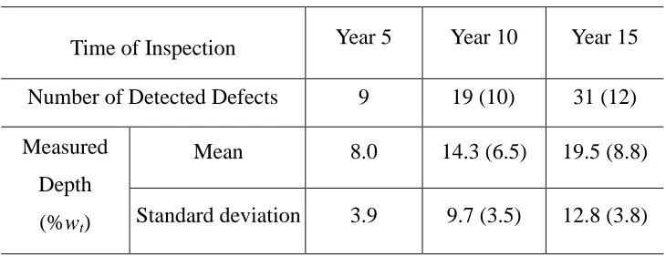
1 (%wt). Table 2.1 summarizes the simulated inspection data, whereby the simulation

procedure is described in Appendix 2C. Note that the simulation is based on the

assumption stated in Section 2.4.2.2, i.e. the newly detected defects in the ith inspection

are all generated between the (i-1)th and ith inspections.

Table 2.1 Summary of the simulated inspection data

Time of Inspection Year 5 Year 10 Year 15

Number of Detected Defects 9 19 (10) 31 (12)

Measured

Depth

(%wt)

Mean 8.0 14.3 (6.5) 19.5 (8.8)

Standard deviation 3.9 9.7 (3.5) 12.8 (3.8)

Note: The information for newly detected defects in years 10 and 15 year is in brackets.

The Bayesian updating was carried out to evaluate the parameters of the defect generation and growth models based on the simulated inspection data. The shape and scale parameters of the gamma prior distributions for , , 1 and 2 were set to be unity,

and the shape and scale parameters of the inverse-gamma prior distribution for σ2 were

set to be 10. A total of 100,000 MCMC simulation sequences were generated following

(36)

sequences were used to evaluate the probabilistic characteristics of the model parameters.

The means, medians and standard deviations of the posterior marginal distributions of the

model parameters that are common to all the defects are summarized in Table 2.2, where

, and denote the average POD for the defects generated prior to year 5,

between years 5 and 10, and between years 10 and 15, respectively. The results in Table

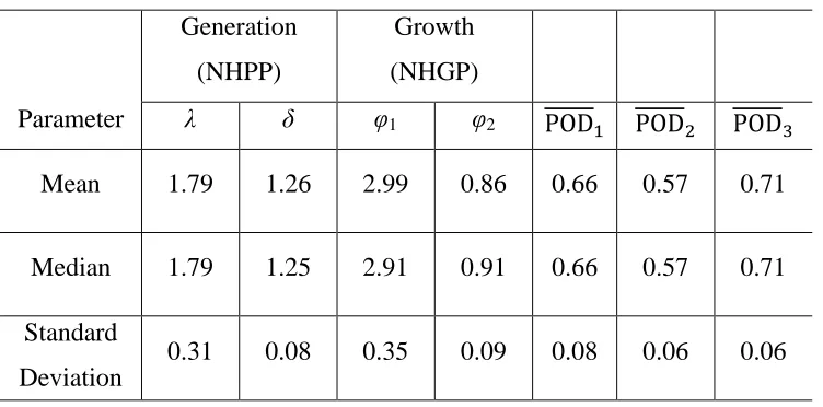
2.2 suggest that the posterior mean and median values of , , 1 and 2 are in good

agreement with the corresponding actual values.

Table 2.2 Posterior statistics of model parameters for Example 1

Parameter

Generation

(NHPP)

Growth

(NHGP)

λ δ φ1 φ2

Mean 1.79 1.26 2.99 0.86 0.66 0.57 0.71

Median 1.79 1.25 2.91 0.91 0.66 0.57 0.71

Standard

Deviation

0.31 0.08 0.35 0.09 0.08 0.06 0.06

To investigate the impact of undetected defects on the outcome of the Bayesian

updating, two additional scenarios were considered. Scenario I assumes perfect

detectability associated with all three inspections (i.e. no undetected defects), whereas

Scenario II considers POD but includes only the detected defects (i.e. ignoring the

missing data) in calculating (i = 1, 2 and 3) and updating the growth model. In

contrast, the results summarized in Table 2.2 are referred to as the base case. The MCMC

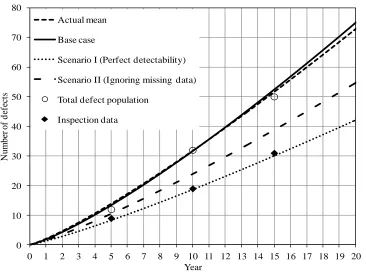
simulation was carried out for Scenarios I and II. For the base case and Scenarios I and II,

the mean values of the number of generated defects, i.e. m(t) = tδ, were then calculated

for 0 ≤ t ≤ 20 years, where the values of  and δ were set to the corresponding posterior

medians. The results are shown in Fig. 2.3. For comparison, m(t) evaluated from the

actual values of  and δ, the simulated total numbers of defects (including the detected

and undetected defects) at the times of the three inspections, as well as the simulated

(37)

indicated in the figure, m(t) corresponding to the base case is practically identical to the

actual mean and agree well with the total number of defects, whereas both Scenarios I

and II lead to underestimated m(t) values with the degree of underestimation increasing

with time. The values of m(t) corresponding to Scenario I at t = 5, 10 and 15 years agree

well with the inspection data. This is expected because perfect detectability is assumed

for Scenario I. The m(t) curve corresponding to Scenario II lies in between those

corresponding to Scenario I and the base case. This is because although POD is

accounted for in Scenario II, is overestimated as a result of ignoring the missing

data in the calculation.

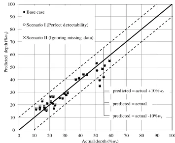
For the base case and Scenarios I and II, the depths of the detected defects at year 20

were predicted and compared with the corresponding actual defect depths. The predicted

depth for a given defect was selected as the mean depth predicted from the NHGP-based

growth model, with values of the model parameters (i.e. 1, 2, tsj and ξj) set to the

corresponding posterior medians. The results are shown in Fig. 2.4. Figure 2.4 suggests

that all three cases predict the growth of corrosion defects reasonably well: the predicted

depths for 90% of the 31 detected defects fall between the two bounding lines of actual

depth 10%wt. The differences between the predictions corresponding to the three cases

are marginal: the predictions for relatively shallow defects (say, depth ≤ 30%wt)

corresponding to Scenarios I and II tend to be slightly higher than those corresponding to

(38)

Figure 2.3 Comparison of predicted numbers of defects corresponding to the base case

and Scenarios I and II

As described in Section 2.4.2.2, the Bayesian methodology developed in this study

involves the simplifying assumption that the newly detected defects in the ith inspection

are all generated between the (i-1)th and ith inspections. To investigate the impact of this

assumption on the predictive capability of the proposed methodology, we further

simulated more realistic corrosion data considering the possibility that some of the newly

detected defects in the ith inspection may in fact initiate prior to the (i-1)th inspection but

remain undetected until the ith inspection. These data were then used to update the

corrosion generation and growth models and make predictions. 0

10 20 30 40 50 60 70 80

0 1 2 3 4 5 6 7 8 9 10 11 12 13 14 15 16 17 18 19 20

N

um

be

r

of

d

ef

ec

ts

Year Actual mean

Base case

Scenario I (Perfect detectability)

Scenario II (Ignoring missing data)

Total defect population

(39)

Figure 2.4 Comparison of the predicted and actual depths at year 20

The corrosion inspection data at years 5, 10 and 15 were simulated based on the same

set of parameters as those used to generate the data summarized in Table 2.1 except for

the POD curve. Three different POD curves were considered in this case, corresponding

to POD of 90%, 70% and 50%, respectively, for a defect depth of 5%wt with a detection

threshold of 1%wt. The simulated inspection data corresponding to the three different

POD curves are summarized in Table 2.3. The simulation procedure is described in

Appendix 2D.

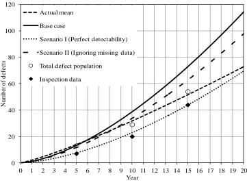
The Bayesian updating was then carried out corresponding to the base case, Scenarios

I (i.e. perfect detectability) and II (i.e. ignoring the missing data in evaluating the average

POD). The mean values of the number of generated defects, i.e. m(t) = tδ, were

calculated for 0 ≤ t ≤ 20 years, where the values of  and δ were set to the corresponding

posterior medians. The results are shown in Figs. 2.5 in a similar fashion as those shown

in Fig. 2.3. 0 10 20 30 40 50 60 70 80 90 100

0 10 20 30 40 50 60 70 80 90 100

Base case

Actual depth (%wt)

P re d ic te d d ept h (% wt )

predicted = actual +10%wt

predicted = actual

(40)

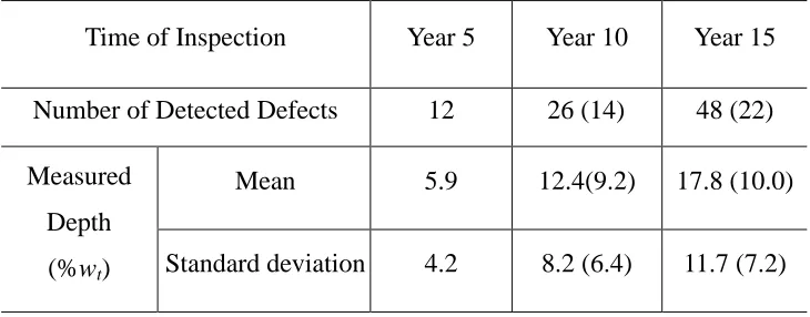
Table 2.3 Summary of the simulated inspection data corresponding three different

POD curves

(a) POD = 90% for a defect depth of 5%wt

Measured

Depth

(%wt)

Mean 5.9 12.4(9.2) 17.8 (10.0)

(b) POD = 70% for a defect depth of 5%wt

Measured

Depth

(%wt)

Mean 8.0 14.1 (10.4) 18.8 (12.5)

(c) POD = 50% for a defect depth of 5%wt

Measured

Depth

(%wt)

Mean 7.0 14.1(11.7) 18.3 (12.1)

(41)

(a) POD of 90% for a defect depth of 5%wt

(b) POD of 70% for a defect depth of 5%wt 0 10 20 30 40 50 60 70 80 90 100

0 1 2 3 4 5 6 7 8 9 10 11 12 13 14 15 16 17 18 19 20

N um be r of d ef ec ts Year Actual mean Base case

Inspection data 0 10 20 30 40 50 60 70 80 90 100

0 1 2 3 4 5 6 7 8 9 10 11 12 13 14 15 16 17 18 19 20

N um be r of d ef ec ts Year Actual mean Base case

(42)

(c) POD of 50% for a defect depth of 5%wt

Figure 2.5 Comparison of predicted numbers of defects corresponding to the base case

and Scenarios I and II based on more realistic corrosion inspection data

As indicated in Fig. 2.5, the m(t) curves corresponding to the base case overestimate

the total number of defects. The degree of overestimation decreases as the detectability

of the inspection tool increases. This is because the higher is the detectability of the

inspection tool, the smaller portion of the newly detected defects are previously

undetected defects and the smaller impact does the simplifying assumption have on the

prediction. It is interesting to note that the m(t) curves corresponding to Scenario II agree

with the total defect population better than those corresponding to the base case and

Scenario I. This is because ignoring the missing data in calculating the average POD in

Scenario II leads to overestimation of the average POD and underestimation of the total

number of defects, which somewhat offsets the overestimation of the total number of

defects due to the simplifying assumption that the newly detected defects in the ith

inspection are all generated between the (i-1)th and ith inspections. It should be pointed

out that the POD assumptions corresponding to Figs. 2.5(a) and 2.5(b) are more 0

20 40 60 80 100 120

0 1 2 3 4 5 6 7 8 9 10 11 12 13 14 15 16 17 18 19 20

N

um

be

r

of

d

ef

ec

ts

Year Actual mean

Base case

(43)

representative of the inspection tools commonly used in the pipeline industry than that

corresponding to Fig. 2.5(c). For the former two assumptions, the conservatism in the

predictions associated with the base case is relatively small.

2.5.2 Example 2

In the second example, real ILI data collected from a pipe joint (approximately 13.6m

long) in a natural gas pipeline located in Alberta were used to illustrate the proposed

methodologies. The pipeline was constructed in 1972 and inspected by high-resolution

magnetic flux leakage (MFL) tools in 2004, 2007 and 2009. Note that the pipeline had

also been inspected prior to 2004; however, the corresponding inspection data are not

available to the present study. The numbers of defects on the pipe joint considered and

the statistics of the corresponding defect depths reported by the ILIs in 2004, 2007 and

2009 are summarized in Table 2.6.

The measurement errors associated with the three ILI tools as well as the correlation

between the random scattering errors associated with different ILI tools were quantified

using the Bayesian methodology in a previous study (Al-Amin et al. 2012). The

calibrated biases, the random scattering errors as well as the correlations between the

random scattering errors are as follows: a1 = 2.04 (%wt) , a2 = -15.28 (%wt), a3 = -10.38

(%wt), b1 = 0.97, b2 =1.40, b3 = 1.13; 1 = 5.97 (%wt), 2 = 9.05 (%wt) and 3 = 7.62

(%wt); 12 = 0.70, 13 = 0.72 and 23 = 0.78 (Al-Amin et al. 2012), where the subscripts

‘1’, ‘2’ and ‘3’ denote the parameters associated with the ILI tools used in 2004, 2007 and

2009, respectively. The above-mentioned measurement errors were quantified based on

128 defects that were located on several pipe joints in the same pipeline considered in

this example, but were mitigated and ceased growing prior to 2000.

The actual POD functions associated with the ILI tools are unavailable. We therefore

assumed the three ILI tools to have the identical exponential POF function given by Eq.

(2.3). The detection threshold xth in Eq. (2.3) was assumed to be 1 (%wt), whereas the

parameter q was characterized for both the high and relatively low detectability

assumptions. The former corresponds to a POD of 90% for a defect depth of 5%wt,