On the Cryptographic Hardness of Finding a Nash Equilibrium

(1)

On the Cryptographic Hardness of Finding a Nash Equilibrium

Nir Bitansky∗ Omer Paneth† Alon Rosen‡ August 14, 2015

Abstract

We prove that finding a Nash equilibrium of a game is hard, assuming the existence of indistin-guishability obfuscation and one-way functions with sub-exponential hardness. We do so by showing how these cryptographic primitives give rise to a hard computational problem that lies in the complexity class PPAD, for which finding Nash equilibrium is complete.

Previous proposals for basing PPAD-hardness on program obfuscation considered a strong “virtual black-box” notion that is subject to severe limitations and is unlikely to be realizable for the programs in question. In contrast, for indistinguishability obfuscation no such limitations are known, and recently, several candidate constructions of indistinguishability obfuscation were suggested based on different hardness assumptions on multilinear maps.

Our result provides further evidence of the intractability of finding a Nash equilibrium, one that is extrinsic to the evidence presented so far.

∗

MIT. Email:[email protected]. †

Boston University. Email: [email protected]. Supported by the Simons award for graduate students in theoretical computer science and an NSF Algorithmic foundations grant 1218461.

‡

(2)

1 Introduction

The notion ofNash equilibriumis fundamental to game theory. While a mixed Nash equilibrium is guar-anteed to exist in any game [Nas51], there is no known polynomial-time algorithm for finding one. The tractability of the problem has received much attention in the past decade, in large part due to its theo-retical and philosophical significance. Prominent evidence for the hardness of finding a Nash equilibrium emerges from a line of works, originating in Papadimitriou [Pap94] and ultimately showing that the prob-lem is complete for the complexity class PPAD [DGP09, CDT09]. The class PPAD contains several other search problems that are not known to be tractable, such as finding a fixed point of the kind guaranteed by Brouwer’s Theorem. Akin to the phenomenon of NP-completeness, this could be interpreted as evidence to computational difficulty. However, unlike in the case of NP, currently known problems in PPAD appear to be of fairly restricted nature, and carry similar flavor to one another.

Seeking further evidence for the hardness of PPAD, we aim to to base its hardness on new types of problems. As observed in [MP91, Pap94] problems in PPAD cannot be NP-complete unless NP = coNP, since the class istotal. A potential source for such problems, already pointed out in [Pap94], iscryptographic hardness. Indeed, many classical cryptographic problems are believed to reside “on the boundary of P”; namely, they are believed to be hard, but not NP-hard. (Indeed, for some total super-classes of PPAD such as PPA and PPP hardness is known based on factoring or collision-resistant hashing, respectively [Jeˇr].)

Towards identifying a suitable problem from the domain of cryptography, let us first take a closer look into the definition of PPAD. The class PPAD consists of all total search problems reducible to the following END-OF-THE-LINEproblem. We are given a program succinctly representing an exponential size directed graph over the nodes{0,1}n_{, together with a source node}_x

s. The in-degree and out-degree of every node

are at most one, and the in-degree of the sourcexsis zero. Our goal is to find another node, other thanxs,

with in-degree or out-degree zero. Such a node must exist by a simple parity argument.

Intuitively, solving theEND-OF-THE-LINEproblem appears to require some sort of ”reverse-engineering” of the program representing the graph. Indeed, under minimal cryptographic assumptions, solving the prob-lem while only treating the program as a black-box is impossible. For instance, the program may internally invoke a pseudo-random permutation [LR88] to describe a “random looking”END-OF-THE-LINEgraph that cannot be solved efficiently with only black-box access.1

This suggests a natural approach for constructing PPAD-hard problems based oncryptographic obfus-cation, a compiler that transforms any program into an unintelligible one while preserving functionality. Ideally, an obfuscated program should be equivalent to a virtual black-box (VBB): it should reveal nothing more than what can be learned from its input-output behavior [BGI+01]. In particular, a (pseudo) ran-domEND-OF-THE-LINEgraph described by an obfuscated program should be unsolvable by any efficient algorithmeven given this obfuscated program. Abbot, Kane and Valiant [AKV04] further show that PPAD-hardness can be based on VBB obfuscation of an even simpler program that essentially computes some natural pseudo random function.

Neither of the above programs, however, is known to be VBB obfuscatable. Indeed, VBB obfuscation is currently known only for a few simple functions based on strong assumptions. Moreover, certain functions are impossible to VBB obfuscate [BGI+01], and VBB obfuscation of pseudo-random functions, including the one considered in [AKV04], is in particular subject to strong limitations [GK05, BCC+14].

In light of the impossibilities for VBB obfuscation, Barak et al. [BGI+01] defined indistinguishabil-ity obfuscation(iO), a relaxed notion requiring only that the obfuscations of any two equal-size circuits computing the same function are indistinguishable from one another. For iO, no impossibilities are known.

1

(3)

Furthermore, starting with the work of Garg et al. several constructions of iO were recently suggested based on different assumptions related to cryptographic multilinear maps [GGH+13, BR14, BGK+14, PST14, GLSW14, Zim14, AB15, AJ15, BV15]. A natural question is whether the comparatively weak security guarantees of iO suffice for establishing hardness of PPAD.

1.1 This Work

We show PPAD-hardness based on indistinguishability obfuscation and one-way functions with super-polynomial hardness.

Theorem 1.1(Informal). Suppose that there exist sub-exponentially-hard injective one-way functions and quasi-polynomially-hard indistinguishability obfuscation for P/poly. Then theEND-OF-THE-LINEproblem is hard for polynomial-time algorithms.

In fact, under the above assumptions, we show that PPAD is hard on average for quasi-polynomial algorithms. Specifically, there exists an efficiently-samplable distribution onEND-OF-THE-LINEinstances that fails probabilistic quasi-polynomial algorithms (for some quasi-polynomial function that depends on the iO hardness). We can get sub-exponential PPAD-hardness at the cost of assuming sub-exponential iO. We can also trade-off the security of the iO and the resulting PPAD-hardness with the security of the one-way function. Specifically, we show that assuming only polynomially-hard iO, but exponentially-hard injective one-way functions, PPAD is hard in the worst-case (rather than on average) for polynomial-time algorithms. We also note that the assumption of sub-exponentialinjectiveone-way functions can be traded with sub-exponential iO and sub-exponential (non-injective) one-way functions [BPW15], and the latter can be further traded with the assumption that NTime(2O(nε))6=ioBPTime(2O(nε))[KMN+14].

While we mainly interpret our result as evidence for the hardness of PPAD, one may also consider a converse interpretation: any algorithmic breakthrough resulting, say, in a sub-exponential algorithm for computing Nash equilibria will lead to a sub-exponential attack on the hardness of iO or one-way functions.

1.2 Main Ideas

To demonstrate the hardness of PPAD, we construct a hard distribution overEND-OF-THE-LINEinstances. Recall that anEND-OF-THE-LINEinstance is defined by a program representing an exponential size directed graph. Verifying that a given program indeed describes a validEND-OF-THE-LINE instance can be done efficiently (thus making the problem total [MP91, Pap94]).

In more detail, anEND-OF-THE-LINEgraph is described by a pair of circuitsSandP. Given an input node x ∈ {0,1}n_, _S₍_x₎ _{outputs a “candidate successor” and} _P₍_x₎ _{outputs a “candidate predecessor” of}

x. We say that there is an edge from x tox0 in the graph if S(x) = x0 andP(x0) = x (this guarantees that the in-degree and out-degree of every node are at most one). The instance also defines a source node

xs ∈ {0,1}nand we require thatP(xs) =xs6=S(xs)(this guarantees that the in-degree of the source node

xsis zero). The solution is any node other thanxswith in-degree or out-degree zero.

A simplified construction.To convey the main ideas behind the hardness proof, we first describe a simpli-fied construction ofEND-OF-THE-LINE instances that will only satisfy a weak form of hardness, and then extend it to obtain the sought-after result. In the constructed (distribution over) instances, the circuits S

andPcontain the description a functionPRF : [T] → {0,1}m _{sampled from a family of pseudo-random}

functions, whereT is of super-polynomial size.

Nodesxin the graph are of the form(i, σ) ∈[T]× {0,1}m_{. We say that a node}₍_{i, σ}₎_is_valid_if_σ ₌

(4)

node will be connected to itself by a self-loop. The graph contains a single source nodexs = (1,PRF(1))

with in-degree zero and a single sink node(T,PRF(T))with out-degree zero. Given a node(i, σ), the circuitScomputes the candidate successor as follows:

1. If the node is valid andi < T,Soutputs the node(i+ 1,PRF(i+ 1))as the candidate successor.

2. If the node is invalid or ifi=T,Soutputs the node(i, σ)unchanged.

The functionPis defined analogously in the reverse direction. TheEND-OF-THE-LINEinstance is the triplet

(˜S,P˜,(1,PRF(1))), whereS˜andP˜ are indistinguishability obfuscations of the circuitsSandPrespectively and(1,PRF(1))is the source node. Note that this instance has a unique solution(T,PRF(T)).

Intuition.The path from the source(1,PRF(1))to the sink(T,PRF(T))should be thought of as an authen-ticated chain where a signatureσcorresponding to some valid node(i, σ)cannot be obtained without first obtaining all previous signatures. It is not difficult to show that any efficient algorithm that only invokes the circuitsSandP(and thus also the pseudo-random functionPRF) as a black box cannot find the signature

PRF(T), and thus cannot solve the instance. We would like to prove that the same hardness holdseven given the obfuscated circuits˜SandP˜. However, we first prove something weaker:finding the sink(T,PRF(T))is hard given only the successor circuit˜S. We then extend the proof to show that the sink is hard to find given

bothS˜andP˜, which requires modifying the construction.

To prove that finding the signaturePRF(T)corresponding to the sink is hard, we show that the obfus-cated˜Sis computationally indistinguishable from a circuit that on input (T,PRF(T))returns some fixed value⊥, rather than(T,PRF(T))itself as˜Swould. This implies that an efficient algorithm would not be able to obtainPRF(T)from either one of the circuits, or it could distinguish the two. We next go in more detail into how indistinguishability of these two circuits is shown.

For everyj ≤k≤T, we consider the circuitSj,kthat is identical toS, except that for everyi∈[j, k],

Sj,k on the input (i,PRF(i)) outputs the fixed value ⊥. The argument proceeds in two steps. First, we

show that for arandomu ∈ [T], an obfuscationS˜u,u ofSu,uis computationally indistinguishable from˜S.

Intuitively this “splits” the authenticated chain into two parts. While given the source node it is possible to compute additional signatures in the first part of the chain [1, u−1], we show that is it hard to find a signature for any iin the second part of the chain[u, T]. More concretely, in the second step, we prove that the obfuscated circuitsS˜u,u and˜Su,T are computationally indistinguishable by a sequence of hybrids.

For every j ∈ [u, T], we show that the obfuscations ˜Su,j and ˜Su,j+1 are computationally

indistinguish-able. In total, we haveT hybrids; relying on injective one-way functions (which come up in the analysis) and iO with super-polynomial hardness (related to the size ofT), we show that each two obfuscations are

T−Θ(1)-indistinguishable. Overall we deduce that the obfuscationsS˜ and ˜Su,T are also computationally

indistinguishable as required. To summarize, the hardness proof follows two steps:

1. Split the chain into two parts:For a randomu∈[T], prove that˜SandS˜u,T are indistinguishable.

2. Erase second part:For everyu≤j < T, prove thatS˜u,jand˜Su,j+1areT−Θ(1)-indistinguishable.

We next explain how two the steps described above are proven. For simplicity, we shall assume the existence of a length-doubling pseudo-random generatorPRG: [T]→[T2]that is injective; in the body, we relax this assumption and rely only on injective one-way functions (which as noted above can be constructed from plain one-way functions and iO). The two steps rely the ideas ofhidden triggers and punctured programs

introduced by Sahai and Waters [SW14].

First step. To prove thatS˜is indistinguishable from˜Su,u, we first note thatS˜is indistinguishable from an

(5)

1. ifσ=PRF(i)andPRG(i) =v, return⊥.

2. Otherwise return(i+ 1,PRF(i+ 1))(asSwould);

here v is chosen at random from the range [T2]of PRG. Observe that, with overwhelming probability 1− 1

T, v is not in the image of PRG, the condition in (1) is never met, and the alternative behavior is

never triggered. Thus, S andSv compute the same function and their obfuscations are indistinguishable.

Next, relying on the pseudo-randomness guarantee ofPRG, we can indistinguishably replace the uniformly randomv with a pseudo-random valuePRG(u). It is left to note that, because PRGis injective,Sv, with

v = PRG(u), computes the exact same function asSu,u. Indeed, both compute the same function as S

except on(u,PRF(u)), where an alternative behavior is triggered and⊥is returned.

Second step. To prove that˜Su,jandS˜u,j+1are indistinguishable, we require thatPRFispuncturable. This

means that for every inputi∈ [T], we can sample a puncturedPRF{i} that agrees withPRFon all inputs

j 6=i, but computationally hides any information on the valuePRF(i); namelyPRF(i)is pseudo-random, even given a program for evaluating the puncturedPRF{i}. Such puncturable pseudo-random functions are

known to exist based on any one-way function [BW13, KPTZ13, BGI14]. Now, we note thatS˜u,jandS˜u,j+1

differ only on input(j+ 1,PRF(j+ 1)): while the first returns(j+ 2,PRF(j+ 2)), the second returns⊥. In particular, the two circuits must hidePRF(j+ 1)to guarantee indistinguishability. What enables hiding the valuePRF(j+ 1)is that both circuits never outputPRF(j+ 1), but rather, on input(j,PRF(j))both return

⊥. The valuePRF(j+ 1)is only used to test if an input(j+ 1, σ)is valid by comparingσtoPRF(j+ 1). Relying on puncturing, this comparison can be performed in “encrypted form” while hidingPRF(j+ 1).

Concretely, we first move from ˜Su,j toS˜(1)u,j that has a punctured PRF{j+1}. The circuit has σj+1 = PRF(j+ 1)hardwired, and given(j+ 1, σ)it directly comparesσ toσj+1. The circuit computes the same

function, and indistinguishability holds by iO. Then, relying on pseudo-randomness at the punctured point

j+ 1, we move toS˜(2)_u,j whereσj+1is replaced with a truly random value in{0,1}m. Next, we move toS˜(3)u,j

where the comparison ofσj+1andσis not done in the clear, but rather under an injective (length-doubling)

pseudo-random generatorPRG:{0,1}m_{→ {}₀_,₁_}2m_{; in particular,}_σ

j+1is not stored in the clear, but rather PRG(σj+1) is stored. This does not change functionality and thus indistinguishability is again preserved.

Now, using pseudo-randomness ofPRG, we move to yet another circuitS˜(4)_u,j, wherePRG(σj+1)is replaced

by a truly random string v ∈ {0,1}2m_{. Finally, note that as in the proof of the first step,}_v _{is not in the}

image ofPRGwith overwhelming probability1−2−m. Thus we can indistinguishably change the circuit to return⊥when given the input(j+ 1, σj+1). We can then reverse the above steps and go back to computing

σj+1 =PRF(j+ 1), using the non-puncturedPRF.

To guarantee the required indistinguishability gap between the different hybrids, we should take care in choosing the parametersT, the output lengthmofPRF, and the hardness of each of the cryptographic primitives. Choosing these parameters yields different hardness tradeoffs (further discussed in Section 5.5).

The full construction. So far we only proved that that findingPRF(T)is hard given˜S. Proving that the same hardness holds given alsoP˜encounters a barrier. Indeed, to be able to gradually erase the output of˜S

on valid inputs(i,PRF(i)), we crucially relied on the fact that in the hybrid circuitS˜u,j, the valuePRF(j+1)

is never returned and isonly used in comparison, which could be done in encrypted form. However, in the presence ofP˜ this is no longer the case since the signaturePRF(j+ 1)can also be reached “from the other direction”; namely, on input(j+ 2,PRF(j+ 2)),P˜does returnPRF(j+ 1)in the clear.

To overcome this barrier, we modify the construction. We transform the original END-OF-THE-LINE instance(˜S,P˜, xs)into a new instance(S0,P0, x0s). Similarly to the original instance, the graph defined by

(6)

the path in the new graph “emulates” a walk on the path in the original graph. In particular, the new source

x0_s can be computed from the original sourcexs, and the new sink contains the original sink(T,PRF(T)).

The key property of the new construction is that both the new successor circuitS0 and predecessor circuit

P0 can be efficiently constructed basedonly on the original successor circuitS˜. Thus, the already proven hardness of obtainingPRF(T)fromS˜carries over when given both the circuitsS0andP0, and therefore the resulting instance distribution has the required hardness.

Abbot, Kane and Valiant [AKV04] describe a construction of suitable circuitsS0andP0given any circuit forS˜satisfying a certainverifiabilityproperty: for everyi < T, there should be an efficient way to test if a given node is thei-th node on the path defined byS˜. In our construction ofS˜this can done by testing that the node is of the form(i, σ)and thatS(i, σ)is of the form(i+ 1, σ0). The idea behind the construction is to rely onreversible computation, which allows to simulate any computation in a reversible way [Ben89].2 In the body, we formulate theSINK-OF-VERIFIABLE-LINEproblem, which captures the required prop-erties for the Abbot et al. construction. For completeness, we also describe in detail the reduction to the END-OF-THE-LINEproblem, based on reversible computation.

1.3 Related Work

In addition to the already mentioned works on PPAD and the PPAD-completeness of finding Nash equilibria, various works show hardness results for different variants on the problem of finding Nash equilibria, and explore other notions of equilibria with related hardness. We refer the reader to [Gol11] and to the related work sections of [OPR14, Rub14] for further details.

1.4 Organization

In Section 2, we define the complexity class PPAD (via theEND-OF-THE-LINE PROBLEM), and theSINK -OF-VERIFIABLE-LINE problem. In Section 3, we describe the reduction between the problems based on reversible computation. In Section 5, we construct and analyze the hard distribution on SINK-OF -VERIFIABLE-LINEinstances, based on iO and injective one-way functions.

2 PPAD and the Sink-of-Verifiable-Line Problem

A search problem (I, R) is defined by a set of instancesI ⊆ {0,1}∗ and by an NP relationR. A search problem istotal if testing membership inI is efficient and for every every z ∈ I the set of witnessesR

is non-empty. We say that a search problem(I, R)is reducible to a search problem(I0, R0)if there exists a pair of polynomial-time computable functionsf, g such that for every z ∈ I,f(z) ∈ I0, and for every

w∈R0(f(z)),g(w)∈R(z). 2.1 PPAD

The class PPAD [Pap94] contains all total search problems that are reducible to the END-OF-THE-LINE problem (EOL).

Definition 2.1(END-OF-THE-LINE). An instance(xs,S,P)is defined by a starting nodexs∈ {0,1}nand a

pair of circuitsS,Pwith inputs and outputs in{0,1}n_{such that}_P₍_x

s) =xs6=S(xs). A stringw∈ {0,1}n

2

(7)

is a valid witness iff:

P(S(w))6=w ∨ S(P(w))6=w6=xs .

Intuitively, the circuitsS,Pdefine a directed graph over vertices{0,1}n _{where the in-degree and}

out-degree of every node is at most one. For a pair of nodesx, ythere is an edge fromxtoyiffS(x) =yand

P(y) = x. The condition P(xs) = xs 6= S(xs) grantees that the starting nodexs has in-degree zero. A

witnessw is any other node with in-degree or out-degree zero. Such node must exists by a simple parity argument.

2.2 The Sink-of-Verifiable-Line Problem

TheSINK-OF-VERIFIABLE-LINEproblem (SVL) is a search problem described in [AKV04] (there it is not given any specific name).

Definition 2.2(SINK-OF-VERIFIABLE-LINE). An instance(S,V, xs, T)consists of a sourcexs ∈ {0,1}n,

a target indexT ∈[2n], and a pair of circuitsS:{0,1}n_{→ {}₀_,₁_}n_,_V _:_{₀_,₁_}n_×_[_T_]_{→ {}₀_,₁_{}, with the}

guarantee that, for(x, i)∈ {0,1}n_×_[_T_]_{, it holds that}_V₍_{x, i}_{) = 1}_iff_x₌_x

i :=Si−1(xs), wherex1 :=xs.

A stringw∈ {0,1}n_{is a valid witness iff}_V₍_{w, T}_{) = 1}_.

Intuitively,Sdefines a path over a subset of vertices in{0,1}n_{starting at}_x

s, progressing according to

xi =S(xi−1), and ending at the targetxT =ST−1(xs). Unlike in the EOL problem, an SVL instance defines

a single directed path, and there is no algorithm describing backward edges on this path. Furthermore, it is possible to test whether a given nodex is the i-th node on the path. Note that while every valid SVL instance has a single witness, the problem may not be total, since we do not know how to efficiently test if an instance(S,V, xs, T)is valid. Specifically it is hard to verify thatV(x, i) = 1iffx=xi. (Note that for

the very same reason, the decision problem corresponding to SVL may not be in NP).

3 Reducing Sink-of-Verifiable-Line to End-of-the-Line

In this section, we give a reduction from the SVL problem to the EOL problem. This reduction was sketched in [AKV04], for completeness we describe the reduction in full. The reduction is an efficient mapping from any SVL instance to an EOL instance such that from any witness to the EOL problem, the witness to the SVL problem can be efficiently computed. Note that the SVL problem is not total and therefore (although reducible to EOL) it is not in PPAD. However, by our reduction, the existence of a hard distribution on SVL instances implies the existence of a hard distribution on EOL instances.

As the main step of mapping an SVL instance to an EOL instance, the reduction has to come up with an efficient implementation of the predecessor function. This relies on ideas fromreversible computation

[Ben89]. Following [Ben89, AKV04], we start by describing a simplepebble gamecapturing the main ideas used in the reduction.

3.1 The Pebble Game

Consider the following pebble game, also known asthe east model[Jac91, CDG01]. We are given a set oft

(8)

An efficient strategy can be described recursively as follows. Assume there is a sequence of moves, using only the firstt−1pebbles, and resulting in a pebble placed in position2t−1₋₁_{. Now, place the}_t_-th

pebble in position2t−1. Next, free the firstt−1pebbles by reversing the original sequence of moves. Once the firstt−1 pebbles are free, repeat the original sequence of moves shifting every position up by2t−1 resulting in a pebble placed in position2t−1.

The above strategy essentially allows to simulate any computation in a reversible way, while incurring only polynomial blowup in running time. The reduction from SVL to EOL relies on the above idea. We next describe it in detail.

3.2 The Reduction

Let (S,V, xs, T) be an SVL instance where xs ∈ {0,1}n and let t = log(T) (assume without loss of

generality that t is an integer). We construct an instance (xs,S0,P0) for the EOL problem where xs ∈

{0,1}m _and_m ₌ _t_·₍_n₊_t₎_{. We interpret every node in}_{₀_,₁_}m _{as a sequence}₍_u

1, . . . , ut)oft states

where, for everyj ∈[t], the stateujis of the form(x, i)∈ {0,1}n×[T]. We say that a state(x, i)isvalid

ifV(x, i) = 1and denote thei-th valid state(Si−1(xs), i) by v(i). Given u = (x, i), we abuse notation

(overloading the functionS) and denoteS(u) := (S(x), i+ 1). Givenu = (x, i)andu0 = (x0, i0), we say thatu < u0ifi < i0.

Intuitively, the EOL instance will correspond to a graph with a single path. Every node(u1, . . . , ut) ∈

{0,1}m_{on this path describes a configuration of the pebble game in the efficient strategy above. To express}

that thej-th pebble is in positioniwe setuj = v(i+ 1). If thej-th pebble is not used we setuj = v(1)

and say that the sateuj isfree. The starting nodexs describes the starting configuration of the pebbling

game where all states are free. The last node on the path describes the final configuration and contains the statev(T). The circuitsS0 andP0 traverse the path following moves of the winning strategy. To place a the

j-th pebble in positioni, given that thek-th pebble in positioni−1we setuj ← S(uk). Thej-th pebble

is removed to free the stateuj by settinguj =v(1). Given any node that does not describe a configuration

reached by the strategy, the circuitsS0andP0 output the node unchanged indicating that the node is a self-loop. The the only witness for the the instance(xs,S0,P0) is the final node on the path, and it is possible

to computexT from this node. (We note that if we apply the reduction to a tuple(S,V, xs, T)that is not a

valid SVL instance, we will still get an EOL instance with one or many solutions, but there is no guarantee on their relation to the tuple(S,V, xs, T)we started from.)

We continue with a formal description of the reduction. Forj∈[t], we define the functions(Sj,Pj)that

traverse some segment of the entire path. The nodes in this segment differ only on the firstjstates, whereas the lastt−jstates of all nodes in the segment are the same. In the first node of the segment, the firstjstates are all free. In the last node of the segment the value of the firstjstates will depend on thebase stateof the segment. The base state of the segmentub can be any one of the states{uj+1, . . . , ut}(that are fixed along

the segment) or the free statev(1). Ifub =v(i)for somei∈[T], then the last node in the segment is such

that for everyk∈[j],uk=v(i+ 2j−2k−1).

The function Sj takes as input the base stateub and the current nodeN and outputs the next node in

the segment. IfN is not in the segment, or if it is the last node in the segment, the functionSj outputsN

unchanged. The functionPj behaves analogously. The functionsS0 andP0 that traverse the entire path are

simply the functionsStandPtexecuted with the free base statev(1).

Next, we describe the implementation of the functionSj in more detail, but still at high-level; the function

Pj is analogous toSj only in reverse. Pseudo-code for the functionsSj andPj is given in Section A in the

(9)

The functionSj: the functionSj takes as input a base stateub = v(i)and a nodeN = (u1, . . . , ut). We

start by describing the behavior ofSj whenN is indeed in the segment traversed bySj. Later we explain

how nodes that are not in the segment are recognized. The function Sj traverses the segment using the

functionsSj−1andPj−1following this strategy:

1. In the first node of the segment, the statesu1, . . . , uj are all free.

2. The first part of the segment is traversed using the functionSj−1 with the base node ub. When the

functionSj−1 reaches the end of its segment we have that for everyk∈[j−1]:

uk=v(i+ 2j−1−2k−1) ;

in particular,u1 =v(i+ 2j−1−1).

3. The next node on the path is obtained by setting the free stateuj(this state is not changed bySj−1) to

the stateS(u1) =v(i+ 2j−1).

4. The second part of the segment is traversed using the function Pj−1 with the base node ub. This

“reverses” the changes to the firstj−1states made in the first part of the segment. When the function

Pj−1 reaches the end of its segment we have thatu1, . . . , uj−1 are all free (whileuj =v(i+ 2j−1)

was not changed).

5. The third part of the segment is traversed using the functionSj−1with the base nodeuj =v(i+2j−1).

When the functionSj−1reaches the end of its segment we have that for everyk∈[j−1]:

uk=v(i+ 2j−1+ 2j−1−2k−1) =v(i+ 2j−2k−1) ,

as required.

Above we described the sequential execution ofSjon the nodes in each of the three parts of the segment.

We now explain howSj identifies which segment is currently being traversed (we continue to assume that

the input node is indeed in the segment). Given an input nodeN = (u1, . . . , ut):

1. If the stateuj is free the node belongs the the first part of the segment.

2. If the stateujis not free and for everyk∈[j−1],uk < ujthen the node belongs the second part of

the segment.

3. If the stateuj is not free and for everyk ∈ [j−1],uk > uj then the node belongs the third part of

the segment.

Finally, we explain how Sj recognizes that the input nodeN = (u1, . . . , ut)is not in the segment, in

which case it will output the node unchanged. A node is not in the segment iff one of the following occurs:

1. The node contains an invalid stateui = (x, i)such thatV(x, i)6= 1.

2. The stateuj is not free and it is also not the statev(i+ 2j−1)whereub =v(i)is the base state.

3. There existk, k0 ∈[j−1]such thatuk≤uj ≤uk0.

4. The call toSj−1 or toPj−1 did not modify the nodeN even though the node is not the end point of

(10)

4 Cryptographic Definitions

We define the cryptographic primitives that are required for our result. The definitions follow the convention of modeling security against non-uniform adversaries. An efficient adversaryAis modeled as a sequence of circuits A = {A_λ}_λ_∈

N, such that each circuitAλ is of polynomial size λ

O(1) _with _λO(1) _{input and}

output bits; we shall also consider adversaries of some super polynomial sizet(λ) =λω(1). We often omit the subscriptλwhen it is clear from the context. The resulting hardness will accordingly be against non-uniform algorithms. The result can be cast into the non-uniform setting, with some adjustments to the analysis.

4.1 Indistinguishability Obfuscation

We define indistinguishability obfuscation (iO) with respect to a give class of circuits. The definition is formulated as in [BGI+01].

Definition 4.1(Indistinguishability obfuscation [BGI+01]). A PPT algorithmiOis said to be an indistin-guishability obfuscatorfor a class of circuitsC, if it satisfies:

1. Functionality:for anyC∈ C,

Pr

iO[∀x:iO(C)(x) =C(x)] = 1 .

2. Indistinguishability: for any polysize distinguisher Dthere exists a negligible functionµ(·), such that for any two circuitsC0, C1 ∈ Cthat compute the same function and are of the same sizeλ:

|Pr[D(iO(C0)) = 1]−Pr[D(iO(C1)) = 1]| ≤µ(λ) ,

where the probability is over the coins ofDandiO.

We further say thatiOis(t, δ)-secure, for some functiont(·)and concrete negligible functionδ(·), if for allt(λ)O(1)distinguishers the above indistinguishability gapµ(λ)is smaller thanδ(λ)Ω(1).

4.2 Puncturable Pseudorandom Functions

We consider a simple case of the puncturable pseudo-random functions (PRFs) where any PRF may be punctured at a single point. The definition is formulated as in [SW14], and is satisfied by the GGM [GGM86] PRF [BW13, KPTZ13, BGI14],

Definition 4.2(Puncturable PRFs). Letn, kbe polynomially bounded length functions. An efficiently com-putable family of functions

PRF =nPRFS:{0,1}n(λ)→ {0,1}λ

S ∈ {0,1}

k(λ)_{, λ}_∈ N

o

,

associated with an efficient (probabilistic) key samplerKPRF, is a puncturable PRF if there exists a

poly-time puncturing algorithmPuncthat takes as input a keyS, and a pointx∗, and outputs a punctured key

S{x∗}, so that the following conditions are satisfied:

1. Functionality is preserved under puncturing:For everyx∗ ∈ {0,1}n(λ)_,

Pr

S←KPRF(1λ₎

∀x6=x∗:PRFS(x) =PRFS{x∗_}(x)S{x∗}=Punc(S, x∗)

(11)

2. Indistinguishability at punctured points: for any polysize distinguisherDthere exists a negligible functionµ(·), such that for allλ∈_N, and anyx∗ ∈ {0,1}n(λ)_,

|Pr[D(x∗, S{x∗},PRFS(x∗)) = 1]−Pr[D(x∗, S{x∗}, u) = 1]| ≤µ(λ) ,

whereS ← KPRF(1λ), S{x∗}=Punc(S, x∗), andu← {0,1}λ.

We further say thatPRFis(t, δ)-secure, for some functiont(·)and concrete negligible functionδ(·), if for allt(λ)O(1)distinguishers the above indistinguishability gapµ(λ)is smaller thanδ(λ)Ω(1).

4.3 Injective One-Way Functions

We shall also rely on (possibly keyed) injective one-way functions. As shown in [BPW15] injective one-way functions can be constructed from iO and plain one-way functions, which in turn can be constructed from iO and the assumption that non-deterministic classes cannot be decided by efficient probabilistic algorithms [KMN+14].

Definition 4.3 (Injective OWF). Let `, k be polynomially bounded length functions. An efficiently com-putable family of functions

OWF =nOWFK:{0,1}λ → {0,1}`(λ)

K∈ {0,1}

k(λ)_{, λ}_∈ N

o

,

associated with an efficient (probabilistic) key samplerKOWF, is an injective OWF if every function in the

family is injective and for any polysize inverterAthere exists a negligible function µ(·), such that for all

λ∈N,

Pr

A(K,OWFK(x)) =x

K ← KOWF(1λ)

x← {0,1}λ

≤µ(λ) .

We further say thatOWFis(t, δ)-secure, for some functiont(·)and concrete negligible functionδ(·), if for allt(λ)O(1)inverters the above inversion probabilityµ(λ)is smaller thanδ(λ)Ω(1).

5 Hardness of Sink-of-Verifiable-Line

In this section, we show that the SVL problem is hard, assuming indistinguishability obfuscation (iO). As a corollary, we deduce that the EOL problem is hard.

Our basic construction will show that SVL is not only hard in the worst-case, but also in the average case. Concretely, we construct a PPT samplerI(1λ)for SVL instances ofλO(1) size such that no ofλO(1)-size

Acan solve an instance sampled byI accept with some negligible probabilityλ−ω(1). We rely on super-polynomial hardness assumptions; for a convenient setting of parameters we describe the basic sampler assuming that all underlying cryptographic primitives are exponentially hard. Accordingly we get sub-exponential hardness of SVL (albeit with some loss in parameters). In Section 5.5, we discuss relaxations to more mild (but still super-polynomial) hardness.

5.1 Ingredients

(12)

• iOis a(2λε,2−λε)-secure indistinguishability obfuscator for P/poly.

• PRFis a(2λε,2−λε)-secure family of puncturable pseudo-random functions, which forλ∈_Nmaps [T]to{0,1}λ_.

• OWF is a(2λε,2−λε)-secure family of injective one-way functions, which forλ∈_Nmaps{0,1}λ

to{0,1}`(λ)_{, for some}_λ_≤_`₍_λ₎_≤_λO(1)_.

5.2 Obfuscated Verify-and-Sign

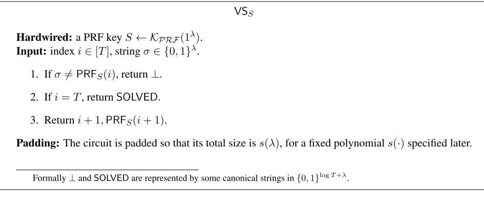
The core of the hard SVL distribution produced by I will be an obfuscatedverify and sign circuit that given a valid signature on an indexiproduces a signature on the next indexi+ 1, where signatures will be implemented by the puncturable PRF. The circuit is formally described in Figure 1.

VSS

Hardwired:a PRF keyS← KPRF(1λ).

Input:indexi∈[T], stringσ∈ {0,1}λ_.

1. Ifσ6=PRFS(i), return⊥.

2. Ifi=T, returnSOLVED.

3. Returni+ 1,PRFS(i+ 1).

Padding:The circuit is padded so that its total size iss(λ), for a fixed polynomials(·)specified later.

Formally⊥andSOLVEDare represented by some canonical strings in{0,1}logT+λ

.

Figure 1: The circuitVSS.

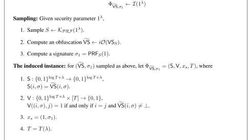
5.3 The Hard SVL Distribution

A random instance Φ

f

VS,σ1 ← I(1

λ₎ _{is associated with a (random) obfuscation}

f

VS of a verify-and-sign circuit (with respect to a random PRF seed) and a signatureσ1 on1 ∈ [T]. This induces a SVL instance

(S,V, xs, T) where the successor circuit ScomputesVSf, the verification circuit Vuses VSf to test inputs along the chain from the source inputxs = (1, σ1) to the target input (T, σT). The SVL distribution is

(13)

Φ

f

VS,σ1 ← I(1

λ₎

Sampling:Given security parameter1λ,

1. SampleS← KPRF(1λ).

2. Compute an obfuscationVSf ←iO(VS_S).

3. Compute a signatureσ1=PRFS(1).

The induced instance:for(VSf, σ₁)sampled as above, letΦ f

VS,σ1 = (S,V, xs, T), where

1. S:{0,1}logT+λ _{→ {}₀_,₁_}logT+λ_,

S(i, σ) =VSf(i, σ).

2. V:{0,1}logT+λ_×_[_T_]_{→ {}₀_,₁_}_,

V((i, σ), j) = 1if and only ifi=jandVSf(i, σ)6=⊥.

3. xs= (1, σ1).

4. T =T(λ).

Figure 2: Sampling the hard SVL distribution.

I is an SVL sampler. To show that I indeed samples SVL instances (S,V, xs, T) according to

Defi-nition 2.2, we only need to check that, for i ∈ [T]and x ∈ {0,1}logT+λ_, _V₍_{x, i}_{) = 1} _{if and only if}

x=Si−1(xs); the rest of the requirements are purely syntactic and are satisfied by the way we have defined

our sampler. To see that the verification requirement is satisfied, note that by the definition ofVSS,S, V,

andxsit holds thatSi−1(xs) =VSi_S−1(1, σ1) = (i,PRFS(i)), andV((j, σ), i) = 1if and only ifj =iand

VS(j, σ)6=⊥, implying that(j, σ) = (i,PRFS(i)).

5.4 Hardness

We now show thatIsamples hard SVL instances; namely instances(S,V, xs, T)for which circuits of some

sub-exponential-size cannot find the targetxT =ST−1(xs). We prove the following proposition. Proposition 5.1. For anyAof size2O(λε

2

)_{and every}_λ_∈ N,

Pr



PRF_S(T)← A(VSf, σ₁)

S ← KPRF(1λ) f

VS←iO(VSS)

σ1←PRFS(1)



≤2−Ω(λ

ε2₎

.

(14)

[u, T](for every possible signature), meaning in particular thatA(VSf, σ₁)cannot find an accepting signature

σ∗forT. The second inputσ1 remainsPRFS(1)throughout all hybrids.

Hyb₁:The original experiment, whereVSf is aniOofVS_S =VS(1)_S .

Hyb₂: Here VSf is an iO of a circuitVS (2)

v,S,K0. The circuit has a random one-way function image v =

OWFK0(u), and on any input(i, σ), it returns⊥if OWF_K0(i) = v. The circuit is formally described in Figure 3.

VS(2)_v,S,K0

Hardwired: a PRF keyS ← KPRF(1λ), an injective OWF keyK0 ← KOWF(1λ 0

)forλ0 = logT, an imagev=OWFK0(u), foru←[T].

1. IfOWFK0(i) =v, return⊥.

Figure 3: The circuitVS(2)_v,S,K0.

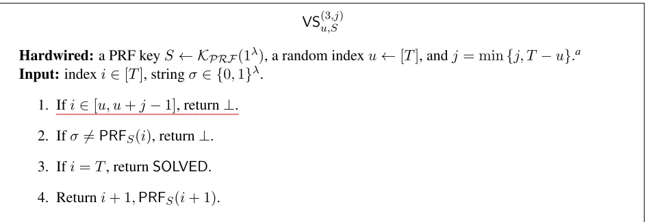
Hyb₃_,j, j ∈ [T + 1]: HereVSf is aniOof a circuitVS (3,j)

u,S . The circuit has a random indexu, and on any

input(i, σ), it returns⊥ifi∈[u, u+j]. The circuit is formally described in Figure 4.

VS(3_u,S,j)

Hardwired:a PRF keyS← KPRF(1λ), a random indexu←[T], andj= min{j, T−u}.a

1. Ifi∈[u, u+j−1], return⊥.

a

This is a convenient abuse of notation, which should be interpreted as “ifj > T−u, truncate it”.

(15)

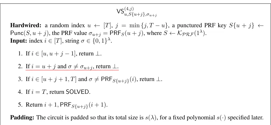
Hyb₄_,j, j ∈ [T]: HereVSf is an iO of a circuitVS (4,j)

u,S{u+j},σu+j. The circuit is the same asVS

(3,j)

u,S , only

that it has a punctured PRF keyS{u+j}, and the valueσu+j =PRFS(u+j)is hardwired. The circuit is

formally described in Figure 5.

VS(4_u,S,j_{)_u₊_j_}_,σu +j

Hardwired: a random index u ← [T], j = min{j, T −u}, a punctured PRF key S{u+j} ← Punc(S, u+j), the PRF valueσu+j =PRFS(u+j), whereS← KPRF(1λ).

2. Ifi=u+jandσ6=σu+j, return⊥.

3. Ifi∈[u+j+ 1, T]andσ =6 PRF_S{u+j}(i), return⊥. 4. Ifi=T, returnSOLVED.

5. Returni+ 1,PRFS{u+j}(i+ 1).

Figure 5: The circuitVS(4_u,S,j_{)_u₊_j_}_,σu +j.

Hyb₅_,j, j ∈[T]: HereVSf is an iO of a circuitVS (5,j)

u,S{u+j},σu+j. The circuit is the same asVS

(4,j)

u,S{u+j},σu+j,

only that the hardwiredσu+j is not set toPRFS(u+j), but sampled uniformly at random from{0,1}λ,

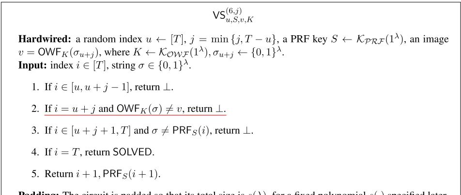
Hyb₆_,j, j ∈[T]: HereVSf is an iO of a circuitVS (6,j)

u,S,v,K. The circuit is the same asVS

(5,j)

u,S{u+j},σu+j, only

that instead of storingσu+j in the clearv=OWFK(σu+j)is stored, and comparison ofσandσu+jis done

by comparingOWFK(σ)andOWFK(σu+j). HereKis a key for an injective OWF from the familyOWF.

(16)

VS(6_u,S,v,K,j)

Hardwired: a random indexu ← [T], j = min{j, T−u}, a PRF keyS ← KPRF(1λ), an image

v=OWFK(σu+j), whereK← KOWF(1λ), σu+j ← {0,1}λ. Input:indexi∈[T], stringσ∈ {0,1}λ_.

2. Ifi=u+jandOWFK(σ)6=v, return⊥.

3. Ifi∈[u+j+ 1, T]andσ 6=PRFS(i), return⊥.

Figure 6: The circuitVS(6_u,S,v,K,j) .

The padding parameters(λ). We chooses(λ) so that each of the circuitsVSf ···

···considered above can be implemented by a circuit of size at mosts(λ)/3. (The extra1/3slack is taken to satisfy Lemma 5.1 in the analysis below.)

We prove the following:

Claim 5.1. For any2O(λε2)-size distinguisherD, allλ∈_N, and allj∈[T]:

1. |Pr[D(Hyb₁) = 1]−Pr[D(Hyb₂) = 1]| ≤2−Ω(λε

2 )_,

2. Pr[D(Hyb₂) = 1]−Pr[D(Hyb₃_,₁) = 1]

≤2−Ω(λ

ε₎

,

3. Pr[D(Hyb₃_,j) = 1]−Pr[D(Hyb₄_,j) = 1]

≤2−Ω(λ

ε₎

,

4. Pr[D(Hyb₄_,j) = 1]−Pr[D(Hyb₅_,j) = 1]

≤2−Ω(λ

ε₎

,

5. Pr[D(Hyb₅_,j) = 1]−Pr[D(Hyb₆_,j) = 1]

≤2−Ω(λ

ε₎

,

6. Pr[D(Hyb₆_,j) = 1]−Pr[D(Hyb₃_,j₊₁) = 1]

≤2−Ω(λ

ε₎

,

where the view ofDin each hybrid consists of the corresponding obfuscatedVSf andσ₁=PRF_S(1).

Proving the above claim will conclude the proof of Proposition 5.1 since it implies that

Pr

"

σ ← A(VSf, σ₁)

f

VS(T, σ)6=⊥

f

VS←iO(VSS)

#

≤

Pr

"

σ← A(VSf, σ₁)

f

VS(T, σ)6=⊥

f

VS←iO(VS(3_S,u,T+1))

#

+ 2−Ω(λε

2

) ₊_T_·₂−Ω(λε₎

=

0 + 2−Ω(λε

2

) ₊₂λε/2

·2−Ω(λε)= 2−Ω(λε

(17)

where the first to last equality follows from the fact thatVS(3_S,u,T+1)(T, σ) =⊥for anyσ.

Proof of Claim 5.1. We now prove each of the items in the claim.

Proof of 1 and 6.Recall that here we need to show that

1. |Pr[D(Hyb₁) = 1]−Pr[D(Hyb₂) = 1]| ≤2−Ω(λε2)_,

6. Pr[D(Hyb₆_,j) = 1]−Pr[D(Hyb₃_,j₊₁) = 1]

≤2−Ω(λ

ε₎

.

In both cases, one obfuscated program differs from the other on exactly a single point, which is the unique (random) preimage of the corresponding image v (in the first case v = OWFK0(u), and in the second

v=OWFK(σu+j)).

To prove the claim, we rely on a lemma proven in [BCP14] that roughly shows that, for circuits that only differ on a single input, iO implies what is known asdiffering input obfuscation[BGI+01], where it is possible to efficiently extract from any iO distinguisher an input on which the underlying circuits differ.

Lemma 5.1(special case of [BCP14]). LetiObe a(t, δ)-secure indistinguishability obfuscator for P/poly. There exists a PPT oracle-aided extractor E, such that for anytO(1)-size distinguisherD, and two equal size circuitsC0, C1differing on exactly one inputx∗, the following holds. LetC00, C10 be padded versions of

C0, C1of sizes≥3· |C0|.

If |Pr[D(iO(C₀0) = 1]−Pr[D(iO(C₁0) = 1]|=η≥δ(s)o(1) ,

then Pr

h

x∗ ← ED(·)(11/η, C0, C1) i

≥1−2−Ω(s) .

Using the lemma, we show that if either item 1 or 6 do not hold, we can invoke the distinguisher Dto invert the underlying one-way function. The argument is similar in both cases up to different parameters; for concreteness, we focus on the first. Assume that for infinitely many λ ∈ _N, D distinguishes Hyb₁

fromHyb₂ with gap η(λ) = 2−o(λε

2

)_{. Then, by averaging, with probability}_η₍_λ₎_/₂ _{over the choice of}

u, K0,Ddistinguishes the two distributions conditioned on these choices with gap η(λ)/2. Thus, we can invoke the extractorE given by Lemma 5.1 to invert the one-way function familyOWF with probability

η(λ) 2 ·(1−2

−Ω(λ)₎_≥₂−o(λε2)_{in time}_t

E(λ)·tD(λ)≤η(λ)−O(1)·2O(ε

2₎

= 2O(λε2)_{. Note that, indeed, given}

the image and the one-way function key, the inverter can construct the corresponding circuits efficiently. Recall thatOWF0_K is defined on inputs of sizeλ0 = logT =λε/2, and is(2−λ0ε,2λ0ε)-secure. Thus we get a contradiction to its one-wayness.

Proof of 2.Recall that here we need to show that

2. Pr[D(Hyb₂) = 1]−Pr[D(Hyb₃_,₁) = 1]

≤2−Ω(λ

ε₎

.

Here the two obfuscated programs compute the exact same function. Specifically, a comparison in the clear of two valuesianduis replaced by comparison of their corresponding values under an injective one-way function. Thus, the required indistinguishability follows from theiO(2λε,2−λε)-security.

3. Pr[D(Hyb₃_,j) = 1]−Pr[D(Hyb₄_,j) = 1]

≤2−Ω(λ

ε₎

.

(18)

any other index, the punctured keyS{u+j} is used. Thus, by the functionality guarantee of puncturing the two functions are the same, and indistinguishability follows from iO.

3. Pr[D(Hyb₄_,j) = 1]−Pr[D(Hyb₅_,j) = 1]

≤2−Ω(λ

ε₎

.

The only difference between the two obfuscated circuit distributions is that in the first the hardwired value

σu+j is PRFS(u+j), whereas in the second it is sampled independently uniformly at random.

Indistin-guishability follows from the(2λε,2−λε)-pseudo-randomness at the punctured point guarantee. Note that, indeed, given punctured keyS{u+j}andσu+j, a distinguisher can construct the corresponding circuits

efficiently.

5. Pr[D(Hyb₅_,j) = 1]−Pr[D(Hyb₆_,j) = 1]

≤2−Ω(λ

ε₎

.

Here also, the two obfuscated programs compute the exact same function. First, the comparison ofσ and

σu+jis replaced by comparison of their corresponding values under an injective one-way function. In

addi-tion, the punctured keyS{u+j}is replaced with a non-punctured keyS. This does not affect functionality as the two keys compute the same function on all points exceptu+j, and the circuits in the two hybrids treat any inputu+j, σ, independently of the PRF key. Thus, indistinguishability follows from iO.

This concludes the proof of the Claim 5.1 and Proposition 5.1.

5.5 Hardness Tradeoffs

In the hard SVL distribution constructed above, we assumed all cryptographic primitives are sub-exponentially hard. We now explain how this can be relaxed, and what are the tradeoffs between the hardness of the dif-ferent primitives (and the SVL hardness itself). Letf(·), g(·), h(·)be sub-linear functions and assume that

OWFis(2f(λ),2−f(λ))-secure,PRF is(2g(λ),2−g(λ))-secure, andiOis(2−h(λ),2−h(λ))-secure. We can restate Claim 5.1 as follows.

Claim 5.2 (Claim 5.1 generalized). For any distinguisher D of size at most 2O(m(λ)) where m(λ) = min(f(λ), g(λ), h(λ)), allλ∈_N, and allj∈[T]:

1. |Pr[D(Hyb₁) = 1]−Pr[D(Hyb₂) = 1]| ≤2−Ω(f(logT))+ 2−Ω(h(λ)), 2. Pr[D(Hyb₂) = 1]−Pr[D(Hyb₃_,₁) = 1]

≤2−Ω(h(λ)),

3. Pr[D(Hyb₃_,j) = 1]−Pr[D(Hyb₄_,j) = 1]

≤2−Ω(h(λ)),

4. Pr[D(Hyb₄_,j) = 1]−Pr[D(Hyb₅_,j) = 1]

≤2−Ω(g(λ)),

5. Pr[D(Hyb₅_,j) = 1]−Pr[D(Hyb₆_,j) = 1]

≤2−Ω(h(λ)),

6. Pr[D(Hyb₆_,j) = 1]−Pr[D(Hyb₃_,j₊₁) = 1]

(19)

The overall probability of solving the SVL can be then bounded by

2−Ω(f(logT))+T·(2−Ω(f(λ))+ 2−Ω(g(λ))+ 2−Ω(h(λ))) .

In particular, form(·)defined as above, we can guarantee(2m(λ),2−m(λ))-hardness of SVL as long as 1. m(λ) =ω(log(T) + logm(λ)).

2. f(logT) =ω(logm(λ)).

For instance, for any constantε <1, we can set

• T = 2(logλ)2/ε_,

• f(λ) =λε(OWF is still sub-exponential),

• g(λ) =h(λ) = (logλ)2+2/ε(PRF andiOare qausipolynomial).

Alternatively, we can set

• T = 22(logλ)

ε

,

• f(λ) =g(λ) =h(λ) = 2(logλ)

1+ε

2

(all primitives are only2λo(1)-secure).

Can we rely only on polynomial hardness? We do not know how to show SVL hardness based only on polynomially secure primitives. In particular, with the approach described aboveOWF cannot be quasi-polynomially (let alone quasi-polynomially) secure, sincef(f(λ)) = ω(logm(λ)) = ω(logf(λ)). In addition,

T(λ)cannot be polynomial as long as we aim to deal with distinguishers of arbitrary polysizeλO(1), which in turn implies thatPRF andiOcannot be polynomially secure.

We could, however, relaxiO,PRF to be polynomially secure if we assumeOWF is exponentially-secure; concretely, thatOWF cannot be inverted with probability greater than2−ελ in time less than 2ελ for some constantε < 1. Moreover, doing so we need to settle for worst-case hardness of SVL, rather than average-case as above. Specifically, rather than considering SVL instances with respect to one fixed functionT(λ), we can consider SVL instances with respect to everyT(λ) ∈

λ, λ2, . . . , λlogλ . In the resulting distribution, for anyλc-size circuit family, there exists a sequence of instances (or distributions on instances) on which it fails; these are the instances withT λc0·c/ε, wherec0is a constant that depends on polynomial overhead of the extractor given by Lemma 5.1.

Acknowledgements

(20)

References

[AB15] Benny Applebaum and Zvika Brakerski. Obfuscating circuits via composite-order graded en-coding. InTCC, 2015.

[AJ15] Prabhanjan Ananth and Abhishek Jain. Indistinguishability obfuscation from compact func-tional encryption. InCrypto, 2015.

[AKV04] Tim Abbot, Daniel Kane, and Paul Valiant. On algorithms for nash equilibria. Unpublished manuscript. http://web.mit.edu/tabbott/Public/final.pdf, 2004.

[BCC+14] Nir Bitansky, Ran Canetti, Henry Cohn, Shafi Goldwasser, Yael Tauman Kalai, Omer Paneth, and Alon Rosen. The impossibility of obfuscation with auxiliary input or a universal simula-tor. InAdvances in Cryptology - CRYPTO 2014 - 34th Annual Cryptology Conference, Santa Barbara, CA, USA, August 17-21, 2014, Proceedings, Part II, pages 71–89, 2014.

[BCP14] Elette Boyle, Kai-Min Chung, and Rafael Pass. On extractability obfuscation. InTCC, pages 52–73, 2014.

[Ben89] Charles H. Bennett. Time/space trade-offs for reversible computation. SIAM J. Comput., 18(4):766–776, 1989.

[BGI+01] Boaz Barak, Oded Goldreich, Russell Impagliazzo, Steven Rudich, Amit Sahai, Salil P. Vadhan, and Ke Yang. On the (im)possibility of obfuscating programs. InCRYPTO, pages 1–18, 2001.

[BGI14] Elette Boyle, Shafi Goldwasser, and Ioana Ivan. Functional signatures and pseudorandom functions. InPublic Key Cryptography, pages 501–519, 2014.

[BGK+14] Boaz Barak, Sanjam Garg, Yael Tauman Kalai, Omer Paneth, and Amit Sahai. Protecting obfuscation against algebraic attacks. InAdvances in Cryptology - EUROCRYPT 2014 - 33rd Annual International Conference on the Theory and Applications of Cryptographic Techniques, Copenhagen, Denmark, May 11-15, 2014. Proceedings, pages 221–238, 2014.

[BPW15] Nir Bitansky, Omer Paneth, and Daniel Wichs. Perfect structure on the edge of chaos. IACR Cryptology ePrint Archive, 2015:126, 2015.

[BR14] Zvika Brakerski and Guy N. Rothblum. Virtual black-box obfuscation for all circuits via generic graded encoding. In Theory of Cryptography - 11th Theory of Cryptography Con-ference, TCC 2014, San Diego, CA, USA, February 24-26, 2014. Proceedings, pages 1–25, 2014.

[BV15] Nir Bitansky and Vinod Vaikuntanathan. Indistinguishability obfuscation from functional en-cryption. InFOCS, 2015.

[BW13] Dan Boneh and Brent Waters. Constrained pseudorandom functions and their applications. In

ASIACRYPT (2), pages 280–300, 2013.

(21)

[CDT09] Xi Chen, Xiaotie Deng, and Shang-Hua Teng. Settling the complexity of computing two-player nash equilibria. J. ACM, 56(3), 2009.

[DGP09] Constantinos Daskalakis, Paul W. Goldberg, and Christos H. Papadimitriou. The complexity of computing a nash equilibrium. SIAM J. Comput., 39(1):195–259, 2009.

[GGH+13] Sanjam Garg, Craig Gentry, Shai Halevi, Mariana Raykova, Amit Sahai, and Brent Waters. Candidate indistinguishability obfuscation and functional encryption for all circuits. InFOCS, 2013.

[GGM86] Oded Goldreich, Shafi Goldwasser, and Silvio Micali. How to construct random functions. J. ACM, 33(4):792–807, 1986.

[GK05] Shafi Goldwasser and Yael Tauman Kalai. On the impossibility of obfuscation with auxiliary input. InFOCS, pages 553–562, 2005.

[GLSW14] Craig Gentry, Allison B. Lewko, Amit Sahai, and Brent Waters. Indistinguishability obfusca-tion from the multilinear subgroup eliminaobfusca-tion assumpobfusca-tion. IACR Cryptology ePrint Archive, 2014:309, 2014.

[Gol11] Paul W. Goldberg. A survey of ppad-completeness for computing nash equilibria. CoRR, abs/1103.2709, 2011.

[HPV89] Michael D. Hirsch, Christos H. Papadimitriou, and Stephen A. Vavasis. Exponential lower bounds for finding brouwer fix points. J. Complexity, 5(4):379–416, 1989.

[Jac91] A hierarchically constrained kinetic ising model. Zeitschrift fr Physik B Condensed Matter, 84(1), 1991.

[Jeˇr] Emil Jeˇr´abek. Integer factoring and modular square roots. Journal of Computer and System Sciences. Accepted.

[KMN+14] Ilan Komargodski, Tal Moran, Moni Naor, Rafael Pass, Alon Rosen, and Eylon Yogev. One-way functions and (im)perfect obfuscation. IACR Cryptology ePrint Archive, 2014:347, 2014.

[KPTZ13] Aggelos Kiayias, Stavros Papadopoulos, Nikos Triandopoulos, and Thomas Zacharias. Del-egatable pseudorandom functions and applications. In ACM Conference on Computer and Communications Security, pages 669–684, 2013.

[LR88] Michael Luby and Charles Rackoff. How to construct pseudorandom permutations from pseu-dorandom functions. SIAM J. Comput., 17(2):373–386, 1988.

[MP91] Nimrod Megiddo and Christos H. Papadimitriou. On total functions, existence theorems and computational complexity. Theor. Comput. Sci., 81(2):317–324, 1991.

[Nas51] John Nash. Non-cooperative Games. The Annals of Mathematics, 54(2):286–295, 1951.

(22)

[Pap94] Christos H. Papadimitriou. On the complexity of the parity argument and other inefficient proofs of existence. J. Comput. Syst. Sci., 48(3):498–532, 1994.

[PST14] Rafael Pass, Karn Seth, and Sidharth Telang. Indistinguishability obfuscation from semantically-secure multilinear encodings. InAdvances in Cryptology - CRYPTO 2014 - 34th Annual Cryptology Conference, Santa Barbara, CA, USA, August 17-21, 2014, Proceedings, Part I, pages 500–517, 2014.

[Rub14] Aviad Rubinstein. Inapproximability of nash equilibrium. CoRR, abs/1405.3322, 2014.

[SW14] Amit Sahai and Brent Waters. How to use indistinguishability obfuscation: Deniable encryp-tion, and more. InSTOC, 2014.

[Zim14] Joe Zimmerman. How to obfuscate programs directly. IACR Cryptology ePrint Archive, 2014:776, 2014.

A

Pseudo-code Descriptions of

S

j

and

P

j

Algorithm A.1The functionS1:

Input: Base stateub = (x, i)and the current nodeN = (u1, . . . , ut)

1: ifN contain an invalid statethen

2: return N unchanged{Not on path (Condition 1)}

3: end if

4: ifuj is freethen

5: Setu1←S(ub)

6: return (u1, . . . , ut)

7: else

8: return N unchanged{End of path or not on path (Condition 2)}

(23)

Algorithm A.2The functionSj forj >1:

3: end if

4: ifuj is freethen

5: N0 ←Sj−1(ub, N){First part}

6: ifN0 6=N then

7: return N0

8: else iffor allk∈[j−1],uk=v(i+ 2j−1−2k−1)then

9: Setuj ←S(u1){First part ended, first step of second part} 10: return (u1, . . . , ut)

11: end if

13: else ifuj =v(i+ 2j−1)then

14: iffor everyk∈[j−1],ukis either free oruk < uj then

15: N0 ←Pj−1(ub, N){Second part}

16: ifN06=N then

17: return N0

18: else iffor allk∈[j−1],ukis freethen

19: return Sj−1(uj, N){Second part ended, first step of third part}

20: end if

22: else iffor everyk∈[j−1],ukis either free oruk> uj then

23: return Sj−1(uj, N){Third part}

24: end if

25: end if

26: return N unchanged{Not on path (Conditions 2 and 3)}

Algorithm A.3The functionP1:

3: end if

4: ifuj =v(i+ 1)then

5: Setu1←v(1) 6: return (u1, . . . , ut)

7: else

8: return N unchanged{End of path or not on path (Condition 2)}

(24)

Algorithm A.4The functionPjforj >1:

3: end if

4: ifuj is freethen

5: return Pj−1(ub, N){Third part}

6: else ifuj =v(i+ 2j−1)then

7: iffor everyk∈[j−1],ukis either free oruk < uj then

8: N0 ←Sj−1(ub, N){Second part}

9: ifN06=N then

10: return N0

11: else iffor allk∈[j−1],uk =v(i+ 2j−1−2k−1)then

12: Setuj ←v(1){Second part ended, first step of third part}

13: return (u1, . . . , ut)

14: end if

16: else iffor everyk∈[j−1],ukis either free oruk> uj then

17: N0 ←Pj−1(uj, N){First part}

18: ifN06=N then

19: return N0

20: else iffor allk∈[j−1],ukis freethen

21: return Sj−1(ub, N){First part ended, first step of third part}

22: end if

23: end if

24: end if