The Deep Ocean Density Structure at the Last Glacial Maximum: What Was It and Why?

(1)

The deep ocean density structure at the Last Glacial

Maximum: What was it and why?

Thesis by

Madeline Diane Miller

In Partial Fulfillment of the Requirements for the Degree of

Doctor of Philosophy

California Institute of Technology Pasadena, California

2014

(2)

ii

c

2014

(3)

iii

into the sea all the rivers go, and yet the sea is never filled, and still to their goal the

rivers go

(4)

iv

Acknowledgements

The work described in this thesis would not have been possible without my advisor, Jess Adkins. He provided the impetus, and the structural and intellectual support for my projects. Further, Jess has encouraged me to explore bold research paths and, when setbacks inevitably arose, he helped me learn from them, in the process nudging me towards becoming an independent researcher. Jess models and teaches a broad, problem-based approach to research. While many oceanographers incorporate data or concepts outside their traditional focus (i.e. biological, physical, or chemical) to their work, Jess does not cross disciplinary boundaries, he simply does not see them. He teaches us both by telling us directly and, even more impressively, by his example that we should always use the best tool to answer our questions, whether the tool is something we already know or is well outside our “tool box”. I look forward to continuing to learn from Jess in the future.

I am indebted to Nadia Lapusta for her support as the Mechanical Engineering option representative in smoothing the way for me to pursue an unconventional thesis topic. My thesis committee – John Brady, Chris Charles, Richard Murray, and Mark Simons – have been equally open-minded in assisting with work outside their primary areas of interest and very generous with their time.

(5)

v

Over the last two years, Mark Simons has been slowly and stealthily saddled with the role of being my unofficial second advisor. Mark’s expertise and guidance were essential to the work in this thesis that relies on inverse methods, and he has shared liberally his time, ideas, code, server, and scientific contacts. I continue to be impressed by Mark’s tireless enthusiasm for science and his ability to see the construction hidden behind every research roadblock, best encapsulated by his own words: “...but look how much you’ve

learned!”

Sarah Minson has not only generously allowed me to use her code, CATMIP, but has also provided significant technical support in applying CATMIP to my research problems, despite the fact they do not overlap with hers. Sarah has additionally shared with me a great deal of her time and expertise on Bayesian MCMC parameter estimation.

Through Mark’s and Sarah’s introductions, my work has been improved from conversa-tions with Francisco Ortega, Bryan Riel, Michael Aivazis and Jim Beck.

I have been lucky to share many hours in the last few years with the vibrant people in my research group: Anna Beck, Andrea Burke, Stacy Carolin, Alex Gagnon, Sophie Hines, Paige Logan, Nele Meckler, Guillaume Paris, Ted Present, James Rae, Morgan Raven, Alex Rider, Harald Sodemann, Adam Subhas, and Nithya Thiagarajan. I have learned many things from all of you, not the least of which is how to keep the fun in good science.

(6)

vi

The NASA Advanced Supercomputer (NAS) support and Caltech’s GPS IT and High Per-formance Computing (HPC) support, particularly Mike Black and Naveed Near-Ansari, have been extremely responsive and patient in assisting me debug issues on Pleiades, Salacia and Fram over the course of my research. I am particularly grateful that experts in the NAS Control Room are available 24x7.

At various stages in building experiments at Caltech, some of which are not discussed in this thesis, I have benefited greatly from the help of all of the machinists in the Physics shop, as well as Caltech’s scientific glassblower Rick Gerhart.

(7)

vii

Abstract

The search for reliable proxies of past deep ocean temperature and salinity has proved difficult, thereby limiting our ability to understand the coupling of ocean circulation and climate over glacial-interglacial timescales. Previous inferences of deep ocean temperature and salinity from sediment pore fluid oxygen isotopes and chlorinity indicate that the deep ocean density structure at the Last Glacial Maximum (LGM,_∼20,000 years BP) was set by salinity, and that the density contrast between northern and southern sourced deep waters was markedly greater than in the modern ocean. High density stratification could help explain the marked contrast in carbon isotope distribution recorded in the LGM ocean relative to that we observe today, but what made the ocean’s density structure so different at the LGM? How did it evolve from one state to another? Further, given the sparsity of the LGM temperature and salinity data set, what else can we learn by increasing the spatial density of proxy records?

(8)

viii

(9)

ix

Contents

Acknowledgements iv

Abstract vii

Contents ix

List of Figures xiii

List of Tables xxvii

1 Introduction 1

2 Reconstructingδ18O and salinity histories from pore fluid profiles: What

can we learn from regularized least squares? 12

2.1 Introduction . . . 12

2.2 Methods . . . 17

2.2.1 The forward problem . . . 17

2.2.1.1 Simplifying assumptions . . . 17

2.2.1.2 Finite difference solution technique . . . 20

2.2.1.3 Green’s function approach . . . 20

2.2.2 The inverse problem . . . 21

2.2.2.1 Ill-posed nature of inverse problem . . . 21

2.2.2.2 Truncated SVD solution . . . 23

2.2.2.3 Zeroth-order Tikhonov regularization . . . 24

2.2.2.4 Second-order Tikhonov regularization . . . 26

(10)

x

2.3 Results . . . 29

2.3.1 Recovering a stretched sea level boundary condition . . . 29

2.3.1.1 Properties of G . . . 30

2.3.1.2 TSVD least squares inverse solution . . . 30

2.3.1.3 Zeroth order Tikhonov regularization . . . 33

2.3.1.4 Zeroth order Tikhonov regularization with noise . . . 34

2.3.1.5 Resolution of the inverse solution . . . 42

2.3.1.6 Second order Tikhonov regularization . . . 46

2.3.1.7 Variable damping . . . 53

2.3.2 The effect of the diffusion parameter . . . 56

2.4 Discussion . . . 61

2.5 Conclusions . . . 63

3 What is the information content of pore fluid δ18_{O and [Cl}−_]? ₆₄ 3.1 Introduction . . . 64

3.2 Methods . . . 68

3.2.1 Forward model . . . 68

3.2.2 The inverse problem . . . 70

3.2.2.1 Bayesian Markov Chain Monte Carlo sampling . . . 70

3.2.2.2 Model parameterization . . . 71

3.2.2.3 Cost function . . . 72

3.2.3 Choice of priors . . . 72

3.2.3.1 Prior information from sea level records . . . 73

3.2.3.2 Prior information from modern ocean property spreads . . 74

3.2.3.3 Accounting for different-than-modern past ocean property spreads . . . 77

3.2.3.4 Diffusion coefficient prior . . . 78

3.3 Results . . . 79

3.3.1 Synthetic problem . . . 79

3.3.1.1 Linear problem – uninformative prior . . . 80

(11)

xi

3.3.1.3 Linear Problem – recovery of models with known variance

and covariance . . . 99

3.3.1.4 Nonlinear problem – recovery of models with known vari-ance and covarivari-ance, allowing D0 and initial condition to vary . . . 114

3.3.2 Real data . . . 119

3.4 Discussion and ongoing investigations . . . 121

4 New techniques for sediment interstitial water sampling 147 4.1 Motivation and background . . . 147

4.2 Methods . . . 150

4.2.1 Shipboard sampling . . . 150

4.2.1.1 Squeeze samples . . . 150

4.2.1.2 Rhizon samples . . . 151

4.2.2 δ18_{O and} _δ_{D measurements} _{. . . 153}

4.2.3 [Cl−] measurements . . . 154

4.3 Results . . . 156

4.3.1 Stable isotopes . . . 157

4.3.2 Chloride . . . 158

4.4 Discussion . . . 160

5 The role of ocean cooling in setting glacial southern source bottom water salinity 167 Abstract 168 5.1 Introduction . . . 169

5.2 Methods . . . 173

5.2.1 Model Setup . . . 173

5.2.2 Salinity Tracers . . . 176

5.2.3 Boundary Conditions . . . 177

(12)

xii

5.2.5 Experiments . . . 181

5.3 Results and Discussion . . . 182

5.3.1 Diagnosis of Water Mass Changes – Net Salinity Fluxes and Changes184

5.3.2 Diagnosis of Water Mass Changes – Regional Variations and

Salin-ity Flux Tracers . . . 188

5.3.3 Diagnosis of Water Mass Changes – Regional Differences in Ice Shelves195

5.3.4 Relevance to Glacial Oceans . . . 197

5.3.5 The Effect of Unmodelled Processes . . . 198

6 Concluding remarks 202

A Titration methods for [Cl−] measurement 206

A.1 Theory . . . 206

A.2 Equipment. . . 207

A.3 Standards . . . 208

(13)

xiii

List of Figures

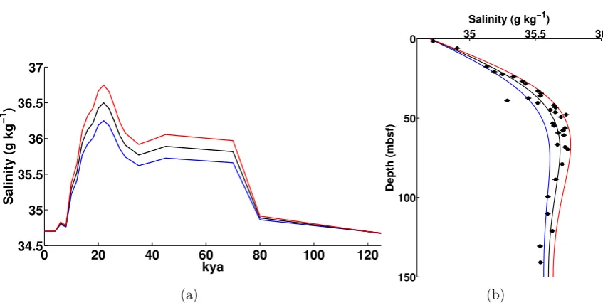
2.1 Illustration of the method previously used to reconstruct the LGM salinity

and δ18_{O. Changes in salinity scaled to the sea level curve, up to a scaling}

constant. Low sea level corresponds to high salinity and vice versa. (a)

shows boundary conditions produced using three different scaling factors,

and (b) shows the model output using those boundary conditions overlaid on

measured data in sediment pore fluids (black circles). Each color corresponds

to a different LGM – modern scaling factor. . . 15

2.2 Picard plot for G size 251 x 251. . . 31

2.3 (a) shows the synthetic model (red) used to generate synthetic data and the model recovered using the TSVD method (blue). (b) is the synthetic data (red) generated by the synthetic model and used to find the inverse solution plotted against the data generated by the recovered model using TSVD (blue). 32 2.4 L-curve for G size 251 x 251, 0th order Tikhonov regularization . . . 33

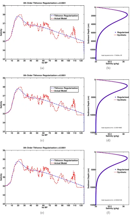
2.5 0th order Tikhonov regularization, no noise . . . 36

2.8 0th order Tikhonov regularization with noise,G 251 x251 . . . 39

2.9 0th order Tikhonov regularization with noise,G 301 x 626 . . . 40

2.10 0th order Tikhonov regularization with noise,G 301 x 1251 . . . 41

2.11 Resolution diagonals and LGM spike tests, 0th order regularization . . . 45

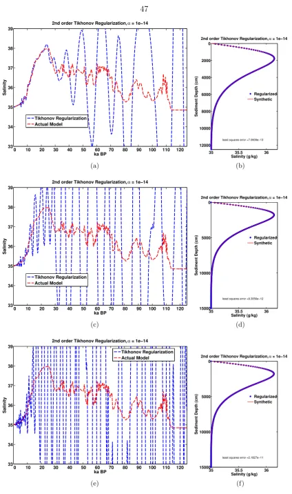
2.12 2nd order regularization, no noise, using L-curve criterion for α . . . 47

2.13 2nd order regularization, no noise, using L-curve criterion for α . . . 48

(14)

xiv

2.15 2nd order regularization with noise, α chosen with discrepancy principle,G

251 x 251 . . . 50

301 x 626 . . . 51

301 x 1251 . . . 52

2.18 2nd order resolution matrix diagonals and LGM spike test, G 251 x 251 . . 53

2.19 Spike tests comparing the skill of constant vs. variable damping through the

sensitivity matrix technique. The first row, (a) - (c) use a constant damping

parameter α = 1 and the standard second-order Tikhonov regularization.

The second row, (d) - (f) use α=1 and the variable sensitivity matrix S in

place of the uniform L.. . . 55

2.21 D0 = 2.9×10−5 cm2 s−1, 2nd order regularization with noise, G251 x 251 . 58

2.22 0th order reg, D0 = 2.9× 10−7 cm2 s−1 (a) 0.05% noise G 251x251 and

discrep criterion (c) 0.1% noise (e) 0.5% noise (g) 1% noise. . . 59

2.23 2nd order reg, D0 = 2.9×10−7 cm2 s−1 (a) 0.05% noise G 251x251 and

discrep criterion (c) 0.1% noise (e) 0.5% noise (g) 1% noise. . . 60

3.1 Measured profiles of (a)δ18_{O and (b) salinity (converted from the measured}

[Cl−] values). Note that the x-axis for ODP Site 1239 in (a) has a wider range

than the others. The values in all of the measured data profiles increase

towards a local maximum several tens of meters below the sea floor.. . . 65

3.2 Information in the measured δ18_{O and [Cl}−_{] (shown converted to equivalent}

salinity). Circles represent the modern sediment-water interface value, while

triangles are the maximum value measured in the pore fluids between 0 and

100 mbsf. . . 66

3.3 Locations of the ODP sites where we have pore fluid profile measurements

ofδ18O and [Cl−] overlain on the modern ocean bottom water salinity. Note

that the range of modern ocean bottom water salinity is quite narrow. . . . 67

3.4 Reconstructions of past sea level relative to present (black circles) and the

points we use for sea level in computing the prior mean salinity and δ18_O

(15)

xv

3.5 (a) Modern S below 2000m, GISS database accessed 9/12/2012, excluding

the Mediterranean Sea. Blue curve is Gaussian distribution with standard

deviation used for priors (b) modernδ18O below 2000m . . . 76

3.6 Prior probability for D0 is log-normal centered on 50×10−6 cm2 s−1, with

standard deviation of the logarithm equal to 1.5. . . 79

3.7 Synthetic example with 0.05% noise added to the data. Units for salinity on

the y-axis are g kg−1. Red dashed line is the synthetic (true) model used to

generate the data. The black dots represent mean positions of prior salinity

nodes. The blue triangles are the posterior mean salinity nodes. (a) has 0

covariance in the prior, (b) has T= 1000 years covariance timescale prior, (c)

T=2000 years, (d) T = 3000 years, (e) T= 4000 years, (f) T = 5000 years,

(g) T = 6000 years. . . 83

3.8 Histograms of synthetic solution assuming 100 g kg−1 variance. Blue is the

histogram of the prior samples, red is the histogram of the posterior samples.

(a) has a prior with no covariance while (b) has a prior covariance timescale

of 6000 years . . . 85

3.9 Ratio of posterior variance to prior variance for the linear synthetic case with

100 = σ2

I and µI set by scaling to sea level curve. Each colored line depicts

a different value for the prior covariance timescale T, from 0 to 6000 years . 86

3.10 Posterior correlation maps for examples inverting the stretched sea level

curve using a wide (σ = 10 g kg−1) Gaussian prior with varying values of

T. The axes’ values are the age in ka BP of each node. Each colored block

is the posterior correlation between the nodes represented by the values

on the x and y axis. For this reason the maps are symmetric about the

diagonal. The scale is from -1 to 1 in unitless Pearson correlation coefficient

rx,y = E[(X

−µx)(Y−µy)]

σxσy . Values between -0.2 and 0.2 have been masked with white. (a) has 0 covariance in the prior, (b) has T= 1000 years covariance

timescale prior, (c) T=2000 years, (d) T = 3000 years, (e) T= 4000 years,

(16)

xvi

3.11 Shift in the mean solution from prior to posterior as a function of covariance

timescale T. Each line represents a different value of T in years, from 0 years

to 6000 years. As T increases, the temporal dependence of the mean shift is

flattened or damped. . . 88

3.12 Lomb-Scargle periodogram of the posterior mean for the stretched sea level

example using a wide Gaussian prior. The black line is the periodogram

of the prior mean for comparision. Each color is the periodogram of the

posterior mean with a different prior covariance timescale T in years, from 0

to 6000 years. The vertical lines overlain show the peak frequencies for the

prior and those of the posterior for the example T = 6000 years. . . 89

3.13 Synthetic example with 0.05% noise added to the data. The prior nodes

are independent (no covariance) Gaussians centered around a salinity curve

scaled to sea level with varying variance. (a) 0.02 g kg−1 (b) 0.5 g kg−1. (c)

1 g kg−1. Red dashed line is the synthetic (true) model used to generate the

data. The black dots represent mean positions of prior salinity nodes and

the black lines are the 10 highest probability samples from the prior. The

blue triangles are the posterior mean salinity nodes and the blue lines are

the 10 highest probability samples from the posterior. . . 93

3.14 Posterior correlation matrices for models shown in Fig. 3.13 where the prior

T=0. The axes’ values are the age in ka BP of each node. Each colored block

is the posterior correlation between the nodes represented by the values

rx,y = E[(X

−µx)(Y−µy)]

(17)

xvii

have Gaussian covariance with time scale T = 1000 years centered around

a salinity curve scaled to sea level with varying variance. (a) 0.02 g kg−1

(b) 0.5 g kg−1. (c) 1 g kg−1. Red dashed line is the synthetic (true) model

used to generate the data. The black dots represent mean positions of prior

salinity nodes and the black lines are the 10 highest probability samples from

the prior. The blue triangles are the posterior mean salinity nodes and the

blue lines are the 10 highest probability samples from the posterior. . . 94

3.16 Posterior correlation matrices for models shown in Fig. 3.15, where T =

1000 years. The axes’ values are the age in ka BP of each node. Each

colored block is the posterior correlation between the nodes represented by

the values on the x and y axis. For this reason the maps are symmetric

about the diagonal. The scale is from -1 to 1 in unitless Pearson correlation

coefficient rx,y = E[(X

−µx)(Y−µy)]

σxσy . Values between -0.2 and 0.2 have been masked with white. (a) 0.02 g kg−1 variance, (b) 0.5 g kg−1 variance, (c) 1

g kg−1 variance . . . 94

3.18 Posterior correlation matrices for models shown in Fig. 3.17 where T = 3000

years. The axes’ values are the age in ka BP of each node. Each colored

block is the posterior correlation between the nodes represented by the values

rx,y = E[(X

−µx)(Y−µy)]

(18)

xviii

3.20 Posterior correlation matrices for models shown in Fig. 3.19, where T=5000

years. The axes’ values are the age in ka BP of each node. Each colored

block is the posterior correlation between the nodes represented by the values

rx,y = E[(X

−µx)(Y−µy)]

σxσy . Values between -0.2 and 0.2 have been masked with white. (a) 0.02 g kg−1 variance, (b) 0.5 g kg−1 variance, (c) 1 g kg−1 variance 96

3.21 Histograms of synthetic solution assuming 0.02 g kg−1 variance. Blue is

the histogram of the prior samples, red is the histogram of the posterior

samples. (a) has a prior with no covariance while (b) has a prior covariance

timescale of 5000 years. Each box is one node of the time series we are

estimating. From left to right and top to bottom the nodes move forward in

time, starting at 125 ka BP and ending at the present, 0 ka BP. . . 100

3.22 Histograms of synthetic solution assuming 1 g kg−1 variance. Blue is the

histogram of the prior samples, red is the histogram of the posterior

sam-ples. (a) has a prior with 0 covariance while (b) has a prior with 5000 year

timescale covariance. Each box is one node of the time series we are

esti-mating. From left to right and top to bottom the nodes move forward in

(19)

xix

3.23 The ratio of posterior variance (σ2_F) to prior variance (σ2_I) for a range of

different input priors and data from the stretched sea level curve example.

Each color corresponds to a different value of T, the covariance timescale

in years, while each symbol is a different input variance. The symbols help

delineate the different lines, but the variance shrinkage is primarily a function

of T . . . 102

3.24 Shift in the mean of the posterior population (µF) with respect to the mean of

the prior distribution (µI), normalized to the mean of the prior distribution.

Each color corresponds to a different value of T, the covariance timescale in

years, while each symbol is a different input variance. . . 102

3.25 Difference between the posterior mean and the true synthetic model (g kg−1)

as a function of prior variance and covariance. Each color corresponds to

a different value of T, the covariance timescale in years. Each symbol is a

different input variance, from 0.02 to 1 g kg−1 . . . 103

3.26 Same as Figure 3.25, except also including the examples with wide Gaussian

prior σ2

I = 100 g kg

−1 _{. . . 103}

3.27 Ten random models drawn from the scaled sea level curve with variance 0.02

g kg−1 and covariance T = 4000 years. Red is the target or true model from

which the data was generated. Black circles are the mean of the posterior

samples. Black stars and dashed line are the mean priors . . . 105

3.28 Top: difference between the mean of the posterior and the true model (g

kg−1) used to generate the data for the 10 random sample synthetic models

shown in Figure 3.27, that were drawn from a distribution with 0.02 g kg−1

variance and 4000 year covariance timescale T. Bottom: difference between

the mean of the prior and the true model for the same set. . . 106

(20)

xx

variance and 0 year covariance timescale T. Bottom: difference between the

mean of the prior and the true model for the same set. . . 108

variance and 4000 year covariance timescale T. Bottom: difference between

the mean of the prior and the true model for the same set. . . 110

variance and 0 year covariance timescale T. Bottom: difference between the

mean of the prior and the true model for the same set. . . 112

3.35 Reduction in variance from (σ2

I) to posterior (σ2F) for random samples with

different variance and covariance drawn from known priors. Blue lines have

prior variance 0.02 g kg−1 while red lines have prior variance 0.5 g kg−1. The

reduction of variance from the prior to the posterior is a strong function of

covariance timescale T . . . 112

3.36 Reduction in variance from prior (σ2_I) to posterior (σ_F2) for random sample

models generated from a distribution with 0.02 g kg−1 =σ2 _{and 4000 years}

(21)

xxi

3.37 Reduction in variance from prior (σ2_I) to posterior (σ_F2) for random sample

models generated from a distribution with 0.02 g kg−1 =σ2 _{and 4000 years}

= T when CATMIP is fed the wrong prior (0.5 g kg−1 =σ_I2, 0 years = T) . 113

3.38 Reduction in variance from prior (σ2

I) to posterior (σF2) for random sample

models generated from a distribution with 0.02 g kg−1 =σ2 and 4000 years

= T when CATMIP is fed the wrong prior (0.02 g kg−1 =σ2

I, 0 years = T) 114

3.39 Top – difference between the true time series solution and the mean posterior,

compared to bottom – the difference between the prior and the true time

series solution for random synthetic model samples in the nonlinear problem

with 1=σ2_{, 0 years = T} _{. . . 115}

3.40 Top – difference between the true time series solution and the mean posterior,

compared to bottom – the difference between the prior and the true time

series solution for random synthetic model samples in the nonlinear problem

with 1=σ2_{, 6000 years = T} _{. . . 116}

3.41 Comparison of prior and posterior distributions of D0 for the nonlinear

ran-dom synthetic cases. (a) is a ranran-dom example from the distribution 0.05 g

kg−1=σ2, 0 years = T, (b) is a random example from the distribution 0.05 g

kg−1 =σ2_{, 6000 years = T, (c) is a random example from the distribution 1}

g kg−1 =σ2, 0 years = T, and (d) is a random example from the distribution

1 g kg−1 =σ2_{, 6000 years = T.} _{. . . 117}

3.42 Variance reduction in the posterior (σ_F2) relative to the prior (σ2_I) for random

synthetic cases drawn from the distribution 1 g kg−1=σ2_{, and both 0 and}

6000 years = T . . . 118

3.43 Comparison of prior (blue) and posterior (red) marginals for a random

syn-thetic drawn from the distribution 1=σ2, and both 0 years = T . . . 119

3.44 Mean of 1000 posteriorδ18_{O time series models recovered from data at sites}

ODP 981, 1063, 1093, 1123 and 1239, with varying prior assumptions (see

inset legends).. . . 122

3.45 Mean of 1000 posterior δ18O initial conditions recovered from data at sites

ODP 981, 1063, 1093, 1123 and 1239, compared to data (black stars), with

(22)

xxii

3.46 Mean of 1000 posterior D0 for δ18O recovered from data at sites ODP 981,

1063, 1093, 1123 and 1239, with varying prior assumptions (see inset legends).124

3.47 Mean of 1000 posterior salinity time series models recovered from data at

sites ODP 981, 1063, 1093, 1123 and 1239, with varying prior assumptions

(see inset legends). . . 125

3.48 Mean of 1000 posterior salinity initial conditions recovered from data at sites

ODP 981, 1063, 1093, 1123 and 1239, compared to data (black stars), with

varying prior assumptions (see inset legends). . . 126

3.49 Mean of 1000 posterior D0 for salinity recovered from data at sites ODP 981,

1063, 1093, 1123 and 1239, with varying prior assumptions (see inset legends).127

3.50 Marginal posterior distribution for D0 of δ18O at Site 981 with the prior

assumptions of σ2

I = 1 h and T = 2000 years.. . . 127

3.51 LGM value of (a) S and (b) δ18O . . . 129

3.52 T/S plots with LGM reconstructions usingσ2 _{= 1 for both}_δ18_{O and S (red)}

compared toAdkins et al.(2002) (blue) and modern (orange). Here we take

the LGM as the time with maximum in S. (a) uses a prior with T = 0 years

while (b) uses a prior with T = 6000 years . . . 130

3.53 T/S plots with LGM reconstructions usingσ2 _{= 0.05 for S and =0.1 for}_δ18_O

(red) compared to Adkins et al. (2002) (blue) and modern (orange). Here

we take the LGM as the time with maximum in S. (a) uses a prior with T

= 0 years while (b) uses a prior with T = 6000 years . . . 130

3.54 Modern mean annual salinity at ODP Sites 1123 and 1239 . . . 135

4.1 Intercomparison of measurements from Rhizon (black triangles) and squeeze

(open circles) samples as reported in Schrum et al. (2012). Note that the

reported error bars are smaller than the plot symbols. . . 149

4.2 Schematic of high-resolution sampling using syringes. Each numbered

sec-tion represents 1.5 m of core. CC denotes core catcher. The core barrel is

9.5 m long, but individual sediment cores vary in length. . . 151

4.3 Rhizon samplers in cores . . . 152

4.4 HR consistency standard. . . 156

(23)

xxiii

4.6 Depth profiles ofδ18O andδD measured in both squeeze and Rhizon samples

at site U1385 . . . 158

4.7 Histograms of offset between Rhizon measurements and squeeze sample

mea-surements interpolated to the Rhizon positions. (a)δ18_{O, (b)} _δ_D _{. . . 159}

4.8 Offset between Rhizon sample measurements and squeeze sample

measure-ments as a function of depth (mbsf). (a) δ18_{O, (b)}_δ_D _{. . . 159}

4.9 Depth profiles of [Cl−] measured in both squeeze and Rhizon samples at site

U1385 . . . 160

4.10 Histograms of the [Cl−] (g kg−1) offset between Rhizon sample measurements

and squeeze sample measurements interpolated to the depths of the Rhizon

samples . . . 161

4.11 [Cl−] (g kg−1) offset between Rhizon sample measurements and squeeze

sam-ple measurements as a function of depth . . . 161

4.12 Offset between Rhizon and squeeze sample [Cl−] as a function of the age of

the IAPSO standard (days) used to measure the Rhizon sample . . . 161

4.13 Hydrogen isotope ratios vs. oxygen isotope ratios . . . 164

4.14 Chloride fractionation vs. isotope ratios (a) shows chloride vs. δ18O, (b)

shows chloride vs. δD . . . 165

4.15 Fractionation vs. depth . . . 165

5.1 Histogram of modern Weddell Sea continental shelf properties (figure after

Nicholls et al. (2009)). See Table 1 for water mass abbreviations.

Continen-tal shelf in this figure is defined after Nicholls et al. (2009) as south of 70◦S

and west of 0◦. Curved lines are surface isopycnals separated by 0.1 kg m−3.

Gray scale shows the base 10 logarithm of the frequency of each value. Bin

(24)

xxiv

5.2 Computational domain and bathymetry. White area indicates floating ice

shelves and black area is land/grounded ice comprising the Antarctic

conti-nent. LIS: Larsen Ice Shelf, RIS: Ronne Ice Shelf, FIS: Filchner Ice Shelf.

We do not include ice shelves east of the Antarctic Peninsula. Model

do-main bathymetry in meters is represented by the gray scale. In the following

analyses we use the space between the ice shelf front and the 1000-m

con-tour as the continental shelf in order to include water in the Filchner and

Ronne depressions in our analysis. Note that water under the ice shelves is

not included, but the water found equatorward of the eastern Weddell ice

shelves is included. . . 174

5.3 Histogram of control integration continental shelf properties. Weddell Sea

continental shelf is defined after Nicholls et al. (2009) to be south of 70◦S

and west of 0◦. Gray scale shows the base 10 logarithm of the frequency of

each value. Bin sizes are 0.001 in both S and Θ0. . . 179

5.4 Θ0/S properties of water in two layers along domain bottom down to 1700

m from the control and from two sensitivity experiments at their annual

salinity maxima. Together these two layers represent, on average,_∼150 m of

vertical thickness. The open ocean and the shelf region west of the Antarctic

Peninsula are excluded. All potential temperatures are referenced to the

surface. Curved lines are isopycnals. The distance between the isopycnal

lines is 0.1 kg m−3 . . . 183

5.5 Sensitivity of volume-averaged domain salinity to volume-averaged domain

potential temperature. All values are 10-year averages. Each experiment is

(25)

xxv

5.6 Magnitude of salinity fluxes integrated over the entire domain. E–P–R =

evaporation ₋ precipitation ₋ runoff. For reference, 1010 _{g s}−1 _{= 6}_._{5 m}

yr−1 of sea ice exported (assuming a spatial cover of the total domain ocean

area), so the variation between the sea ice export between the control and

the coldest sensitivity experiment is _∼0.82–1.03 m yr−1. Precipitation and

runoff are prescribed in our experiments, so the change in E–P–R is due to

a change in evaporation only. The magnitude of the sea ice and evaporation

contributions to domain salinity are 0.5 – 1 order larger than the magnitude

of the ice shelf contribution in all experiments. However, the sea ice is much

less sensitive to ocean temperature change than the ice shelves. . . 186

5.7 Change in salinity fluxes integrated over the entire domain. Each experiment

is represented by the domain steady state volume-averaged potential

tem-perature. All values are 10-year averages. For reference, 109 g s−1 = 0.65 m

yr−1 of sea ice exported (assuming a spatial cover of the total domain ocean

area). Sea ice and evaporation are of approximately equal magnitude but

opposite sign; their combination is an order of magnitude smaller than all

other fluxes, that is, they essentially cancel each other’s contribution. . . . 187

5.8 Change in surface salinity fluxes over the continental shelf, computed as

sensitivity minus control experiment. Each experiment is represented on the

x-axis by the domain steady state volume average potential temperature.

All values are 10-year averages. The boundaries of the continental shelf are

taken as the 1000-meter depth contour, excluding land to the north and/or

west of the Antarctic Peninsula. For reference, 10−7 g s−1 is equivalent

to the export of 0.11 m yr−1 from the entire continental shelf. E–P–R =

evaporation ₋ precipitation ₋ runoff. The only change in E–P–R across

the experiments is due to evaporation. Salinity flux changes due to sea ice

(26)

xxvi

5.9 (a) Minimum sea ice area for three experiments, from left to right: η = 0,

η = 0.4, η = 0.8. (b) Maximum sea ice area for three experiments, from

left to right: η = 0, η = 0.4, η = 0.8. The color scale indicates grid cell

concentration and is unitless. All values represent a 10-year average and

a weekly average during the week in which the total sea ice volume is at

its yearly maximum. The 1000-m depth contour is overlain to indicate the

continental shelf break. Grounded ice is indicated by hash marks and floating

ice shelves are adjoined to the grounded ice and colored white. . . 190

5.10 Depth integrated salt tracer fields for the sensitivity experiment in which

the boundaries are cooled 40% towards the freezing point from the control

experiment (η = 0.4). Color values are in m g kg−1 and represent the

difference between the sensitivity and control experiments. All are 10-year

averages. Black shaded area is land, white shaded area is ice shelves and

the black contour line represents the location of the 1000-m bottom depth

contour. . . 193

5.11 Ice shelf and sea ice salinity tracer values integrated over the bottom

water-filled layer on the continental shelf. All values represent the 10-year-averaged

difference between sensitivity and control. The boundaries of the continental

shelf are taken as the area between the ice shelf front and the 1000-m depth

contour, shown in Fig. 5.2, excluding land to the north and/or west of the

Antarctic Peninsula. . . 194

5.12 Comparison of time-averaged and spatially-integrated volume melt rate of

ice shelves in western and eastern sectors of domain. The western sector

corresponds to the Filchner-Ronne Ice Shelf and all ice shelves in the

West-ern Weddell Sea. The eastWest-ern sector is all ice shelves to the east of the

Filchner-Ronne Ice Shelf. All values represent the 10-year-average of a

(27)

xxvii

List of Tables

2.1 Summary of G properties . . . 30

3.1 Sea level compilation . . . 137

(28)

1

Chapter 1

Introduction

Over the last _∼0.8 Ma (Ma = one million years), the Earth has experienced glacial cycles with a dominant _∼100 ka (ka = one thousand years) period (Ruddiman et al.,

1989, Lisiecki and Raymo, 2007). At the glacial maxima, ice sheets blanketed extensive

swaths of the northern hemisphere continents (CLIMAP Project Members,1976), and the mean annual atmospheric temperature dropped globally relative to temperatures during interglacials (glacial minima), with values of -2◦C over the tropics to -30◦C over the Northern Hemisphere continental ice sheets (Braconnot et al., 2007). While solar energy received by the Earth due to changes in the Earth’s orbit around the sun has major variability on periods of 23 ka, 41 ka and 100 ka, spectral analysis of temperature records in ocean sediments and ice cores over the last 0.8 million years shows that the magnitude of the 100 ka year climate variability is disproportionate to the changes in solar input on the same timescale. As compared to the solar forcing and climate response at 23 ka and 41 ka periods, the 100 ka climate cycle appears to be nonlinear with respect to solar variability. Thus, it is commonly believed that one or more process internal to the Earth’s climate system must explain the recent dominance of the 100 ka glacial cycle (Hays et al.,

1976,Imbrie et al., 1992, 1993).

The CO2 concentration in the atmosphere, as recorded over the past 0.8 Ma in ice core

bubbles, has mirrored atmospheric temperature changes. From glacial maxima to glacial minima, CO2 increased by 80-100 ppmv (Petit et al., 1999). As a greenhouse gas CO2

(29)

2

ka atmospheric temperature cycle (Jouzel et al., 2007). While we are interested in longer timescales, we have a relative richness of data spanning the most recent deglaciation, a pe-riod of warming and ice sheet collapse following the Last Glacial Maximum (LGM, roughly 26-19 ka BP). The ∆14_{C of atmospheric CO}

2, a measure of the amount of radiocarbon

(14C) in the atmosphere, steadily declined over the last deglaciation as the atmospheric concentration of CO2 increased. Somehow, the CO2 simultaneously increased in

concen-tration and became older. Further, during a period known as the “Mystery Interval”, there was a sharp jump in CO2 concomitant with a drop in ∆14C from 17.5 ka to 14.5

ka (Beck et al., 2001, Hughen et al., 2000, 2004, Fairbanks et al., 2005, Broecker and

Barker, 2007). While part of the decrease in ∆14_{C may have been due to a decline in}

the rate of atmospheric production of 14C over the last 40,000 years (Laj et al., 2002,

Frank et al., 1997), other evidence shows that the production of 14_{C remained steady}

over the deglaciation (Muscheler et al., 2004). Whether or not atmospheric radiocar-bon production changed over the last 40 ka, the declines implied are not large enough to explain the full atmospheric signal in atmospheric ∆14C relative to atmospheric CO2

(Broecker and Barker, 2007). Instead, it seems increasingly likely that a long-isolated, and thus radiocarbon-depleted, reservoir of CO2 was released to the atmosphere during

the deglaciation through steady degassing punctuated by one or two (Marchitto et al.,

2007) burps. The most likely candidate for the source of the depleted radiocarbon is the ocean, given its large capacity for storing carbon (_∼39,000 Pg vs. 2,700 Pg in the atmosphere and terrestrial reservoirs combined (Sigman and Boyle, 2000)) and sluggish circulation (Broecker and Denton, 1989). Moderate changes in the oceanic ∆14_{C and}

CO2 budget can lead to large changes in the atmosphere’s ∆14C, due to the relative

size difference between the ocean and atmosphere carbon reservoirs(Burke and Robinson,

2012). As the atmospheric CO2 and temperature records are synced, it seems likely that

whatever altered carbon exchange between the ocean and atmosphere also affected the ocean–atmosphere heat exchange.

There are a variety of hypotheses for how the ocean is able to modulate atmospheric CO2

(30)

3

Siegenthaler and Wenk, 1984, Sigman and Boyle, 2000, Sigman et al., 2010). The

pa-leoceanographic evidence strongly favors a combination rather than a single mechanism (Adkins, 2013).

Due to their strong regional signatures in the surface ocean, chemical properties are our best tracers of ocean overturning, the rates and pathways by which the deep ocean is ven-tilated. In areas of high planktonic photosynthesis in the surface ocean, the water is heavy in δ13_{C, that is, it has a high proportion of the carbon isotope} 13_{C relative to the most}

abundant carbon isotope12_{C. Due to its productivity, the subtropical North Atlantic has}

heavy δ13_{C which is distinct from the light} _δ13_{C in the Southern Ocean. As today deep}

waters primarily sink from either the North Atlantic or Southern Ocean, and their indi-vidual source signatures are distinct inδ13_{C, we can distinguish the origin of deep water}

and the amount it has mixed through its δ13_{C value (}_Kroopnick_, ₁₉₈₅_{). A similar}

argu-ment holds for the phosphate and cadmium concentrations in water; cadmium is highly correlated with oceanic phosphate concentrations (Marchitto and Broecker, 2006, Elder-field and Rickaby, 2000, Boyle, 1988), an essential nutrient for photosynthesis, and both cadmium and phosphate concentrations antivary with water δ13_{C. Cadmium}

concentra-tion is an independent marker of a source water mass that contains the same informaconcentra-tion asδ13_{C (}_Boyle_, ₁₉₉₂_).

One complication in using δ13_{C and cadmium as water mass tracers is that}

remineral-ization at depth makes the water light in δ13C and returns the phosphate and cadmium to the water column. After water sinks from the surface to the deep ocean, it becomes increasingly lighter in δ13C and its cadmium concentration increases until it resurfaces. Thus,δ13_{C and cadmium indicate both the surface origin of the water mass and the time}

since the water left the surface. Despite these complications, these nutrient-like tracers can constrain the mixing between northern and southern source water masses because both the surface signatures and ages of North Atlantic and Southern Ocean waters are so strikingly different.

δ13_{C of calcium carbonate (CaCO}

3) in ocean-dwelling foraminifera shells records theδ13C

(31)

4

in foraminifera shells mirrors the water cadmium content except in water undersaturated in carbonate ion or in regions of very high productivity (Marchitto and Broecker, 2006,

Elderfield and Rickaby,2000,Boyle, 1992).

Measurements of δ13_{C in glacial-age foraminifera fossils show an increase in surface and}

intermediate waters (down to _∼2000 meters) and a decrease in deep waters relative to modern values. This pattern is consistent in the Atlantic (Curry and Oppo,2005,Duplessy

et al., 1988), Southern Ocean (Charles and Fairbanks, 1992, Ninnemann and Charles,

2002), and Pacific (Matsumoto et al., 2002) basins. The higher vertical gradient in δ13_C

has been interpreted variously as a slowing of oceanic overturning, a shift in surface source water masses, or a biologically induced redistribution of the surface signatures ofδ13_{C and}

Cd/Ca without any change in circulation. Our information from glacialδ13_{C and Cd/Ca}

can support either a biological or physical difference in the glacial ocean carbon cycle relative to today’s.

While reconstructions of nutrient-like data such as δ13C and cadmium (phosphate) con-centrations are suggestive of a slower past deep ocean ventilation rate, several inversions using paleoceanographic proxies of these quantities have been unable to rule out that the circulation at the LGM was the same as it is today, or even two times faster (LeGrand and Wunsch, 1995, Huybers et al., 2007). Huybers et al. (2007) suggested that an order of magnitude increase is needed in both spatial resolution and measurement precision in order to have enough information to reject an LGM circulation that is two times different than today’s. Circulation in these particular inverse studies is defined as the three-dimensional geostrophic velocities on somewhat arbitrary grids. An inversion of the LGM ocean circulation using a slightly different gridding approach than in eitherLeGrand

and Wunsch (1995) or Huybers et al. (2007) found instead that the LGM circulation is

distinguishable from modern circulation using available paleoceanographic data (Marchal

and Curry, 2008). The assumptions made in (Marchal and Curry, 2008) vs. those in

(Huybers et al., 2007) are very subtly different, suggesting that the ability to distinguish between modern and LGM ocean circulation using nutrient proxies depends quite strongly on prior assumptions in the inverse approach.

(32)

5

ocean circulation (without other assumptions), as their values are also a function of biolog-ical productivity, biologbiolog-ical efficiency, time, ocean redox state and carbonate saturation, which are themselves functions of each other. While radioisotope data is promising as an independent “clock” or measurement of rates, we still have many uncertainties about radioisotope initial values at any point in time or space, limiting their utility.

In modern oceanography, water mass sources and pathways can be tracked in large part through temperature and salinity, which are almost perfectly conservative tracers in the ocean interior. Additionally, large-scale ocean circulation is balanced by horizontal density gradients (assuming geostrophic and hydrostatic balance). The density of ocean water is set by temperature and salinity, thus temperature and salinity give us both conservative tracers of pathways and estimates of velocities.

It is clear that knowledge of the past ocean’s temperature and salinity fields would vastly improve our ability to distinguish between hypothetical past circulations. Short of that, a proxy for water density could be used to estimate large-scale flows, although the picture of circulation we can draw from temperature and salinity is more complete than that from density alone.

Paleodensity proxies

δ18_{O (a normalized ratio of} 18_{O relative to} 16_{O) of foraminifera shells records the}

tem-perature andδ18_{O of the water in which the foraminifera grew. Today there is a strong}

correlation between δ18_{O of water and the salinity of water, as the same processes that}

change the δ18_{O likewise change the salinity (evaporation, precipitation, ice-ocean}

inter-actions). Locally there is often a simple (linear) relationship between water density and the δ18_{O of the foraminifera growing in that water. Thus, if one assumes that the} _δ18_O–

salinity relationship is constant in time one can locally reconstruct the geostrophic flow (Lynch-Stieglitz et al., 1999a,b, Lynch-Stieglitz, 2001, Hirschi and Lynch-Stieglitz, 2006,

Lynch-Stieglitz et al., 2006). The main drawback to this technique is that the density–

δ18_{O relationship varies quite strongly spatially in the ocean and there is no guarantee that}

(33)

6

In lieu of a paleodensity proxy, we need to combine both paleotemperature (paleother-mometer) and paleosalinity proxies to reconstruct the past ocean density structure.

Paleotemperature proxies

Several reliable proxies for past surface ocean temperature exist, including alkenone satu-ration ratios, and planktonic foraminifera species assemblages (see for examplede Vernal et al.(2006)). These proxies record the temperature of the upper few meters of the ocean, but an understanding of how the ocean density gradients changed in the past will require proxies for intermediate and deep ocean temperature. A variety of paleothermometers have been proposed, but we still lack a robust technique to reconstruct past sub-surface ocean temperature.

The δ18_{O recorded in the calcium carbonate shells of foraminifera,} _δ18_O

c is a function

of temperature, but also of the δ18O of water, δ18Ow, which can vary due to changes in

ice–ocean interactions, evaporation, precipitation and mixing. δ18_O

w varies substantially

in space, making δ18Oc a poor proxy for deep ocean temperature.

The elemental ratio Mg/Ca in foraminiferal shells is sensitive to temperature. However, the relationship between Mg/Ca uptake and temperature is itself sensitive to carbonate ion ([CO2₃−]) saturation state and temperature. In carbonate undersaturated water and/or cold water (below _∼ 3◦C), that is, deep ocean conditions, Mg/Ca is not reliable as a temperature proxy without knowledge of the carbonate saturation state (Elderfield et al.,

2006, Rosenthal et al., 2006, Yu and Elderfield, 2008). The proper use of Mg/Ca to

reconstruct past deep ocean temperature requires another proxy for carbonate saturation state, which has not yet been developed. Even when the [CO2₃−] is or is assumed well-known, the reported error for temperature in best case scenarios is_±0.5₋1.0◦CElderfield et al. (2012, see e.g.), which is quite large relative to the typical range of deep ocean temperatures of_∼5◦C.

The extent of clumping of the heavy isotopes of carbon and oxygen (13_{C and} 18_{O) in}

carbonate shells records the temperature of formation of the shell, which in an oceanic setting, is the temperature of the water in which the animal grew (Ghosh et al., 2006,

(34)

7

animals is a robust paleothermometer, in that it records only temperature. One major limitation of clumped isotope paleothermometry is that inter-laboratory calibrations as yet have not achieved any better than _±2◦C offsets in their measurements of the same standard, restricting the accuracy of any absolute temperature measurement. Clumped isotope measurements also require large quantities of samples to achieve high precision results (Eiler, 2011). For this reason they have been most successfully used for ocean temperature reconstructions on deep sea corals (Thiagarajan et al., 2011), massive rel-ative to foraminifera. Unfortunately deep sea corals are not ubiquitous either spatially or in time, due to their sensitivity to environmental parameters such as aragonite satu-ration state and oxygen satusatu-ration of the water. Deep sea corals appear quite sparse or entirely absent below 2600m (Thiagarajan et al.,2013). Foraminifera measurements have been made successfully on sets of hundreds of foraminifera, but it can often be difficult to find this many foraminifera in a sediment sample and impractical to use them all for a single temperature reconstruction. New advances in techniques may allow us to make measurements on smaller samples, such as 10-20 individuals, but for now clumped iso-tope thermometry can only identify large temperature signals (Grauel et al., 2013). In the deep ocean the temperature change over glaciations and deglaciations probably was less than 4◦C, making the clumped isotope thermometry technique difficult to apply to understanding our recent climate history.

With an independent estimate of the water δ18_{O in the past, we could reconstruct}

tem-perature from δ18_O

c in foraminifera. By combining measurements of sediment pore fluid

δ18_{O with a numerical model of advection and diffusion in sediments,} _McDuff ₍₁₉₈₅_), Schrag and DePaolo (1993), Schrag et al. (1996),Paul et al. (2001), Adkins et al.(2002),

Schrag et al. (2002) and Malone et al. (2004) found δ18_O

w histories that, input to their

model, produced output that fit the measured data, allowing them to estimate the LGM

δ18_O

w and temperatures at those sites. The advantages of this technique are that it is

not sensitive to ocean chemistry or pressure and though the time resolution is limited, the absolute error may be smaller than that of other paleotemperature proxies. However, this technique’s major limitation is that finding the history of bottom water δ18_{O from}

(35)

8

isotopes to diffuse in the sediments, the time resolution of the technique is guaranteed to be lower than that of clumped isotope or paired Mg/Ca andδ18_O

c measurements, which

are sealed upon shell formation. So far only one time point in the past has been estimated, the LGM. As part of this thesis, we search for a robust approach to extracting deep ocean

δ18Ow histories using pore fluid measurements.

Paleosalinity proxies

Past deep ocean salinity is notoriously difficult to reconstruct, in part because the modern range of deep ocean salinities is quite narrow. The wide range of surface ocean salinities and temperatures allow us to examine the sensitivity of surface-dwelling foraminifera, coccolithophores, dinoflagellate cysts and diatoms to their environments and use our un-derstanding of this environmental sensitivity to read the sedimentary records. In contrast, over the very narrow range of deep ocean salinities and temperatures it is difficult to iden-tify the sensitivity of benthic foraminiferal species to their environments, and the deep ocean salinity range is particularly small. Surface salinity can be reasonably well recon-structed through dinoflagellate cyst species assemblages (de Vernal et al.,2005), but there is no generally applicable salinity paleo proxy for depths below 5-10m.

To date, the only measurement that claims to definitively identify past ocean salinity is reconstructions from present-day sediment pore fluid profiles. In a method analogous to that for the δ18_O

w problem, McDuff (1985) and Adkins et al. (2002) reconstructed the

LGM salinity using pore fluid measurements of [Cl−] as a conservative measure of salinity.

(36)

9

Despite their promise, and the lack of other reliable techniques, sediment pore fluid recon-structions of past oceanδ18_O

w and salinity have not caught on in the paleoceanographic

community. This is in part because the information-to-sample ratio so far has been quite low. The recommended amount of sediment to do one LGM reconstruction is at minimum one hundred 5-cm samples, that is, 5 m of sediment core. In contrast, a single time point reconstruction of any other climate variable can require as little as 1-3 mm of core, and usually multiple measurements can be performed on the same section. Squeezing pore fluids from a sample destroys the sample for other purposes (F. Sierro, personal commu-nication), and thus LGM pore fluid reconstructions are a very inefficient use of precious sediment.

The other likely reason that more researchers have not enthusiastically adopted the pore fluid proxy technique is that the reconstruction of the LGM values isad hoc; there is no consistent and robustly demonstrated method to invert for bottom water histories from pore fluid profiles. Instead, each publication has relied on similar but different approaches, requiring the need to every time re-demonstrate the insensitivity of their results to changes in their parameters. The lack of a consistent and proven method makes the entry cost to working with pore fluids as a proxy for deep ocean salinity and δ18_{O quite high.}

Are pore fluids a reliable proxy for past oceanδ18O, temperature, and salinity? If so, can we use them to reconstruct the deglacial evolution of the ocean rather than just the LGM values, making more efficient use of the sediment? Alternatively, or additionally, is there a way to dramatically increase the number of measurements we make with pore fluids without sacrificing other climate records? Finally, given our knowledge of the modern ocean, is there a way to explain how the ocean density stratification was dominated by salinity at the LGM?

This thesis attempts to remove the barriers to the use of pore fluid proxy for δ18_O,

(37)

10

collecting and measuring sediment pore fluidδ18O and [Cl−] in order to encourage wider participation and global dataset size.

In Chapter2we examine the ability of traditional regularized least squares inverse meth-ods to recover information about past ocean δ18_{O and salinity from sediment pore fluid}

profiles. With synthetic examples, we show that regularization destroys the resolution of the inverse solution. Further, we demonstrate that the underlying approach in regularized inversions places constraints on the inverse problem’s solution that do not mesh with our

a priori information. This work was done in collaboration with Jess Adkins and Mark

Simons.

Chapter 3places the pore fluid inverse problem in a fully nonlinear Bayesian framework. We apply a Bayesian Markov Chain Monte Carlo parameter estimation technique to estimate the robustness of present-day pore fluid profiles as a proxy for LGM δ18O and salinity and consider whether these profiles can be used to reconstruct the full deglacial evolution of δ18O, temperature and salinity. We show that, in general, δ18O and salinity in the Holocene can be reliably reconstructed using pore fluid data, but that information about the LGM is more uncertain. This work was done in collaboration with Jess Adkins, Mark Simons, and Sarah Minson.

Chapter 4 addresses the reliability of a new technique for ocean sediment pore fluid sampling. The use of pore fluid δ18_{O and [Cl}−_{] as paleoceanographic proxies has in}

part been limited by the difficulty of obtaining samples, as their procurement destroys other ocean sediment climate records. We evaluate Rhizon samplers in comparison to the traditional squeezing technique, and show that Rhizon samplers contaminate [Cl−] and

δ18_{O in ocean sediment pore fluid samples. This work was done in collaboration with Jess}

Adkins, David Hodell, and the science party and technical staff on IODP Expedition 339, with major assistance from Christopher Bennight and Erik Moortgat.

(38)

11

(39)

12

Chapter 2

Reconstructing

δ

18

O and salinity

histories from pore fluid profiles:

What can we learn from regularized

least squares?

2.1

Introduction

Using constraints from sediment pore fluid profiles of δ18O and chlorinity, Adkins et al.

(2002) inferred that there were larger density differences between deep water masses at the Last Glacial Maximum (LGM), due primarily to their salinities. Of the sites consid-ered, they concluded that Glacial Southern Source Bottom Water (GSSBW), deep water originating from the southern hemisphere, was the densest due to its salinity. These re-sults contrast strikingly with the distribution of today’s deep ocean water masses whose density differences are set primarily by temperature; modern southern source deep water, Antarctic Bottom Water (AABW), is the densest deep ocean water mass because it is cold, while remaining less saline than overlying water masses.

The greater inferred stratification in deep water density supports the hypothesis that there was a physically isolated reservoir of CO2 in the deep ocean at the LGM (Broecker

and Barker, 2007). In fact, these reconstructed LGM salinities and temperatures from

(40)

13

LGM distribution of δ13C, Cd/Ca and δ18O indicate the possibility of a slower than modern ocean overturning circulation, inverse analyses (Gebbie, 2012, Huybers et al.,

2007, LeGrand and Wunsch, 1995) have shown the LGM ocean distributions are also

consistent with a modern circulation and differences in surface properties. Knowledge of the past ocean’s bottom temperature and salinity field would be a significant contribution to the picture of past ocean circulation, enabling us to untangle physical changes from chemical and biological signals and better explain why tracer fields in the past ocean varied so strikingly from those of today’s ocean.

To date, the only data set that claims to unequivocally identify past ocean density gra-dients is the pore fluid reconstruction of LGM values. However, the data set in Adkins et al. (2002) consists of four spatial points at one time. In order to fully understand the changing ocean circulation over the most recent deglaciation, we need more points in both time and space. We address a method to increase the spatial resolution of LGM density reconstructions in Chapter4, while here we investigate whether we can increase the past temporal information we can recover from pore fluid profiles.

Previous efforts to reconstruct bottom water δ18O and S from modern pore fluid profiles focused on recovering only one point in the time series, the value at the LGM. The focus on the LGM was because in most paleoceanographic records the LGM can be identified as a large, persistent signal and because modern pore fluid profiles record only a diffusive history of the bottom water time series. In the appropriate sedimentary environment, variability at the sediment-water interface is a strong control on the pore fluid concen-trations, but the effects of small magnitude or high frequency forcing on the pore fluid profile are heavily damped.

The method previously used to reconstruct LGM δ18_{O and chlorinity in} _{Adkins et al.}

(2002), Paul et al. (2001), Schrag et al. (1996), Schrag and DePaolo (1993) and Mc-Duff (1985) relied on a number of restrictive assumptions that made it impossible to recover the deglacial histories of δ18_{O and [Cl}−_{]. Their essential approaches relied on}

the supposition that δ18_{O and [Cl}−_{] are both conservative tracers in ocean sediments}

(41)

associ-14

ated with spreading and converging plate boundaries, submarine groundwater discharge from continental aquifers, gas seeps (Judd and Hovland,2007), and bathymetric pressure perturbations due to current-obstruction interactions (Huettel and Webster, 2001), the evolution of pore fluid concentration profiles in impermeable muddy sediments in abyssal plains is dominated by one-dimensional diffusion (Spinelli et al.,2004, Huettel and Web-ster, 2001, Boudreau, 1997, Berner, 1980). All of the parameters of the problem were assumed known except for one of the boundary conditions: the bottom water histories of alternatively δ18_{O or [Cl}−_{]. It was further assumed that the basic shape of the bottom}

water histories was known, at least up to a scaling constant; the bottom water histories of

δ18_{O and [Cl}−_{] primarily reflected changes in sea level, but were able to scale relative to}

an LGM – modern difference in concentration. Then this scaling parameter was varied in order to find a good fit between the modeled output and the measured data. Figure2.1

illustrates the application of this technique. Three different sea level histories resulting from three choices for the LGM – modern scaling parameter are shown in Figure2.1a and the results of using these histories as the sediment-water interface boundary condition are plotted on top of the measured data in Figure2.1b. The LGM value was determined from the LGM – modern scaling parameter that yielded model output with the best fit to the data.

Underlying this technique is the assumption that, at a given site, changes in total ocean water volume always produce the same local change in properties. Further it requires that all sites co-evolve in the same way for all time. Finally, there must be a linear relationship between a site’s concentration and the global mean. In the observational record, these are not assumptions that have been found true. Chaining the bottom water histories at all sites to the mean sea level curve prohibits them from expressing independent deglacial approaches to the modern. Adkins et al. (2002) even note that their best fit models generate systematic misfits between all of the data and model-generated profiles in the upper sediment column, providing compelling evidence that the pore fluid profiles contain information about the deglacial evolutions of temperature and salinity that could not be extracted with their methodology.

(42)

15

0 20 40 60 80 100 120

34.5 35 35.5 36 36.5 37

kya

Salinity (g kg

−1

)

(a)

35 35.5 36

0

50

100

150

Salinity (g kg−1)

Depth (mbsf)

(b)

Figure 2.1: Illustration of the method previously used to reconstruct the LGM salinity and

δ18_{O. Changes in salinity scaled to the sea level curve, up to a scaling constant. Low sea}

level corresponds to high salinity and vice versa. (a)shows boundary conditions produced using three different scaling factors, and(b)shows the model output using those boundary conditions overlaid on measured data in sediment pore fluids (black circles). Each color corresponds to a different LGM – modern scaling factor.

was that the dominant diffusion coefficient at a site could be computed using a scaling approach with the knowledge that the LGM was uniformly at 20 ka BP. The controlling diffusion coefficient, D0, was calculated as D0 = L

2

T , where T = 20,000 years and L was

the depth of the maximum value of δ18O or [Cl−] in the sediments. Recent studies have shown that the LGM occurred at different times for different glaciers (Clark et al.,2009), which calls into question the idea of a synchronous LGM in the ocean, particularly with the knowledge that the ocean equilibration timescales are long (Wunsch and Heimbach,

2008). Intuition also suggests that the bottom water histories and the diffusion coefficient at each site covary; a higher diffusion coefficient would leave behind a more damped trace of the LGMδ18O and [Cl−] maximum in the modern measured profiles.

(43)

16

recover the deglacial histories of δ18O and [Cl−] from modern pore fluid profiles, while at the same time re-evaluate the information about the LGM yielded by the pore fluid profiles.

We have revisited the problem with a variety of inverse methods that allow us to release the previous assumption that bottom water histories scaled to the sea level curve, allowing us to 1) test the robustness of previous reconstructions and 2) examine whether we can extract more information than the LGM value from present-day interstitial water profiles.

The solution to an inverse diffusion problem is not unique, and thus without some as-sumptions the problem is intractable. In this chapter we frame our problem as a linear inverse problem by assuming we do in fact know the dominant diffusion coefficient at a site and focus primarily on reconstructing the ocean bottom water histories of δ18_{O and}

[Cl−]. In Chapter3we release the requirement that the diffusion coefficient is known, and examine how doing so affects our uncertainty in past ocean time series ofδ18_{O and [Cl}−_].

(44)

17

2.2

Methods

2.2.1

The forward problem

2.2.1.1 Simplifying assumptions

The movement of chemical species in porous sediments is a well-studied topic. In-depth treatment and analysis of the processes involved and the breadth of modeling assumptions can be found inBerner(1980) and Boudreau(1997). The following outlines the approach we use, which relies primarily on these two works.

We assume that the processes that modify tracer concentrations in interstitial water are one-dimensional, that is, all changes are in the vertical direction and there are no net velocity, concentration or pressure gradients in the (local) horizontal directions. The one-dimensional approximation is expected to be appropriate for locations in the ocean lacking bedforms, with spatially uniform sedimentary deposition and oceanic concentrations and consolidated clays, which, in spite of their physical anisotropy, have isotropic permeability (Spinelli et al., 2004). In practice, the assumption of one-dimensional sediment concen-tration evolution is rarely tested. We further assume that our concenconcen-trations of interest are conservative, that is, they are not modified byin situ chemical reactions.

The basic equation describing interstitial concentration (c) as a function of depth (z, positive downwards) and time (t) can then be written:

∂(φc)

∂t =D0 ∂ ∂z

φ θ2

∂c ∂z

−∂(uφc)

∂z . (2.1)

φ is known as the sediment porosity, defined as:

φ = interconnected volume

total sediment + liquid volume. (2.2)

(45)

(46)