Minimum Scoring Rule Inference

arXiv:1403.3920v1 [math.ST] 16 Mar 2014

Minimum Scoring Rule Inference

1_{University of Cambridge, UK} 2_{Università degli Studi di Cagliari, Italy}

3_{Università degli Studi di Padova, Italy}

March 18, 2014

Abstract

Proper scoring rules are methods for encouraging honest assessment of probability distributions. Just like likelihood, a proper scoring rule can be applied to supply an unbiased estimating equation for any statistical model, and the theory of such equations can be applied to understand the properties of the associated estimator. In this paper we develop some basic scoring rule estimation theory, and explore robustness and interval estimation preoperties by means of theory and simulations.

Keywords: B-robustness; Bregman estimate; Composite score; Godambe informa-tion; M-estimator; Pseudolikelihood; Tsallis score; Unbiased estimating equation.

1

Introduction

Suppose we wish to fit a parametric statistical model_{Pθ :θ∈Θ⊆IRp}, based on a random sample (x1,_{· · ·} , xn) of size n. The most popular tool for inference on the parameterθ is the log-likelihood function, given by

ℓ(θ) =

n

X

i=1

logpθ(xi) , (1)

wherepθ(x)is the density associated toPθ. For instance, the maximum likelihood estimator is defined as θb = arg maxθ ℓ(θ), and confidence regions with nominal

coverage1₋αcan be constructed as_{θ :W(θ)_≤χ2

p;1−α}, whereW(θ) = 2{ℓ(θ)b −

ℓ(θ)_} is the likelihood ratio statistic and χ2

p;1−α is the (1−α)-quantile of the χ2p distribution.

However, likelihood-based inference generally requires strict adherence to the model assumptions, and can behave quite poorly under slight model misspecifi-cation. A possible solution is to resort to suitable pseudo-likelihood functions, which are intended as surrogates of the full likelihood. Useful examples are given by composite likelihoods (Cox and Reid, 2004, Varin et al., 2011), when the fully specified likelihood is computationally cumbersome or when a fully specified model is out of reach, and by quasi-likelihoods, which are derived from suitable unbiased estimating equations (see, among others, McCullagh, 1991, Adimari and Ventura, 2002).

Both full and pseudo likelihood inference are special cases of a more general estimation technique based on proper scoring rules (see, e.g., Dawid and Musio, 2014), which are methods for encouraging honest assessment of probability distri-butions. In such a case, the log-likelihood function is replaced by the function

S(θ) =

n

X

i=1

S(xi, Pθ) , (2)

whereS(x, P)is a proper scoring rule, as described in § 2 below; this can be chosen to increase robustness, or for ease of computation. Minimising (2) will yield an unbiased estimating equation, for any statistical model.

The appeal of scoring rules estimation lies in the potential adaption of the scor-ing rule to the problem at hand, and it forms a special case ofM-estimation (see,

e.g., Huber and Ronchetti, 2009). In view of this, under regularity conditions, asymptotic arguments indicate that the estimatorθbS = arg minθS(θ)is consistent and asymptotically normal, with asymptotic covariance matrix given by the in-verse of the Godambe information. This allows the construction of Wald type test statistics and confidence regions. However, as is well known, Wald type statistics force confidence regions to have an elliptical shape and may be less accurate for small sample sizes. On the other hand, the asymptotic distribution of the like-lihood ratio type statistics derived from (2) depart from the familiar likelike-lihood

result, involving a linear combination of independent chi-squared variates with co-efficients given by the eigenvalues of a matrix related to Godambe information. As a consequence, most routine statistical analyses employ Wald type statistics.

The aim of this paper is to discuss inference based on proper scoring rules. Stemming from the failure of the information identity, inference based on proper scoring rules requires suitable corrections. In particular, when considering the scor-ing rule ratio statistic for a parameter of interest, we discuss suitable adjustments that allow reference to the usual asymptotic chi-square distribution. Particular focus is on robust proper scoring rules, i.e. scoring rules that lead to estimators with bounded influence function. Indeed, in this case, the adjusted scoring rule ratio statistic can be used in the usual way to derive confidence regions for a mul-tidimensional parameter of interest, while in general a quasi-likelihood does not exist (McCullagh, 1991).

The paper is organized as follows. In Section 2, background theory and exam-ples on proper scoring rules are given, while Section 3 focuses on proper scoring rule inference. Section 4 discusses asymptotic results on scoring rule procedures, and introduces the adjustments of the scoring rule ratio statistic that allow ref-erence to the usual asymptotic chi-square distribution. In Section 5 robustness properties of the scoring rules estimators are studied. In particular, conditions for robustness of the Bregman score are investigated in detail. Three examples dealing with confidence regions from the adjusted scoring rule ratio statistic are analysed in Section 6. Simulation results indicate that such adjustments allow accurate inferences, and it is argued that scoring rules have an important role to play in frequentist inference. Some concluding remarks are given in Section 7.

2

Proper scoring rules

Let X be a random variable taking values in a sample space _X. A scor-ing rule (see, e.g., Dawid, 1986) is a loss function S(x, Q) measuring the quality of a quoted probability distribution Q for X, in the light of the realised out-come x of X. It is proper if, for any distribution P for X, the expected score

S(P, Q) := EX∼P S(X, Q) is minimised by quoting Q = P. Equivalently, the as-sociated divergence or discrepancy function (Dawid, 1998), given by D(P, Q) :=

S(P, Q)₋S(P, P), is always non-negative. There is a very wide variety of proper scoring rules: for general characterisations see, among others, McCarthy (1956), Savage (1971), and for various special cases see Dawid (1998, 2007) and Gneiting and Raftery (2007). We now consider some of these in more detail.

Let q(_·) denote the density of Q with respect to an underlying σ-finite mea-sure µ, or the probability mass function in the discrete case. Although greater generality is possible, in this paper we will assume µ is Lebesgue measure for _X a real interval, and counting measure for _X discrete. For a finite (especially bi-nary) sample space _X, a useful proper scoring rule is the Brier (Brier, 1950) or

quadratic score S(x, Q) = _{1 ₋q(x)_}2 ₊P

y6=xq(y)2, which is just the squared Euclidean distance between the vector q := (q(y) : y _{∈ X}) corresponding to

Q, and the vector δx corresponding similarly to the one-point distribution at x. The associated discrepancy D(P, Q)is the squared Euclidean distance between p

(the vector corresponding to P) and q. Another prominent proper scoring rule (Good, 1952) is the log score S(x, Q) = ₋logq(x), whose associated discrepancy is the Kullback-Leibler divergence K(P, Q). These are both special cases (with, respectively, ψ(t) _≡ t2 _{and ψ(t) ≡ tlogt) of a general separable Bregman score}

construction (see e.g.Dawid, 2007, eq. (16)):

S(x, Q) =₋ψ′_{q(x)_{} −}

Z

[ψ_{q(y)_{} −}q(y)ψ′_{q(y)_}] dµ(y), (3)

where the defining function ψ :R

+ _→

Ris convex and differentiable. The

associ-ated Bregman divergence is

D(P, Q) =

Z

∆_{p(y), q(y)_}dµ(y) , (4)

where ∆(a, b) =ψ(a)₋ψ(b)₋ψ′_{(b)(a−b)≥0 by convexity. Another important}

special case of this construction, the Tsallis score, arises on taking ψ(t) _≡ tγ (γ >1). This yields

S(x, Q) = (γ₋1)

Z

with divergence function D(P, Q) = Z p(y)γdµ(y) + (γ₋1) Z q(y)γdµ(y)₋γ Z p(y)q(y)γ−1dµ(y). (6) The density power divergence dα of Basu et al. (1998) is just (6), with γ =α+ 1 and µ given by Lebesgue measure, multiplied by 1/α.

In order to evaluate the log score, we only need to know the value of the forecast density function,q(_·), at the outcomexofX that Nature in fact produces. So long as the size of_X exceeds two, the log score is essentially the only proper scoring rule that isstrictly local in the above sense (Bernardo, 1979). However, we can weaken the locality requirement, and so admit further “local proper scoring rules”. For a sample space _X that is an open subset of a Euclidean space, we ask that S(x, Q)

should depend on the density functionq(_·)only through its value and the value of a finite number of its derivatives atx. For the case that_X is a real interval, Parry

et al. (2012) show that any such local proper scoring rule is a linear combination of the log score and what they term a key local scoring rule, which they have characterised. A key local scoring rule has the convenient property that it can be computed without knowledge of the normalisation constant of the density. The simplest key local scoring rule is that based on the proposal by Hyvärinen (2005),

SH(x, Q) = 2∆ lnq(x) +|∇lnq(x)|2 , (7)

where, in the case of a real sample space,_∇:= (∂/∂x)and∆ := ∂2_/(∂x)2_{. Formula}

(7) can also be applied to the case of a multivariate observationX= (X1, . . . , Xk), with _∇ := (∂/∂xj) and ∆ := P

k

j=1∂2/(∂xj)2. Further extensions to a general Riemannian sample space are possible (see Dawid and Lauritzen, 2005).

2.1

Composite scores

In this section we consider the case of a multidimensional variable X. Let

X∗ _{be a subvector of (or, more generally, a function of) X, and let S}∗ _{be a}

proper scoring rule for X∗_{. Then we can define a proper scoring rule S for X as} S(x, Q) := S∗_(x∗_{, Q}∗_{), where Q}∗ _{denotes the marginal distribution of X}∗ _when

proper scoring rule can be generated as S(x, Q) = S∗_(x∗_{, Q}†_{), where Q}† _denotes

the conditional distribution, whenX _∼Q, ofX∗, givenX†=x†. By an abuse of language, we may refer to the specification of (X∗_,X†_{) as a conditional variable,}

X₀ say, and that of Q†_{, for every value x}† _{of X}†_{, as its distribution, Q0 say, and}

then we write X_{0 ∼}Q0.

Now let _{Xk} be a collection of marginal and/or conditional variables, and let

Sk be a proper scoring rule for Xk. Then we can construct a proper scoring rule for X as

S(x, Q) =X

k

Sk(xk, Qk), (8)

where Xk ∼ Qk when X ∼ Q. The form (8) localises the problem to the {Xk}, which can simplify computation.

We term a scoring rule of the form (8) a composite scoring rule. In the special case that eachSk is the log score, (8) becomes a (negative log)composite likelihood (see, e.g., Varinet al., 2011). Composite likelihood is often considered as a surro-gate for the full likelihood function, useful in models with a complex dependence structure. The above reformulation allows us to treat composite likelihood in its own right, as supplying a proper scoring rule. And from this point of view, as we shall see, there is nothing special about composite likelihood: most of the exist-ing results about it extend with very little change to the more general case of an arbitrary proper scoring rule (whether or not constructed as a composite score).

Example 2.1 Consider a spatial process X = (Xv : v ∈V), where V is a set of lattice sites. For a joint distribution Q for X, let Qv be the family of conditional distributions for Xv, given the values of X\v, the variables at all other sites. If Q is Markov, Qv depends only on Xne(v) (variables at sites neighbouring v). We

can then construct a proper scoring rule S(x, Q) = P_vS0(xv, Qv), where S0 is a proper scoring rule for the state at a single site. When S0 is the log score this is the (negative log) pseudo-likelihood of Besag (1975). For binary Xv and S0 the Brier score, it leads to the ratio matching method of Hyvärinen (2005). Some comparisons may be found in Dawid and Musio (2013).

3

Scoring rule inference

Let _P =_{Pθ : θ ∈ Θ}, with Θ an open subset of R

p_{, be a parametric family} of distributions on_X, and let pθ(x) denote the probability density function of Pθ. The validity of inference about θ using scoring rules can be justified invoking the general theory of unbiased estimating functions.

Consider a proper scoring ruleSon_X, and writeS(x, θ)forS(x, Pθ)ands(x, θ) for the gradient vector ofS(x, θ)with respect to θ, that is,

s(x, θ) =_∇θS(x, θ) =

∂S(x, θ)

∂θ . (9)

For X _∼P, where P might not belong to _P, we can approximate P within _P by PθP, where

θP = arg min

θ D(P, Pθ), (10)

where D is the discrepancy associated with S. In particular, if P = Pθ0 ∈ P,

where θ0 is the true value of the parameter, then θP = θ0. Since D(P, Pθ) =

S(P, Pθ)−H(P), (10) is equivalent to

θP = arg min

θ S(P, Pθ). (11) Now let (x1, . . . , xn) be a random sample of size n from P, and let Pbn be the associated empirical distribution. Then we can take θbS =θPbn as a point estimate

ofθP: that is,θbS is the value ofθ minimisingS(Pbn, Pθ). Equivalently, it minimises

nS(Pbn, Pθ), which is just the totalempirical score

S(θ) =

n

X

i=1

S(xi, θ) .

Thus the scoring rule estimate of θP is

b θS = arg min θ S(θ) = arg minθ n X i=1 S(xi, θ) ,

esti-mating equation s(θ) = n X i=1 s(xi, θ) = 0. (12) Note that when S(θ) is the log score, i.e. S(θ) = ₋P_in₌₁logpθ(xi), the scoring rule estimating equation (12) is just the (negative of) the likelihood equation, and the scoring rule estimate is just the maximum likelihood estimate.

For the special case that the discrepancy D is the Tsallis/density power diver-gence, Basu et al. (1998) note that—unlike many other applications of minimum distance estimation (see for instance Caoet al., 1995)—this procedure does not re-quire the preliminary construction of a continuous nonparametric density estimate of the true density p(_·), so avoiding complications such as bandwidth selection. This pleasant property extends to all minimum discrepancy estimates based on a proper scoring rule.

Generalising a familiar property of the likelihood equation, the following the-orem (see Dawid and Lauritzen, 2005; Dawid, 2007) shows that, for any proper scoring rule and any family of distributions, the scoring rule estimating equation (12) is unbiased.

Theorem 3.1 For the scoring rule estimating function s(x, θ), it holds that

EP _{s(X, θP)}= 0 ,

where EP(_·) denotes expectation with respect to P.

Proof. For fixed P, EPS(X, φ) is minimised at φ =θP. Thus, under sufficient regularity to allow interchange of expectation over X and differentiation with respect toθ, we have

0 = _∇φEPS(X, φ)|_φ=θP

= EP_∇φS(X, φ)|_φ=θP

= EPs(X, θP).

Corollary 3.2 For P =Pθ ∈ P,

Eθ _{s(X, θ)_}= 0 ,

where Eθ(_·) denotes expectation with respect to Pθ.

As a consequence of Corollary 3.2, we have that equation (12) delivers an un-biased estimating equation for the parameter θ, that is the first Bartlett identity holds. The solution thus forms a special case of M-estimation (see, among oth-ers, Hampel et al., 1986, and Huber and Ronchetti, 2009). An important feature of this approach is that the choice of the scoring rule is entirely independent of the specific estimation problem under consideration. Any such choice supplies a universal M-estimation procedure, applying across all possible models in mutu-ally consistent fashion. This thus extends the familar universal applicability of maximum likelihood estimation to scoring rules other than the log score.

3.1

Example: Bregman estimation

Consider the separable Bregman score given by (3). We have

−s(x, θ) =λ(x, θ)₋Eθλ(X, θ) (13) with

λ(x, θ) = _∇θψ′{pθ(x)} (14)

= ψ′′_{pθ(x)}∇θpθ(x). (15)

Since the function ψ was required to be convex, we have that α := ψ′′ _{must be}

non-negative. Any such choice ofα determines a suitable functionψ, and hence a separable Bregman scoring rule. We term such a choice for α a Bregman gauge.

Having fixed on a Bregman gauge functionα, we can now solve any estimation problem, of any parametric dimensionality, based on observations on X, by using the estimating function

An unbiased estimating equation for θ, yielding an M-estimator, is obtained by equating the sample and population averages ofλ. The form (16) is, in this sense, a universal estimating function. For the special Bregman gauge α(t) _≡ 1/t we recover Fisher’s efficient score function and maximum likelihood estimation.

3.1.1 Location model

Bregman inference for a location model model is particularly straightforward. For such a model we have

pθ(x) =f(x−θ), (17) where f is a density on Rthat we assume to be strictly positive everywhere and

continuously differentiable. Using the separable Bregman score formula (3), we note that the integral term inS(x, θ)does not depend onθ. Consequently, for the case of a location model, minimising the empirical score is equivalent to maximising

n

X

i=1

ξ_{f(xi−θ)}, (18)

where ξ =ψ′ _{is a fixed increasing function (and ξ}′ _{is just the Bregman gauge α).}

This generalises maximum likelihood, for which ξ_≡ln.

The maximum of (18) will be obtained by setting its derivative to 0, leading to the unbiased estimating equation

n

X

i=1

λ(xi, θ) = 0,

where, in accordance with (16),

λ(x, θ) =₋α_{f(x₋θ)_}f′(x₋θ).

4

Asymptotics

Given a proper scoring rule S, we can apply standard results onM-estimators to describe the properties of the scoring rule estimator θbS defined by (12). Here-inafter, regularity conditions as detailed in e.g. Barndorff-Nielsen and Cox (1994, Section 9.2) or in Molenberghs and Verbeke (2005, Sec. 9.2.2), are assumed.

Theorem 4.1 Under suitable regularity conditions, the scoring rule estimator bθS

is consistent and asymptotically normal, with mean θP and variance V, where

V =K−1J(K−1)T , with J = EP s(θP)s(θP)T (19) K = EP ∂s(θ) ∂θT _θ =θP . (20)

WhenP =Pθ, thenV =V(θ) =K(θ)−1J(θ)(K(θ)−1)T, withJ(θ) =Eθ

s(θ)s(θ)T

and K(θ) =Eθn∂s_∂θ(Tθ)

o

.

The matrix G = V−1 _{is known as the Godambe information matrix}

(Go-dambe, 1960). The form of V is due to the failure of the second Bartlett iden-tity since, in general, K ₆= J. In the special case of the log score, i.e. when

S(θ) = ₋Pn_i=1logpθ(xi), and for P = Pθ, we have that G =K(θ) = J(θ) is the Fisher information matrix.

4.1

Scoring rule test statistics

Hypothesis testing and confidence regions for θ can be formed in the usual way by using a consistent estimate of the asymptotic variance V. In particular, inference forθ can be based on the scoring rule Wald-type statistic

WS

which has an asymptotic chi-squared on p degrees of freedom distribution. The asymptoticχ2

p distributional result holds also for the scoring rule score-type statis-tic WS

s (θ) = s(θ)TJ−1s(θ). A consistent estimate of V can be obtained using estimates of the matrices J and K:

b J = n X i=1 s(xi,bθS)s(xi,θbS)T Kb = n X i=1 ∂s(xi, θ)/∂θT _θ =θbS ;

one can refer to Varin (2008) and Varin et al. (2011) for a detailed discussion of the issues related to the estimation ofJ and K.

As is well known, Wald-type statistics lack invariance under reparameterisation, and force confidence regions to have an elliptical shape. On the other hand, score-type statistics are seen to suffer from numerical instability in many examples (see,

e.g., Molenberghs and Verbeke, 2005, Chap. 9). In this respect a scoring rule ratio statistic, of the form

WS_{(θ) = 2}n_S(θ)

−S(θbS)

o

, (22)

seems to be a more appealing basis for inference. However, the asymptotic dis-tribution of (22) departs from the familiar likelihood result, and involves a linear combination of independent chi-square random variables with coefficients given by the eigenvalues of a matrix related to Godambe information (see, among others, Heritier and Ronchetti, 2004, and Varinet al., 2011). More precisely,

WS_(θ) L → p X j=1 µjZj2 ,

where µ1, . . . , µp are the eigenvalues of JK−1 = KG−1 and

Z1, . . . , Zp are independent standard normal variates.

Analogous limiting results can be shown to hold for tests on subsets of θ. Letθ

be partitioned asθ = (ψ, λ), whereψis a p0-dimensional parameter of interest and

λ is a (p₋p0)-dimensional nuisance parameter. With this partition, the scoring rule estimating function is similarly partitioned as s(θ) = (sψ(θ), sλ(θ)), where

partitions K = " Kψψ Kψλ Kλψ Kλλ # , K−1 = " Kψψ _Kψλ Kλψ _Kλλ # ,

and similarly for G and G−1_{. Finally, let θb}

Sψ be the constrained scoring rule estimate ofθ for fixed ψ, and let ψbS be the ψ component ofθbSψ.

A profile scoring rule Wald-type statistic for the ψ component may be defined as

WwpS (ψ) = (ψbS−ψ)T(Gψψ)−1(ψbS−ψ) , and it has an asymptotic χ2

p0 null distribution. Moreover, using the asymptotic

result (Rotnitzky and Jewell, 1990) sψ(bθSψ) ˙∼Np0 0,(K

ψψ₎−1_Gψψ_(Kψψ₎−1_{, the}

profile scoring rule score-type statisticWS

sp(ψ) =sψ(θbSψ)TKψψ(Gψψ)−1Kψψsψ(θbSψ) has an asymptotic χ2

p0 null distribution. Finally, we have that the asymptotic

distribution of the profile scoring rule ratio statistic forψ, given by

WS p (ψ) = 2 n S(θbSψ)−S(θbS) o , is Pp0

j=1νjZj2, where ν1, . . . , νp0 are the eigenvalues of (K

ψψ₎−1_Gψψ_{. This result} follows from Kent (1982, Theorem 3.1). When evaluating the eigenvalues of

(Kψψ₎−1_Gψψ _{it is possible to replace θ with} b_θSψ.

4.2

Calibration of the scoring rule ratio statistic

Since the asymptotic null distribution of scoring rule ratio statistics depends both on the statistical model and on the parameter of interest, adjustments to

WS_{(θ)and W}S

p (ψ) are of interest. These adjustments aim for an asymptotic null distribution that depends only on the dimension of the parameter of interest, and they have been discussed in the statistical literature for general pseudo-likelihood functions based on unbiased estimating equations; see, among others, Varin (2008), Pace et al. (2011, 2013), Varin et al. (2011), and references therein.

Theorem 4.2 For p= 1, the adjusted scoring rule ratio statistic satisfies WS_(θ) adj = WS_(θ) µ1 L →χ2₁ , (23) where µ1 =J/K.

The proof of Theorem 4.2 is based of the well-known results in Heritier and Ronchetti (1994) and Pace et al. (2011).

For p > 1, simple adjustments of the form (23) for WS_{(θ) based on moment} conditions can be considered as well. For instance, first-order moment matching (see, e.g., Rotnitzky and Jewell, 1990, Molenberghs and Verbeke, 2005, Sec. 9.3.3) gives the adjustment

WS_(θ) m1 =

WS_(θ)

¯

µ , (24)

where µ¯ = Pp_i=1µi/p = tr(JK−1)/p. A χ2p approximation is used for the null distribution of WS_(θ)

m1. Matching of moments up to higher order can also be

considered, as in Satterthwaite (1946) and Wood (1989); see also Lindsay et al.

(2000). Note, however, that the correction (24) to WS_{(θ) might be inaccurate} because it corrects only the first moment of the distribution and it does not recover the usual χ2

p asymptotic distribution.

For p >1, calibration ofWS_{(θ) can be based on the following theorem.}

Theorem 4.3 Using the rescaling factor

A(θ) = s(θ) T_J−1_s(θ) s(θ)T_K−1_s(θ) , (25) we have WS(θ)inv =A(θ)WS(θ) L →χ2p . (26) The proof of Theorem 4.3 is based on formulae in Pace et al. (2011, 2013), who discuss alternatives to moment-based adjustments for likelihood-type ratio

In the situation with nuisance parameters, adjustments of the form WS p (ψ)m1

and WS

p(ψ)m2 to WpS(ψ), analogous to WS(θ)m1 and WS(θ)m2, respectively, can

be easily defined using the eigenvalues ν1, . . . , νp0 of (K

ψψ₎−1_Gψψ_{, evaluated at}

b

θSψ. The extension of WS_(θ)

inv in the nuisance parameter case can be obtained following the results in Pace et al. (2011). We obtain

WS p(ψ)inv = WS sp(ψ) sψ(θbSψ)TKψψ(θbSψ)sψ(θbSψ) WS p(ψ) .

5

Robustness

The influence function (IF) (see, e.g., Hampel et al., 1986, Chap. 2) of an estimator measures the effect on it of a small contamination at the point x, stan-dardized by the mass of that contamination. The supremum of the IF over the data-space measures the worst influence of such contamination, so supplying a measure of gross-error sensitivity. A desirable robustness property for a statistical procedure is that the gross-error sensitivity be finite, i.e., that the IF be bounded. This is termed B-robustness.

From the general theory of M-estimators (see, e.g., Huber and Ronchetti, 2009), the IF of the estimator bθS, the solution of the unbiased estimating equation (12), is given by

IF(x;s, P) = K−1s(x, θP). (27) Thus, if the function s(x, θ) is, for each θ, bounded in x, then the corresponding scoring rule estimator θbS is B-robust. Note that, in general, the form of the function s(x, θ) depends on the model _P as well as the scoring rule S. Finally, notice that the IF can also be used to evaluate the asymptotic variance ofbθS, since

V =EP

IF(X;s, P)IF(X;s, P)T .

5.1

Example: robustness of Bregman estimate

A necessary and sufficient condition forB-robustness of the Bregman estimate, where s is given by (13) with λ determined by (16), is:

Condition 5.1 For allθ, λ(x, θ) is a bounded function of x.

The above condition inextricably combines properties of the Bregman gauge function α and the form of the model pθ. We can also identify a useful set of sufficient conditions for B-robustness, which handles these ingredients separately. First we introduce a definition.

Definition 5.1 We say that a function f : R

+

→ R

+ _{is locally bounded if f(t)} is bounded on each finite interval 0< t < M.

In this case, f(0) = limt↓0f(t) (if it exists) must be finite. For our applications,

this condition will typically be sufficient.

It now follows that a sufficient condition for B-robustness of the Bregman estimate is:

Condition 5.2

(i). The Bregman gauge α=ψ′′ _{is locally bounded, and} (ii). both pθ(x) and ∇θpθ(x) are bounded in x, for each θ.

Note that if Condition 5.1 or Condition 5.2 (ii) hold for one parametrisation, they equally hold for any other.

The Brier score, with ψ(t) =t2_{, satisfies Condition 5.2 (i)—indeed, α(t)≡2is}

bounded on the whole of (0,_∞). Other such “totally bounded” examples include

ψ(t) = 2ttan−1_{(t)−ln(1 +t}2_{), with α(t) = 2/(1 +t}2_{), andψ(t) = (1 +t) ln(1 +t),}

with α(t) = 1/(1 + t). The Tsallis/density power score, with ψ(t) _∝ tγ _and

α(t)_∝tγ−2 _{is locally bounded but not totally bounded forγ >2. However for the}

log score, with ψ(t) _≡ tln(t), α(t) _≡ 1/t is not bounded at 0, so this particular Bregman scoring rule violates the local boundedness Condition 5.2 (i). And this is reflected in the fact that the maximum likelihood estimator is typically not

B-robust.

For a real location model, with pθ(x) =f(x−θ), the Bregman score will yield a B-robust estimator if and only if

In particular (cf. Basuet al., 1998), for a real location model the necessary and suf-ficient condition that the Tsallis/density power score supply aB-robust estimator is that f(u)γ−2_f′_{(u)be a bounded function of u.}

A sufficient condition for Condition 5.1 to hold is:

Condition 5.4

(i). α is locally bounded (ii). f′_{(u)is bounded.}

Condition 5.4 (ii) implies Condition 5.2 (ii), since boundedness off′_implies

bound-edness off (see Lemma A.1 in Appendix A). For instance, Condition 5.4 (ii) holds for the normal, logistic, Cauchy and extreme value distributions.

For a real scale model, with pθ(x) = θf(θx) (x, θ > 0), the Bregman score yields a B-robust estimator if and only if

Condition 5.5 α_{θf(θx)_}{f(θx) +θxf′_{(θx)} is bounded in x for all θ.}

We have the following sufficient condition:

Condition 5.6

(i). α is locally bounded

(ii). f(u) and uf′_{(u) are bounded on}

R

+_.

We again remark that Condition 5.6 (i) holds for the Brier and Tsallis score, but not for the log score. The log normal, exponential, and Gamma (with α_≥1) densities satisfy Condition 5.6 (ii). For a general location-scale model, and more generally for a regression-scale model, a sufficient condition for Condition 5.1 to hold is: (i) α is locally bounded, and (ii) f(u), f′_{(u) and uf}′_{(u) are bounded on}

R

+_.

6

Examples

In this section we provide simulation results to assess coverage probabilities of confidence regions based on the adjustments of the scoring rule ratio statistic

WS_{(θ). Three examples are described. The first deals with a multivariate normal} distribution, the second with a location-scale model, and the third with a linear regression model. The examples are chosen so that we can easily do closed form calculations for both the Tsallis score (5) and the log score. In the two last examples the focus is on showing the accuracy of the calibration of the scoring rule ratio statistic, and on studying the robustness properties of the Tsallis score with respect to classical robust procedures based onM-estimators.

Example 6.1 Equi-correlated normal model

We discuss inference on the correlation coefficient ρ of an equi-correlated mul-tivariate normal distribution. This illustrative example is considered by Cox and Reid (2004).

Let(Xi :i= 1, . . . , n)be independent realizations of aq-variate normal random variable, with standard margins and with corr(Xir, Xis) =ρ(r, s= 1, . . . , q,r6=s). Thus the density function of Xi is

p(xi;ρ) = expn₋ 1 2(1−ρ) Pq r=1x2ir− ρq2 1−ρ(q−1)x 2 i o p (2π)q_(1−ρ)(q−1)_{{1 +ρ(q−1)}} , where xi :=P q r=1xir/q.

Straightforward calculations show that the Tsallis empirical score is S(ρ) =

Pn i=1S(xi, ρ), with S(xi, ρ) =−γp(xi;ρ)(γ−1)+ (γ₋1) p γq_(2π)q(γ−1)_(1−ρ)(γ−1)(q−1)_{{1 +ρ(q−1)}}(γ−1) .

In order to assess the quality of the proposed adjustment WS_(ρ)

adj (see The-orem 4.2) of the scoring rule ratio statistic based on S(ρ), we ran a simulation experiment withn = 30,q = 10and ρ= 0.5. For comparison we also consider the pairwise log-likelihood, given by

ℓP(ρ) =₋nq(q−1) 4 log(1−ρ 2₎ − q₂₍₁−1 +ρ −ρ2₎SSW − (q₋1)(1₋ρ) 2(1₋ρ2₎ SSB q ,

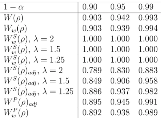
1₋α 0.90 0.95 0.99 W(ρ) 0.903 0.942 0.993 Ww(ρ) 0.903 0.939 0.994 WS w(ρ), λ= 2 1.000 1.000 1.000 WS w(ρ), λ= 1.5 1.000 1.000 1.000 WS w(ρ), λ= 1.25 1.000 1.000 1.000 WS_{(ρ)adj, λ= 2 0.789 0.830 0.883} WS_{(ρ)adj, λ= 1.5 0.849 0.906 0.958} WS_{(ρ)adj, λ= 1.25 0.886 0.937 0.982} WP_(ρ) adj 0.895 0.945 0.991 WP w(ρ) 0.892 0.938 0.989

Table 1: Equicorrelated multivariate normal model. Empirical coverage of(1₋α)

confidence intervals based on different statistics, based on 5.000 replications, with

n= 30,q = 10, ρ= 0.5, and λ= 2,1.5,1.25.

ratio statistics has reasonable coverage properties. Note that the pairwise log-likelihood, as an example of composite log-log-likelihood, is a special case of a proper scoring rule.

Table 1 reports the empirical coverages of confidence intervals based on several statistics: the full likelihood ratio W(ρ), the Wald statistic from the full model

Ww(ρ), the Tsallis Wald statistic WwS(ρ) and the adjustment (23) of the Tsallis empirical score likelihood ratio statistic WS_(ρ)

adj for three values of λ. Finally, also the pairwise Wald statistic WP

w(ρ) and the adjustment (23) of the pairwise likelihood ratio statisticWP_(ρ)

adjare given. We note that the proposed adjustment (23) ofWS_{(ρ)shows a reasonable performance in terms of coverage. In particular,} whenλ is small, it proves to be a good competitor of the pairwise likelihood ratio statistic WP_{(ρ)adj, with the advantage of using the full likelihood. However the} Tsallis Wald statistic WS

w(ρ)appears useless.

Example 6.2 Scale and location model

Let θ = (µ, σ), where µ _∈ IR is a location parameter and σ > 0 a scale parameter. In this case we have p(x;θ) = p0_{(x₋ µ)/σ_}/σ, where p0(_·) is the standard distribution. The Tsallis empirical score is S(θ) = Pn_i=1S(xi, θ), with

S(xi, θ) =−γ p(xi;θ)(γ−1)+

(γ₋1) σ(γ−1)

Z

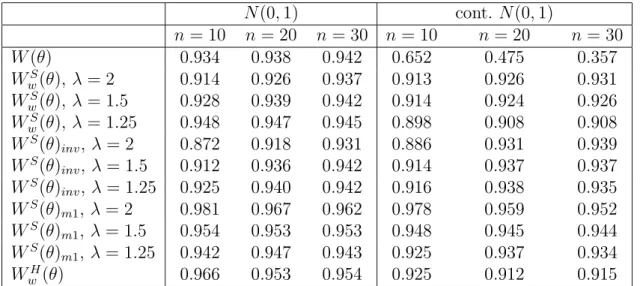
N(0,1) cont. N(0,1) n= 10 n= 20 n = 30 n= 10 n= 20 n= 30 W(θ) 0.934 0.938 0.942 0.652 0.475 0.357 WS w(θ), λ= 2 0.914 0.926 0.937 0.913 0.926 0.931 WS w(θ), λ= 1.5 0.928 0.939 0.942 0.914 0.924 0.926 WS w(θ), λ= 1.25 0.948 0.947 0.945 0.898 0.908 0.908 WS_(θ) inv, λ= 2 0.872 0.918 0.931 0.886 0.931 0.939 WS_(θ) inv, λ= 1.5 0.912 0.936 0.942 0.914 0.937 0.937 WS_(θ) inv, λ= 1.25 0.925 0.940 0.942 0.916 0.938 0.935 WS_(θ) m1,λ = 2 0.981 0.967 0.962 0.978 0.959 0.952 WS_(θ) m1,λ = 1.5 0.954 0.953 0.953 0.948 0.945 0.944 WS_(θ) m1,λ = 1.25 0.942 0.947 0.943 0.925 0.937 0.934 WH w (θ) 0.966 0.953 0.954 0.925 0.912 0.915

Table 2: Scale and location model. Empirical coverages (based on 5000 replica-tions) of 0.95 confidence regions based on different statistics, under the N(0,1)

model and the 0.95_· N(0,1) + 0.05_·N(0,102_{) contaminated model, with λ =} 2,1.5,1.25.

for i= 1, . . . , n.

We ran a simulation experiment, for several values ofnand withλ= 2,1.5,1.25, in order to assess the quality of the proposed adjustments of the Tsallis scoring rule ratio statistic based on S(θ). For comparison, we considered also the well-known Huber location-scale M-estimator (see Hampel et al., 1986, Sec. 4.2). For this estimator, only the Wald type statistic WH

w (θ) is available.

Table 2 gives the results of a Monte Carlo experiment that compares confidence regions for θ based on the full likelihood ratio W(θ), the Tsallis Wald statistic

WS

w(θ)and the adjustments (23) and (24) of the Tsallis empirical score likelihood ratio statistic, and the Huber Wald statistic WH

w (θ), when the central model is the normal one. Data are generated from two different distributions: the N(0,1)

model, and the contaminated model 0.95_·N(0,1) + 0.05_·N(0,102_{). We note}

that the proposed adjustments ofWS_{(θ)show a reasonable performance in terms} of coverage, both under the central model and under the contaminated model. However, the Tsallis Wald statistic WS

w(θ) and the Huber Wald statistic WwH(θ) exhibit poor coverage under the contaminated model.

Example 6.3 Linear regression model

Consider the linear regression model

y=Xβ+σε , (28)

whereXis a fixedn_×pmatrix,β _∈IRp _{(p≥1)an unknown regression coefficient,}

σ > 0 a scale parameter and ε an n-dimensional vector of random errors from a standard normal distribution. We take σ = 1 as known. The Tsallis empirical score is S(β) = Pn_i=1S(yi, β), with

S(yi, β) =− γ (√2π)γ−1 exp −γ−₂ 1(yi−xTiβ)2 + (γ₋1) Z φ(x)γdx , where xT

i is the i-th row of X and φ(·) is the standard normal density.

In order to assess the quality of the proposed adjustments of the Tsallis scoring rule ratio statistic based on S(β), we ran a simulation experiment with p= 3 and for several values of n, with λ = 2,1.5,1.25. For comparison, we considered also the well-known Huber regression M-estimator (see Hampel et al., 1986). As in the previous example, for this estimator only the Wald type statistic WH

w(β) is available.

Our specific model is as follows. In (28), all entries of the first column of X

are 1, those of the second column are generated as independent standard normal variables, z1, . . . , zn, while the third column consists of the integers from 1 to n. The model is yi = β1 +β2zi +β3i+εi, and the true parameter is β = (1,2,3). As for Example 6.2, ε1, . . . , εn were generated from one of two distributions: the

N(0,1) model, or the contaminated model0.95_·N(0,1) + 0.05_·N(0,102_).

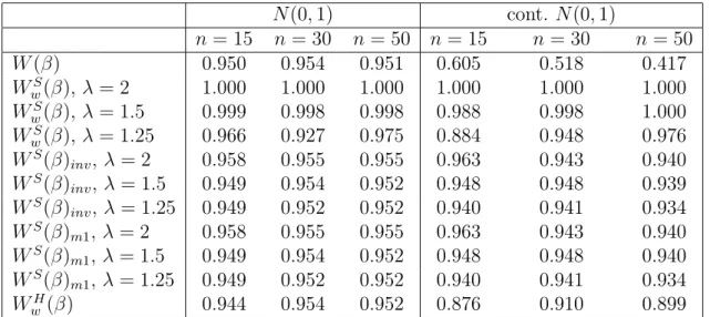
Table 3 compares confidence regions for β based on the full likelihood ratio

W(β), the Tsallis Wald statistic WS

w(β) and the adjustments (23) and (24) of the Tsallis empirical score likelihood ratio statistic, and the Huber Wald statistic

WH

w (β), when the central model is the normal one. We note that the proposed adjustments of WS_{(θ) show a satisfactory performance in terms of coverage, in} particular when λ is small, both under the central model and under the contam-inated model. However the Tsallis Wald statistic WS

w(ρ) and the Huber Wald statistic WH

N(0,1) cont. N(0,1) n= 15 n= 30 n = 50 n= 15 n= 30 n= 50 W(β) 0.950 0.954 0.951 0.605 0.518 0.417 WS w(β),λ = 2 1.000 1.000 1.000 1.000 1.000 1.000 WS w(β),λ = 1.5 0.999 0.998 0.998 0.988 0.998 1.000 WS w(β),λ = 1.25 0.966 0.927 0.975 0.884 0.948 0.976 WS_{(β)inv, λ= 2 0.958 0.955 0.955 0.963 0.943 0.940} WS_{(β)inv, λ= 1.5 0.949 0.954 0.952 0.948 0.948 0.939} WS_{(β)inv, λ= 1.25 0.949 0.952 0.952 0.940 0.941 0.934} WS_(β) m1, λ= 2 0.958 0.955 0.955 0.963 0.943 0.940 WS_(β) m1, λ= 1.5 0.949 0.954 0.952 0.948 0.948 0.940 WS_(β) m1, λ= 1.25 0.949 0.952 0.952 0.940 0.941 0.934 WH w (β) 0.944 0.954 0.952 0.876 0.910 0.899

Table 3: Linear regression model. Empirical coverages (based on 5000 replications) of 0.95 confidence regions based on different statistics, under the N(0,1) and the

0.95_·N(0,1) + 0.05_·N(0,102_{) models, with λ= 2,1.5,1.25.}

7

Concluding remarks

We have presented a general approach to parametric estimation theory, based on replacing the full log-likelihood by a proper scoring rule. This includes well-studied cases such as full, pseudo, composite, pairwise . . . log-likelihoods, as well a very wide variety of other cases, not directly or indirectly related to likelihood at all. Under smoothness conditions, any proper scoring rule can be applied to any statistical model, and delivers an associated M-estimator. While this may lose efficiency in comparison with full likelihood methods, it can exhibit improved robustness or computational advantages. In § 5 we identified some common situ-ations where use of an appropriate scoring rule achieves B-robustness.

We can use a scoring-rule estimator to construct hypothesis tests and confi-dence intervals. In addition to obtaining analogues of the Wald and score test statistics, which are available for general M-estimators, when basing inference on a scoring rule we also have an analogue of the Wilks (log-likelihood ratio) statistic. The distributions of these analogues differ from those based on the full likelihood, and we have considered adjustments to bring them more into line. The

statistics yield confidence regions whose coverage properties are satisfactory. Both the moment-matching correction and the correction given in Theorem 4.3 perform well, and are preferred to the use of Wald type statistics.

In more realistic applications, analytic expressions for the required terms K

and J may be unavailable, and numerical evaluation would then seem to offer the most straightforward solution. This issue is under investigation.

A

Boundedness

Lemma A.1 Let P be a distribution onR, with differentiable probability density

function f(_·). Suppose _|f′_{(x)| ≤K, all x. Then f(x)≤1 + 2K.}

Proof. Define

A− := _{x:f(x)_≤1_}

An := {x: 2n < f(x)≤2n+1} (n = 0,1, . . .).

Then Ris the disjoint union of these sets.

We have1_≥P(An)≥2nλ(An), whereλis Lebesgue measure. Soλ(An)≤2−n. On An, the total variation off does not exceed K_×λ(An)≤K×2−n. Hence the total variation outside A− is at most K×P∞0 2−n = 2K. ✷

References

[1] Barndorff-Nielsen, O. E. & Cox, D. R. (1994), Inference and Asymptotics. Chapman & Hall, London.

[2] Basu, A., Harris, I. R., Hjort, N. L. & Jones, M. C. (1998). Robust and efficient estimation by minimising a density power divergence. Biometrika 85, 549–559.

[3] Bernardo, J. M. (1979). Expected information as expected utility. Ann. Statist. 7, 686–690.

[4] Besag, J. E. (1975). Statistical analysis of non-lattice data. J. Roy. Statist. Soc. D 24, 179–195

[5] Brier, G. W. (1950). Verification of forecasts expressed in terms of probabil-ity. Monthly Weather Rev.78, 1–3.

[7] Cox, D. R. & Reid, N. (2004). A note on pseudolikelihood constructed from marginal densities. Biometrika 91, 729–737.

[8] Dawid, A. P. (1986). Probability forecasting. In Encyclopedia of Statistical Sciences (S. Kotz, N. L. Johnson, C. B. Read, eds.), 7. Wiley-Interscience, 210–218

[9] Dawid, A. P. (2007). The geometry of proper scoring rules. Ann. Instit. Statist. Math. 59, 77–93.

[10] Dawid, A. P. & Lauritzen, S. L. (2005). The geometry of decision theory. In

Proceedings of the Second International Symposium on Information Geome-try and its Applications. University of Tokyo, 22–28.

[11] Dawid, A. P. & Musio, M (2013). Estimation of spatial processes using local scoring rules. Adv. Statist. Anal. 97, 173-179.

[12] Dawid, A. P. & Musio, M (2014). Theory and applications of proper scoring rules. Metron, to appear.

[13] Gneiting, T. & Raftery, A. E. (2007). Strictly proper scoring rules, prediction, and estimation. J. Amer. Statist. Assoc.102, 359–378.

[14] Godambe, V. P. (1960). An optimum property of regular maximum likelihood equation.Ann. Statist. 31, 1208–1211.

[15] Good, I. J. (1952). Rational decisions. J. Roy. Statist. Soc.B 14, 107–114 . [16] Hampel, F. R., Ronchetti, E. M., Rousseeuw, P. J. & Stahel, W. A. (1986).

Robust Statistics: The Approach Based on Infuence Functions. John Wiley and Sons, New York.

[17] Heritier, S. & Ronchetti, E. (1994). Robust bounded-influence tests in general parametric models. J. Amer. Statist. Assoc. 89, 897–904.

[18] Huber, P. J. & Ronchetti, E. M. (2009). Robust Statistics. John Wiley and Sons, New York.

[19] Hyvärinen, A. (2005). Estimation of non-normalized statistical models by score matching.J. Machine Learning 6, 695–709.

[20] Kent, J. T. (1982). Robust properties of likelihood ratio tests. Biometrika 69, 19–27.

[21] Lindsay, B., Pilla, R. & Basak, P. (2000). Moment-based approximations of distributions using mixtures: Theory and applications. Ann. Inst. Statist. Math. 52, 215–230.

[22] McCarthy, J. (1956). Measures of the value of information.Proc. Nat. Acad. Sci. USA 42, 654–655.

[23] Molenberghs, G. & Verbeke, G. (2005). Models for Discrete Longitudinal Data. Springer, New York.

[24] Pace, L., Salvan, A. & Sartori, N. (2011). Adjusting composite likelihood ratio statistics. Statist. Sinica 21, 129–148.

[25] Pace, L., Salvan, A. & Sartori, N. (2013). Adjusted pseudo composite likeli-hood ratios.Proc. 28th IWSM, Palermo, 723–726.

[26] Parry, M. F., Dawid, A. P. & Lauritzen, S. L. (2012). Proper local scoring rules. Ann. Statist. 40, 561–592.

[27] Rotnitzky, A. & Jewell, N. (1990). Hypothesis testing of regression parame-ters in semiparametric generalized linear models for cluster correlated data.

Biometrika77, 485–497.

[28] Satterthwaite, F. E. (1946). Approximate distribution of estimates of vari-ance components. Biometrics Bull. 69, 110–114.

[29] Savage, L. J. (1971). Elicitation of personal probabilities and expectations.

J. Amer. Statist. Assoc.66, 783–801.

[30] Varin, C. (2008). On composite marginal likelihood. Adv. Statist. Anal. 92, 1–28.

[31] Varin, C., Reid, N. & Firth, D. (2011). An overview of composite likelihood methods. Statist. Sinica 21, 5–42.

[32] Wood, A. (1989). An F approximation to the distribution of a linear com-bination of chi-squared variables.Comm. Statist. Simul. Comput. 18, 1439– 1456.