CS-SFD Algorithm for GNSS Anti-Jamming Receivers
Fulai Liu1, 2, *, Lei Liu1, 2, Jiaqi Yang1, 2, and Miao Zhang1, 2
Abstract—Most of space-time adaptive processing methods have the excellent ability to suppress interferences when the space-time covariance matrix is perfectly estimated. Unfortunately, these methods may have calculation error of the covariance matrix in the case of fewer snapshots, which may lead to remarkable performance degrading. To solve the aforementioned problem, a space-frequency domain anti-jamming algorithm based on the compressed sensing theory (CS-SFD) is presented. Firstly, the proposed method utilizes less sampled data to form a space-frequency two-dimensional sparse representation for the narrowband interference signals. Secondly, the interference covariance matrix estimation problem is modeled as a sparse reconstruction problem which can be efficiently solved by the orthogonal matching pursuit algorithm. Furthermore, the diagonal loading method is used to modify the interference plus noise covariance matrix. Finally, the weight vector is given by the minimum output power criterion. Compared with the previous work, the presented method has better robustness and more effectively anti-jamming performance in the case of fewer snapshots. Simulation results show the effectiveness of the proposed algorithm.
1. INTRODUCTION
Global navigation satellite system (GNSS) plays a very important role in providing global users with 24/7 service such as positioning, timing and navigation. With increasingly fierce military confrontation, the potential security threat to satellite navigation becomes an intractable problem [1]. Taking global positioning system (GPS) as an example, the frequency and modulation mode of existing GPS signals are available for public, and due to the weak power level when GPS signals arrive at the ground [2], it is effortless to be interfered or deceived for GPS signals. Space-time adaptive processing (STAP), which was first proposed by Forst in 1972, can suppress interferences by controlling the gain and phase of each array element in the array to produce nulls in the direction of interference [3]. Classic array weighting criteria include minimum variance distortionless response (MVDR) criteria, power inversion (PI) criteria, etc., which are the basis of STAP [4, 5]. In 2000, Fante and Vacarro comprehensively discussed the application of STAP processing technology in GNSS receiver anti-interference [6], making STAP the main technique of GNSS anti-interference.
As one of the most effective GNSS anti-jamming technologies, STAP extends one-dimensional time-domain, frequency-domain, and spatial filtering to form a space-time two-dimensional processing structure, which greatly increases the degree of freedom (DOF) of the array without increasing the number of array elements, thereby increasing the number of interferences that can be processed [7]. Therefore, STAP-based GNSS anti-jamming technology has been extensively studied, and a series of results are achieved. Part of the studies, optimizing the space-time array structure to increase DOF, introduce polarization arrays [8] and sparse array structures [9] into STAP. In addition, to make STAP technology easier to implement in hardware, an algorithm focused on low-complexity STAP algorithms
Received 10 December 2018, Accepted 15 February 2019, Scheduled 1 March 2019 * Corresponding author: Fulai Liu ([email protected]).
based on multi-level Wiener filtering is proposed in [10]. Unfortunately, there are inevitable errors and disturbances in practical applications such as high dynamic environments and multipath environments, which may lead to deterioration of STAP performance. To solve this problem, a series of STAP robust optimization algorithms have been proposed. Based on the space-time method of multi-beamforming, [11] proposes a robust STAP algorithm based on quadratic cone programming, which can suppress multipath interferences and other interferences. To further improve the robustness of the beamformer, a nonuniform diagonal loading method is used in [12], which improves the noise suppression capability of beamforming through changing the diagonal load adaptively referring to the input signal-to-noise ratio (SNR). For various robust anti-interference algorithms, whether the covariance matrix is solved accurately has a great influence on the performance of the algorithm. Several STAP algorithms based on covariance matrix reconstruction are proposed to improve beamforming performance to solve this problem [13–15]. In addition, an algorithm for the null broadening with respect to the nonstationary interference is proposed [16], which can reconstruct clutter plus noise covariance matrix (CNCM) accurately and have significant anti-interference performance.
The computational cost and memory usage brought about by the inverse matrix of CNCM, which grow rapidly with an increase of problem’s dimension, cannot be ignored. The above calculation methods have not considered using the sparse characteristics of the signal itself to overcome the adverse effects of fewer snapshots either. In 2007, compressive sensing (CS) was applied by Baraniuk in the field of communications, which can capture and represent compressible signals at a rate significantly below the Nyquist rate [17]. There are quite a few excellent CS algorithms that have been proposed such as the orthogonal matching pursuit (OMP) algorithm [18] and Bayesian compressive sensing [19]. Most recently, sparse representation based STAP (SR-STAP) methods have been extensively researched in the field of radar [20–22]. Inspired by the above successful applications, a GNSS space-frequency domain anti-jamming algorithm based on the compressed sensing theory (CS-SFD) is proposed. The algorithm uses less sampled space-time two-dimensional data to solve the spacefrequency two-dimensional spectral function of the interference signal through the compressed sensing reconstruction algorithm and estimates the covariance matrix according to the null spectrum function, so as to obtain the anti-interference weight vector, which has better robustness under fewer snapshots. The rest of the paper is organized as follows. The data model is described in Section 2. Section 3 introduces the proposed method. Section 4 gives some simulation results. Finally, the conclusion is summarized in Section 5.
2. SYSTEM MODEL
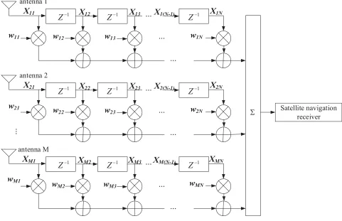
Assuming that GNSS signals and interference signals are both far-field signals. A standard implementation of the STAP model is shown in Figure 1. Consider that there is a uniform linear array (ULA) with M antennas and tapped delay lines (TDLs) with N taps in this model. The delay time of TDL is usually employed as a sampling duration and denoted by Ts, and the first element of the ULA is employed as the phase reference. Without loss of generality, assume that the reception, composed of one GNSS signal and J narrowband compression interferences, can be expressed as
x(t) =αs(θs, fs)aS+
j=J
j=1
βj(θj, fj)aj+n(t) (1)
where x(t) = [x11(t), x12(t), . . . , x21(t), x22(t), . . . , xM N(t)]T is the received signal vector at time t, and [·]T denotes the transpose of [·]. αs(θs, fs) and βj(θj, fj) represent the amplitude of the GNSS signal and the j-th interference signal. n(t) denotes the white Gaussian noise. aS = aS(θ, f) represents the spatial-temporal steering vector of the GNSS signal, and aj(t) =aJ(θj, fj) is thej-th spatial-temporal steering vector of interference signal. A space-time steering vector aJ(θ, f) can be given as
a(θ, f) =a(θ)⊗a(f) (2) where a(θ) = [1, e−j2πdλ, . . . , e−j2π(M−1)
d
λ]T, a(f) = [1, e−j2πf T, . . . , e−j2π(N−1)f T]T, a(θ) and a(f) are
X11 X12 X13 ...X1(N-1) X1N
...
...
w11 w12 w13 w1N
1
Z
− 1Z
− 1Z
−antenna 1
X21 X22 X23 ...X2(N-1) X2N
...
...
w21 w22 w23 w2N
1
Z
− 1Z
− 1Z
−antenna 2
XM1 XM2 XM3 ...XM(N-1) XMN
...
...
wM1 wM2 wM3 wMN
1
Z
− 1Z
− 1Z
−antenna M
Σ
...
Satellite navigation receiver
Figure 1. Space-time joint anti-interference model.
Hence, the data samples collected at timetat the receiver can be expressed as
xJ =
J
j=1
βj(θj, fj)a(θj, fj) (3)
where βj(θj, fj) denotes the complex amplitude of the j-th narrowband suppressive interfering signal. Rj =E[xJxHJ] is the real interference covariance matrix, where (·)H denotes the conjugate transpose, andE[·] denotes the expectation. Rj+n=Rj+σ2I is the real interference-plus-noise covariance matrix
whereI is the unit diagonal array. Then choose the appropriate calculation criteria to get the optimal weight vector of the array. Hence, the output of the space-time adaptive processor can be obtained as
y=wHx (4)
where wH = [w11, w12, . . . , w1N, w21, . . . , w2N, . . . , wM N], wM N denotes the weight at the n-th tap of
them-th antenna element, and (·)H denotes the conjugate transpose.
3. ALGORITHM FORMULATION 3.1. Interference Signal Sparsity
are divided intoNd bands. Therefore, g is anNf ×Nd dimensional matrix, which is shown as follows g= ⎡ ⎢ ⎢ ⎢ ⎢ ⎢ ⎣
0 0 0 . . . 0 0 αs 0 . . . β0
0 ... . . . β1 β2 ..
. β2 0 . . . ... β3 0 0 . . . 0
⎤ ⎥ ⎥ ⎥ ⎥ ⎥ ⎦ (5)
where α and β represent the complex amplitudes of each satellite signal and interference signal, and the position subscript in the matrix corresponds to the frequency band and the direction of arrival after discretization in the space frequency domain.
Consider that the interference signals received by the receiver are narrow-band compression interferences and that the number of interference sources is limited. Since the satellite signals arrive at the receiver weak and submerged in noise, the space-frequency spectrum of the received signals has the following form g= ⎡ ⎢ ⎢ ⎢ ⎢ ⎢ ⎣
σn σn σn . . . σn σn σn σn . . . β0
σn ... . . . β1 β2 ..
. β2 σn . . . ...
β3 σn σn . . . σn ⎤ ⎥ ⎥ ⎥ ⎥ ⎥ ⎦ (6)
whereσn represents the amplitude of the space-frequency spectrum of Gaussian white noise. It is easy to find in Eq. (6) that only a few β elements have significant values and are related to the interference signal, while the remaining β elements have small values and are related to noise. When the noise power in the interference power domain is larger than that in the value, it is easy to find that the space-frequency spectrum of the received signal is sparse.
3.2. Covariance Matrix Recovery
Different from the traditional STAP method, the sparse spectral recovery structure STAP method (SR-STAP) in the case of uniform linear array is first proposed in the literature [23] in 2009. This method is used for clutter suppression of radar echo signal. The space-frequency spectrum of detection unit clutter is estimated firstly, and then the covariance matrix is estimated by the space-frequency spectrum. The SR-STAP method can obtain good performance of wavelet suppression. Compression interference suppression in navigation satellite system has something in common with radar clutter suppression.
According to the space-time array model, the data received byN tapped space-time array antennas in a single snapshot ofM array elements isxin Eq. (3), andxis theM N×1 dimensional vector. The angles and frequencies are discretized at intervals. Select an angle interval of Δθ and an initial value of θ0, and select a total ofNd points. Set the initial frequency value asf0 and the discrete interval as Δf, and select a total of Nf points. The space-frequency spectrum is rewritten as NdNf ×1 dimensional column vector g, and the data received by the space-time adaptive array has the following relationship with the space-frequency spectrum of the received signal.
x=Φg+n (7)
where n is the noise vector. Φ, formed by space-time steering vectors, is the basic matrix whose dimension isM N×NdNf. Each column ofΦcorresponds to a steering vector, and each steering vector atom corresponds to a different (θ, f) value. Because of the discretization of the space domain and frequency domain, it is obvious thatM N NdNf is needed to ensure that the basic matrix atoms are complete enough. Eq. (7) is a typical sparse recovery model of compression perception, so the problem of space-frequency spectrum estimation can be transformed into the sparse recovery problem as follows
min||g||1
s.t.||x−Φg||2 ε (8)
theory, Eq. (8) can be solved by using OMP algorithm. OMP algorithm, also known as orthogonal matching pursuit algorithm [24], is one of the more classic greedy algorithms. The core idea of the OMP algorithm is to gradually determine the position of non-zero elements of the sparse coefficient vector by calculating the correlation degree between each column of the dictionary matrix Φand the sparse coefficient vectorg. Assuming that the support set of vectorg is Γ = supp(g) ={i:gi = 0}, the most relevant column of vector in Φis selected as the atom in each iteration to be incorporated into the candidate support set. If the signal sparsity is K, at least K iterations are needed to accurately restore the source signal. Therefore, within a certain range, as the number of iterations increases, the reconstructed signal will be closer and closer to the source signal. In practical application, it is usually determined that the number of iterations is the sparse degree K, or a certain reconstruction error is given. When the number of iterations reaches K, or the reconstruction error meets the conditions, the loop terminates.
After obtaining the estimation of the support set, the estimated value of the sparse coefficient vector can be obtained by solving Equation (9)
ˆ
g=Φ†Γx (9)
where Φ†Γ = (ΦTΓΦΓ)−1ΦTΓ, which is called the pseudoinverse of ΦΓ. Therefore, the OMP algorithm can be regarded as a least square estimation problem. The steps of the OMP algorithm are described as follows.
Table 1. OMP algorithm steps.
(1) Input perception matrixΦ, observation signalx and error toleranceε;
(2) Initialize residualr0=x, support setΓ0 =∅,Φ0=∅, and iteration numberl= 1;
(3) calculate λl,λl = argmax|rl−1, φ|(i= 1,2, . . . , N), where λrepresents the elements of the support set;
(4) Let Λl=Λl−1∪λl,Φl=Φl−1∪φl;
(5) Find the least squares solution ofx=Φlgl: ˆg=argmin
gl
||x−Φlgl||= (ΦlTΦl)−1ΦTlx;
(6) Update the residualrl=x−Φlˆgl=x−Φl(ΦTl Φl)−1ΦTl x;
(7) Let l=l+ 1, if||rl|| ≥ε, jump to step (3), otherwise the cycle ends;
(8) The restored support set isΛl, and the recovered signal is ˆgl obtained by the last iteration; (9) After the sparse coefficient vector ˆg is restored.
∅indicates an empty set, andrl−1, φdenotes the inner product operation of the two elements in Table 1. After the space-frequency spectrum of the interference signals solved by the OMP algorithm, another important step is to establish the connection between the space-frequency spectrum and the covariance matrix of interference signals. According to Eq. (7), the CCM obtained based on the recovered space-frequency spectrum can be expressed as follows
Rx = ExxH= EΦggHΦH=ΦEggHΦH =
NdNf
i=1
|gi|2φiφHi + NdNf
i=1
NdNf
i=1,j=1
gig∗jφiφHj (10)
covariance matrix modified by the diagonal loading technique to correct the sampling covariance matrix can be expressed as
Rx=Rx+λDLI (11)
where λDL is the loading value, and I is the unit diagonal matrix. With diagonal loading, select the appropriate loading value λDL. Then the large eigenvalues corresponding to strong interference will not be significantly affected, while the small eigenvalues corresponding to noise will be increased and compressed near λDL [15]. Therefore, the CS-SFD algorithm presented in this paper can obtain better noise suppression effect. The loading quantity selected in this chapter is the estimated value of noise power, which can be estimated by the noise level in the non-interference environment in practical application, and the noise power can be obtained for diagonal loading.
3.3. Anti-Jamming Beamforming
After calculating the estimated value of the covariance matrix, beamforming is required. The filter weight coefficient obtained by beamforming is used for interference suppression. Since the GNSS signal power is lower than the noise power, it is not necessary to consider adjusting the main beam to align it with the direction of arrival of the desired signal. The minimum output power criterion is selected for beam formation, and the constraint setting ensures that the GNSS signals in the field of view are as non-distorted as possible, and the interference is largely suppressed. The optimization problem can
be described as follows
min
w w HR
xw
s.t.wHh= 1 (12)
According to the Lagrangian multiplier method and the estimated covariance matrix, the optimal solution of the weight vector can be obtained as
wopt = R −1
x h
hHR−x1h (13)
where h = [1,0,0, . . . ,0]T. Through the above analysis, the steps of the cs-stf algorithm can be summarized as Table 2.
Table 2. CS-SFD algorithm steps.
Stap 1: Obtain the single shot data of the space-time array and conduct vectorization on it to get sampled signal;
Stap 2: Discretize the direction domain and frequency domain at proper interval according to the space-time anti-interference target; construct the matrix of overcomplete space-fre--quency steering vector Φ;
Stap 3: Solve the estimated valueg of the interference space-frequency spectrum by the OMP algorithm and obtain the information of the interference signals (θ, f);
Stap 4: Use the estimated value of the interference space spectrum calculate the interference covariance matrixRx, and select the loading quantity to deal withRx to improve the robustness to noise;
Stap 5: Calculate the optimal weight wopt by using Equation (13) to form the beam.
4. SIMULATION AND ANALYSIS
parameters. The performance difference between the proposed algorithm and the classical MVDR al-gorithm and PI alal-gorithm is compared, and the simulation results are analyzed. Consider a ULA with M = 4 array elements, and each element is equally spaced with N = 7 taps. The distance between the array elements of the ULA is half the wavelength of the GNSS signal. Consider that the received signal contains a GNSS signal as the desired signal and three narrowband suppressed interference sig-nals. The carrier modulation mode of the GNSS signal is BPSK. In order to simplify the simulation, it is assumed that the GNSS receiver performs signal processing with a center frequency of 40 MHz and a signal bandwidth of 20 MHz. The number of interferences is 3, and all of them are narrow-band suppressed interferences, whose (f, θ) values are (1.2,0),(0.8,−50),(1,30), respectively, and the interference-to-signal-ratios (ISRs) are 45 dB, 45 dB and 40 dB, respectively. According to the Nyquist sampling theorem, the sampling frequency is set to 4 times the center frequency of the signal.
(1) Comparison of array orientation diagram
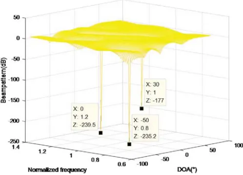
Figures 2–4 show the array patterns of CS-SFD algorithm, PI algorithm, and MVDR algorithm, respectively. The number of snapshots of MVDR algorithm and PI algorithm in the experiment is K = 4. It can be seen that the CS-SFD algorithm forms deeper nulls at the corresponding interference
Figure 2. Beam pattern of CS-SFD.
directions and frequencies, and the depths of the depressions are −200 to −100 dB, while the beam pattern in the other directions is smoother. The above situations occur because the reconstructed in-terference null spectrum contains only the direction of arrival (DOA) and frequency information of the interferences, so that the deep nulls can be accurately formed, and the generation of the pseudo null and the distortion of the beam pattern are avoided. Although MVDR algorithm and PI algorithm form nulls in the interference directions and frequencies, the depths of the nulls are about −40 to −30 dB, which are significantly smaller than the CS-SFD algorithm. And the number of snapshots used in the calculation is small, which makes the covariance matrix estimation of MVDR algorithm and PI algo-rithm not accurate, resulting in a certain degree of pattern distortion.
(2) The anti-interference performance of the CS-SFD algorithm when the input ISR changes
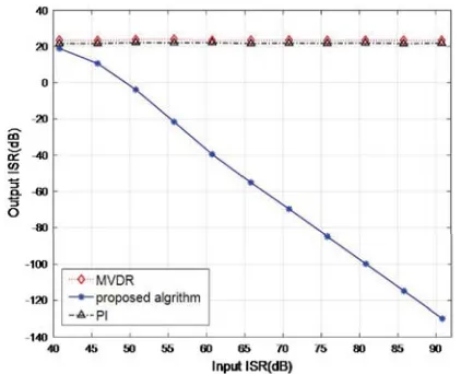
Figures 5 and 6 show the output ISR and signal-to-interference-plus-noise-ratio (SINR) curves of each algorithm. The input ISR is changed from 40 dB to 90 dB in Figure 5 and 20 dB to 70 dB in Figure 6. Each point on the curves is obtained by 1000 Monte Carlo experiments. According to Figure 5, as the input ISR increases, the output ISRs of MVDR algorithm and PI algorithm are both stable at around 20 dB, while the CS-SFD algorithm uses the reconstructed space-frequency spectrum to estimate the CCM with the interference power. Under these circumstances, the amplitude of the interfering signals in the reconstructed space-frequency spectrum will be larger with the increase of input ISR. When adaptive beamforming is performed, a deeper null will be generated, and a better interference suppression effect is obtained. According to Figure 6, under the current simulation conditions, the CS-SFD algorithm has the highest output SINR, which is significantly higher than MVDR algorithm and PI algorithm. This is because MVDR algorithm and PI algorithm use the snapshot data to solve the problem when the number of snapshots is small. The variance matrix does not accurately contain interference and noise information. The CS-SFD algorithm is more thorough in suppressing interference, thus the output SINR is higher than the other two algorithms.
Figure 5. Output INR versus input ISR. Figure 6. Output SINR versus input ISR.
(3) Comparison of the anti-interference performance between the single-shot CS-SFD algorithm and multi-shot MVDR/PI algorithm
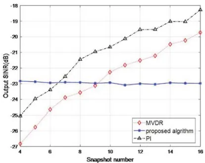
The output ISR and output SINR of CS-SFD, MVDR, and PI are simulated experimentally, where the input ISR is 60 dB. Among them, the snapshot numbers of MVDR algorithm and PI algorithm change from 4 to 16, while the CS-SFD algorithm is in the case of single snapshot. The other basic simulation conditions are the same as the previous experiments.
Figure 7. The output INR versus snapshot number.
Figure 8. The output SINR versus snapshot number.
whose simulation condition is the change of the number of snapshot and the CS-SFD algorithm whose simulation condition is the single snapshot. According to Figure 7, with the increase of number of snapshots, the covariance matrices of MVDR algorithm and PI algorithm are more and more accurate, and the output ISR shows a downward trend, but the anti-interference performance is still slightly inferior to that of the CS-SFD algorithm. According to Figure 8, when the number of snapshots is small, the output SINR of the CS-SFD algorithm is superior to the other two algorithms. With the increase of snapshot number, the covariance matrix of MVDR algorithm and PI algorithm can better reflect the noise information, so the two algorithms are better than the CS-SFD algorithm proposed.
5. CONCLUSION
In this paper, in order to solve the problem that fewer snapshots are easy to cause inaccurate covariance matrix estimation and that the performance of the anti-jamming algorithm is degraded, a space-time anti-interference algorithm based on the compressed sensing theory under fewer snapshots is proposed. The algorithm only needs a few space-time snapshots data to recover the space-frequency spectrum of the interference signal through the compressed sensing reconstruction algorithm, and then construct the interference signal covariance matrix to calculate the weight. By using the diagonal loading technique, the noise suppression capability of the algorithm can be improved, and the narrowband suppressed interference in the received signal can be effectively suppressed. The simulation results show that compared with the traditional space-time adaptive anti-jamming algorithm, the proposed algorithm can achieve better anti-interference effect and has certain robustness by using less data.
ACKNOWLEDGMENT
This work was supported by the Natural Science Foundation of Hebei Province (Grant No. F2016501139) and the Fundamental Research Funds for the Central Universities (Grant No. N172302002 and No. N162304002).
REFERENCES
1. Kaplan, D. E. and C. Hegarty, Understanding GPS: Principles and Application, Artech House Publishers, Massachusetts, USA, 2005.
3. Frost, III, L. O., “An algorithm for linearly constrained adaptive array processing,”Proceedings of the IEEE, Vol. 60, No. 8, 926–935, 1972.
4. Widrow, B., P. E. Mantiey, L. J. Griffiths, and B. B. Goode, “Adaptive antenna systems,”
Proceedings of the IEEE, Vol. 55, No. 12, 2143–2159, 1967.
5. Compton, R. T., “The power-inversion adaptive array: Concept and performance,” Aerospace &
Electronic Systems IEEE Transactions on AES, Vol. 15, No. 6, 803–814, 1979.
6. Fante, R. L. and J. J. Vacarro, “Cancellation of jammers and jammer multipath in a GPS receiver,”
IEEE Aerospace and Electronic Systems Magazine, Vol. 13, No. 11, 25–28, 1988.
7. Liu, F., R. Du, and X. Bai, “Virtual space-time adaptive beamforming method for space-time antijamming,”Progress In Electromagnetics Research M, Vol. 58, 183–191, 2017.
8. Fante, R. L. and J. J. Vacarro, “Valuation of adaptive space-time-polarization cancellation of interference,” 2002 IEEE Position Location and Navigation Symposium, 1–3, California, April, 2002.
9. Amin, M. G., X. Wang, Y. D. Zhang, F. Ahmad, and E. Aboutanios, “Sparse arrays and sampling for interference mitigation and DOA estimation in GNSS,”Proceedings of the IEEE, 1–16, 2016. 10. Myrick, W. L., J. S. Goldstein, and M. D. Zoltowski, “Low complexity anti-jam space-time
processing for GPS,”IEEE International Conference on Acoustics IEEE, 2001.
11. Fernandez-Prades, C. and J. A. Fernandez-Rubio, “Robust space-time beamforming in GNSS by means of second-order cone programming,”IEEE International Conference on Acoustics, 2004. 12. Li, W., B. Yang, and Y. Zhao, “Low-complexity non-uniform diagonal loading for robust adaptive
beamforming,” IEEE Applied Computational Electromagnetics Society Symposium, 2017.
13. Mu, P., D. Li, Q. Yin, and W. Guo, “Robust MVDR beamforming based on covariance matrix reconstruction,”Science China Information Sciences, Vol. 56, No. 4, 1–12, 2013.
14. Hou, Y., L. Xue, and Y. Jin, “Robust adaptive beamforming method based on interference-plus-noise covariance matrix,” IEEE International Conference on Signal Processing, 2013.
15. Liu, F., J. Wu, R. Du, and X. Bai, “Robust adaptive beamforming against the array pointing error,” 2017 Progress In Electromagnetics Research Symposium — Fall (PIERS — FALL), 2782– 2789, Singapore, November 19–22, 2017.
16. Qian, J., Z. He, J. Xie, and Y. Zhang, “Null broadening adaptive beamforming based on covariance matrix reconstruction and similarity constraint,” Eurasip Journal on Advances in Signal, Vol. 1, 1–10, 2017.
17. Baraniuk, R. G., “Compressive sensing,”IEEE Signal Processing Magazing, Vol. 24, No. 4, 118–124, 2007.
18. Tropp, J. and A. C. Gilbert, “Signal recorvery form random measurements via orthogonal matching pursuit,”IEEE Trans. iNFORM, Vol. 53, No. 6, 4655–4666, 2007.
19. Ji, S., Y. Xue, and L. Carin, “Bayesian compressive sensing,”IEEE Trans. Signal Process., Vol. 56, No. 6, 2346–2356, 2008.
20. Wu, Q., Y. D. Zhang, M. G. Amin, and B. Himed, “Space-time adaptive processing and motion parameter estimation in multistatic passive radar using sparse bayesian Learning,” IEEE Transactions on Geoscience Remote Sensing, Vol. 54, No. 2, 944–957, 2016.
21. Duan, K., Z. Wang, W. Xie, H. Chen, and Y. Wang, “Sparsity-based STAP algorithm with multiple measurement vectors via sparse bayesian learning strategy for airborne radar,”IET Signal Processing, Vol. 11, No. 5, 544–553, 2017.
22. Bai, G. T., R. Tao, J. Zhao, and X. Bai, “Parameter-searched OMP method for eliminating basis mismatch in space-time spectrum estimation,” Signal Processing, Vol. 138, 11–15, 2017.
23. Sun, K., H. Zhang, G. Li, H. Meng, and X. Wang, “A novel STAP algorithm using sparse recovery technique,”IEEE International Geoscience & Remote Sensing Symposium, 2009.