USING AN ANT COLONY OPTIMIZATION ALGORITHM FOR IMAGE EDGE DETECTION AS A THRESHOLD SEGMENTATION FOR OCR SYSTEM

(1)

ISSN: 1992-8645 www.jatit.org E-ISSN: 1817-3195

5825

AUTOMATIC CHRONOLOGICAL ORDERING OF AUDIO

DATA USING SPECTOGRAMS

1_{ALEXANDER ALFIMTSEV,} 2_{SVETLANA NAZAROVA,}3_{Xiao Zelong}

1_{Assoc. Prof., Bauman Moscow State Technical University, 105005 Moscow, Russia} 2_{PhD Student, Bauman Moscow State Technical University, 105005 Moscow, Russia}

3_{PhD, School of Electronical and Optical Engineering, Nanjing University of Science and Technology,}

Nanjing, Jiangsu Province, China.

E-mail: 1_{[email protected]}_,2_{[email protected]}

ABSTRACT

An automatic quantitative method for speech fragment analysis and chronological ordering is proposed. The method works by first converting the audio data into two-dimensional spectrograms and then extracting a large set of 1030 numerical descriptors (features) from the raw spectrograms, as well as from transforming the spectrograms. The audio fragments’ similarity value is computed using a variation of the Weighted K-Nearest Neighbour scheme. The similarity tree is then used to visualize the differences between the speech fragments. The accuracy of the method depends on the size of the feature set for the analysis and the length of the audio files. The speech fragments of the well-known politicians Vladimir Putin, Barak Obama, Angela Merkel, Jacques Chirac, George Bush and Vladimir Zhirinovsky were used for the analysis. The experimental results show that the method was able to create a chronological ordering of the speech fragments and that the most significant features for the analysis of audio data are: histograms of fuzzy-oriented gradients, multiscale histograms, and combinations of geometric moments.

Keywords: Audio analysis, Chronological ordering, Fuzzy feature, Speech fragment, Two-dimensional spectrogram

1. INTRODUCTION

The application of pattern recognition and machine learning to automatic analysis of audio data allows for the solving of many tasks. One of the most common tasks in the field of automatic analysis of audio fragments is their classification.

Classification of audio data can be done by genre [1, 2], emotional colouring of compositions [3] or dominant musical components [4]. Other directions of research in the field of automatic audio analysis include automatic music recommendations [5], cover version detection [6], sound quality prediction [7], understanding environmental cognition [8] and pure-tone audiometry [9]. An important task is also to search in audio databases for the most similar sound pieces based on an input audio sample [10– 12].

In the field of automatic analysis of speech fragments, similar tasks can be solved, such as data classification by speaker’s sex or age (for different statistical research studies), by the emotional colouring of speech, and by the record time. However, the arranging of speech fragments in

chronological order seems to be the most sophisticated task. Even a human (expert) is not always able to do it accurately enough. Automatic analysis of audio records allows for the monitoring of changes in human speech characteristics over a long period of time. These characteristics include pause characteristics, speech rate, vocal strength, voice height and tone.

(2)

5826

2. MATERIAL AND METHODS

2.1. Preparation of the input dataset

To carry out the accurate analysis and validation of the method’s work, it is necessary to have enough audio data of the recorded speech of one person, recorded over several years, of good quality. In addition, the important criterion was public access to

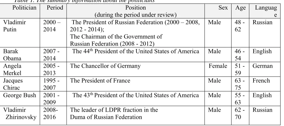
[image:2.612.96.548.226.428.2]

records. According to these assumptions the input dataset was composed of speech fragments belonging to famous politicians whose political career was at least 6 years. In this study about 460 audio records belonging to Vladimir Putin, Barack Obama, Angela Merkel, Jacques Chirac, George Bush and Vladimir Zhirinovsky were used. Table 1 represents the summary information about the politicians, whose records were used in the experiment.

Table 1. The summary information about the politicians

Politician Period Position

(during the period under review)

Sex Age Languag e Vladimir

Putin 2000 – 2014 2012 - 2014); The President of Russian Federation (2000 – 2008, The Chairman of the Government of

Russian Federation (2008 - 2012)

Male 48 -

62 Russian

Barak

Obama 2007 - 2014 The 44

th_{President of the United States of America} _Male _{46 -}

54 English Angela

Merkel 2005 - 2013 The Chancellor of Germany Female 51 - 59 German

Jacques

Chirac 1995 - 2007 The President of France Male 63 - 75 French

George Bush 2001 -

2009 The 43

th _{President of the United States of America} _Male _{55 -}

63 English Vladimir

Zhirinovsky

2008- 2016

The leader of LDPR fraction in the Duma of Russian Federation

Male 62 - 70

Russian

For each person, the input dataset was split into several periods (lasting for two or four years) starting from the person’s assumption of office of a state leader. Computer analysis in this research was based on the hypothesis that a two-year time interval is long enough to analyse it because, during this interval, a person produces a certain style of speech and performance. Also such interval is long enough to represent age voice changes. The goal of the study is to prove the possibility of automatic monitoring of these changes and the recognition of their dynamics, as well as the chronological ordering of the intervals from the input data set.

Each period includes a certain number of audio fragments recorded during the time interval under review (this number varies from 13 to 18 for different politicians). In each period, as many audio fragments where the politician answers journalists’ questions (not reading from a prepared speech) as possible were included. The reason is that such type of data reflects the characteristics of the person’s speech in a certain time interval more accurately.

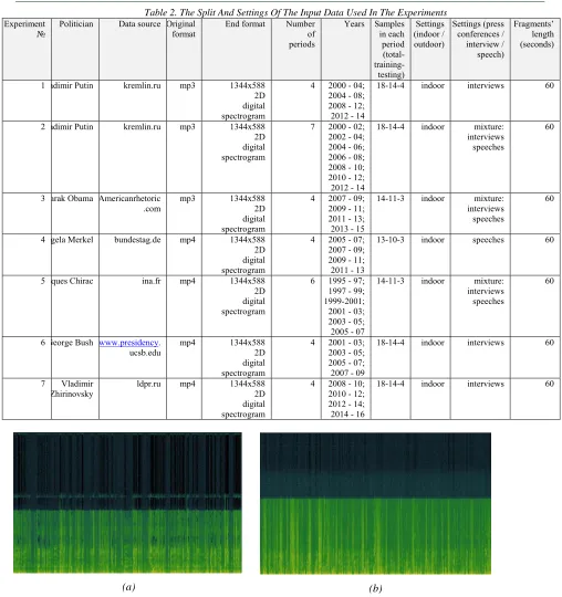
Audio fragments were originally FLAC (eng. Free Lossless Audio Codec) and then were converted to WAV (eng. Waveform Audio File Format). To normalize audio fragments by their length, each audio file was cut to 60 seconds using a free online converter «online-convert.com». These fragments do not include the entire speech, but they are long enough to analyse the speech characteristics. Audio files were chosen such that they had no background noise (outside talks, applause, equipment noise, etc.). This was done for the sake of more objective data analysis. Each of the 60-second audio fragments was converted into a 1344x588 two-dimensional digital spectrogram using the open source software «Sonic Visualiser 2.4.1».

(3)

[image:3.612.78.586.84.624.2]

5827

Table 2. The Split And Settings Of The Input Data Used In The Experiments Experiment

№ Politician Data source Original format End format Number of

periods

Years Samples in each period (total- training- testing)

Settings (indoor / outdoor)

Settings (press conferences / interview / speech)

Fragments’ length (seconds)

1 adimir Putin kremlin.ru mp3 1344x588

2D digital spectrogram

4 2000 - 04;

2004 - 08; 2008 - 12; 2012 - 14

18-14-4 indoor interviews 60

2 adimir Putin kremlin.ru mp3 1344x588

7 2000 - 02;

2002 - 04; 2004 - 06; 2006 - 08; 2008 - 10; 2010 - 12;

2012 - 14

18-14-4 indoor mixture:

interviews speeches

60

3 arak Obama Americanrhetoric .com

mp3 1344x588

4 2007 - 09;

2009 - 11; 2011 - 13; 2013 - 15

interviews speeches

60

4 gela Merkel bundestag.de mp4 1344x588

4 2005 - 07;

2007 - 09; 2009 - 11; 2011 - 13

13-10-3 indoor speeches 60

5 ques Chirac ina.fr mp4 1344x588

6 1995 - 97;

1997 - 99; 1999-2001; 2001 - 03; 2003 - 05; 2005 - 07

interviews speeches

60

6 George Bush www.presidency.

ucsb.edu

mp4 1344x588

4 2001 - 03;

2003 - 05; 2005 - 07; 2007 - 09

7 Vladimir

Zhirinovsky

ldpr.ru mp4 1344x588

4 2008 - 10;

2010 - 12; 2012 - 14; 2014 - 16

(a) _(b)

Figure 1. Spectrograms Of V. Putin’s Speech Fragments: (A) 2000, (B) 2014

Spectrograms of audio records with the speech of Vladimir Putin, recorded in 2000 and 2014, are presented in Figure 1. One can notice that the naked human eye could hardly see a difference between

(4)

5828 The vertical dimension of the spectrogram corresponds to frequency, or pitch measured in kHz. The horizontal dimension corresponds to time in seconds (0 to 60).

2.2. Data analysis method

Spectrogram analysis was performed using a feature set of the fuzzy version of the Wndchrm algorithm, a comprehensive set of features that are numerical descriptors of the visual content (two-dimensional spectrograms) [13]. The precondition for the analysis is the observation that the visual properties of spectrograms, such as textures, and the pixel intensity reflect the audio data in an informative manner [14,15], and the low-level properties of the images (spectrograms) can be effectively used for the speech fragment classification and ordering [16]. Wndchrm was originally developed for bioinformatics research and was also effective in 2D image analysis in the fields of microscopy, radiology and astronomy, for the computer analysis of fine art [17,18].

The fuzzy Wndchrm algorithm uses a combination set of 1030 two-dimensional numerical descriptors of the visual content, which include: Radon transform features [19], Gabor filters [20], Gaussian harmonic functions [21], Multiscale histograms [22], Zernike Moments [23], Fuzzy distances [24], Combination of geometric moments [25], Fuzzy local Gaussian mixture models [26], Prewitt gradient edge features [27] Fuzzy scale-invariant features [28], Histograms of fuzzy oriented gradients [29]) and Fuzzy local binary patterns [30]. These numerical descriptors are extracted not only from the raw values of the spectrogram but also from the two-dimensional transforms and combinations of multi-order transforms: the Fourier transform [31], Chebyshev transform [32], Wavelet transform [33] and Edge transform [34].

Sound is a complex data type, so the effective numerical representation of sound often requires a large number of parameters. However, as the two-dimensional set of numerical descriptors extracted from each spectrogram is large and comprehensive, it can be assumed that not all of them are equally informative for the analysis of speech fragments.

To evaluate the informativeness of these numerical descriptors, each of them is assigned a Fisher discriminant score, described by Equation 1 [13].

∑ _,

∑ _, (1)

where is the Fisher discriminant score of feature f, N is the number of time intervals under

review, is the mean of the values of descriptor f in

the entire training dataset, and , and , are the

mean and variance of the values of feature f among

all training spectrograms of the time period c. All

variables used in Equation 1 are computed after the values of descriptor f are normalized to the interval

[0, 1]. After each feature is assigned a Fisher discriminant score, 70% of the features with the lowest Fisher discriminant scores are discarded. The result is a set of 309 numerical descriptors. The threshold of 70% of «weak» features was determined empirically.

After the vector of features is extracted, the distance , between an audio fragment x and a

certain time interval c is calculated using Equation 2

[13].

,

∑_∈ ∑| |

| | (2)

where is the training set for a certain time interval c, t is a feature vector from , | x | is the

length of the feature vector x, is the value of

numerical descriptor f in the vector , is the value

of feature f of training sample t, is the weight of

descriptor f, computed by Equation 1, | | is the

number of training images of period c, and p is the

exponent, which is set to -5 (this value was determined empirically). The distance between a feature vector of a certain spectrogram in the test set and a certain time interval is computed as the mean of its weighted distances to all vectors of speech fragments that belong to that time interval.

After the distances between all speech fragments to all other speech fragments are determined, the computed distance , between time intervals A

and Z is determined by the average distance of all

speech fragments in period A to all speech fragments

in period Z, as described in Equation 3 [13].

, ∑∈_{| |} , (3)

where | A | is the number of speech fragments in

the time interval A.

Repeating the above calculations for all periods in the input dataset provides a matrix of all distances between all pairs of periods. The cell n,m of the

matrix contains the value of the distance between time interval n to time interval m. The distance

(5)

5829 period to all other periods is divided by the computed similarity of a period to itself (the value of similarity of the particular period to itself is set to 1).

In all experiments described in the next section, several speech fragments in each time interval were used for testing, and others were used for training. Each experiment was repeated 40 times such that, in each run, speech fragments were randomly allocated for training and test sets.

3. EXPERIMENTAL RESULTS

In the first experiment, audio records with the speech of Vladimir Putin, the President of the Russian Federation, were analysed, and the input dataset was split into four time intervals:

May 7, 2000 – May 7, 2004; May 7, 2004 – May 7, 2008; May 7, 2008 – May 7, 2012;

May 7, 2012 – May 7, 2014.

[image:5.612.155.460.347.440.2]

Audio files for the experiment were downloaded from the open official website of the President of the Russian Federation «kremlin.ru». For each period, 18 audio fragments were taken, 14 of which were used for training and the remaining 4 for testing. Each of the input audio records is a one-minute fragment from Vladimir Putin’s interviews, where he answers journalists’ questions. The experiment was repeated 40 times such that, in each run, the input audio files were randomly allocated for training (14 files) and test (4 files) sets. The classification accuracy of speech fragments to the correct time interval was 65%. This indicates that the method is able to track changes of human speech characteristics. Table 3 represents the similarity matrix of classes (time periods) computed as a result of the method’s work.

Table 3.

Table 3. Similarity Matrix (Experiment 1) 1st

period 2

nd

period 3

rd

period 4th_period

1st_period _1,00 _1,07 0,90 _0,86

2nd_period _0,87 _1,00 0,72 _0,60

3rd_period _0,82 _0,86 1,00 _0,84

4th_period _0,78 _0,69 0,82 _1,00

The classification accuracy of the method can be improved by increasing / reducing the size of the feature vector used for the analysis. However, it should be remembered that the increase of the feature vector’s size results in the increase of the processing time. Additionally, the classification accuracy of the method depends on the duration of the input audio fragments (in the experiment, all of them last 60 seconds).

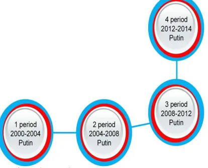
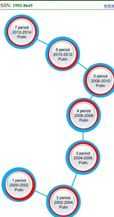
Figure 2 shows the similarity tree for the periods under review. The initial point, or the root of the similarity tree, is the class "1st_{period" (which}

includes audio fragments relating to the period from May 7, 2000 to May 7, 2004). The remaining classes are arranged such that the distance to each class is inversely proportional to the similarity value between this class and the class “1st_{period.” Thus,}

the greater the distance to the class is, the lower the similarity value is (between this class and the class

“1st_{period”), i.e., the method has defined these}

[image:5.612.316.523.493.660.2]

classes as less similar to each other.

Figure 2. Similarity Tree (Experiment 1)

(6)

5830 the most similar to the class “1st_{period” (the}

similarity value is equal to . . 0.97), then in decreasing similarity value order, classes "3rd

period" (the similarity value is equal to , .

0.86) and "4th_{period" (the similarity value is equal}

to . . 0.82) follow.

The numerical descriptors with the highest Fisher discriminant scores in this experiment (the most significant features in the process of the method) are: Histograms of fuzzy oriented gradients: 6.600000;

Multiscale histograms: 5.043756;

Combination of geometric moments: 4.252433; Radon transform features with the Chebyshev transform: 3.348936

Multiscale histograms with the Wavelet transform: 3.351107.

The sensitivity of the method was checked during the second experiment, when the input dataset was divided into shorter intervals. Seven two-year periods were taken for the experiment: May 7, 2000 – May 7, 2002;

May 7, 2002 – May 7, 2004;

May 7, 2004 – May 7, 2006; May 7, 2006 – May 7, 2008; May 7, 2008 – May 7, 2010; May 7, 2010 – May 7, 2012; May 7, 2012 – May 7, 2014.

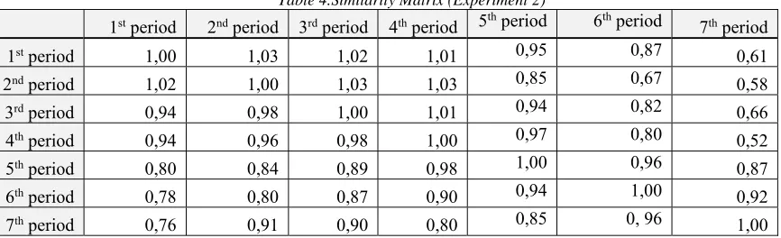
[image:6.612.92.525.451.583.2]

For each period, 18 audio fragments were taken, 14 of which were used for training with the remaining 4 for testing. Each of the audio records is a one-minute fragment from Vladimir Putin’s speeches. In each time interval, 7 audio fragments were taken from Vladimir Putin’s interviews where he answers journalists’ questions, and 11 fragments were from his prepared speeches beforehand. Like the first experiment, the second experiment was repeated 40 times with random allocation of the input audio files for training and test sets. The classification accuracy of a speech fragment to the correct time interval was 39%. One can notice that the accuracy has decreased in comparison with the previous experiment because of the reduction in the duration of the time intervals, and consequently there were less distinguished differences between them. Table 4 represents the similarity matrix of classes, computed as a result of the method’s work. Table 4.Sim

Table 4.Similarity Matrix (Experiment 2)

1st_period ₂nd_{period 3}rd_{period 4}th_{period 5}th period 6th period ₇th_period

1st_period _1,00 _1,03 _1,02 _1,01 0,95 0,87 _0,61

2nd_period _1,02 _1,00 _1,03 _1,03 0,85 0,67 _0,58

3rd_period _0,94 _0,98 _1,00 _1,01 0,94 0,82 _0,66

4th_period _0,94 _0,96 _0,98 _1,00 0,97 0,80 _0,52

5th_period _0,80 _0,84 _0,89 _0,98 1,00 0,96 _0,87

6th_period _0,78 _0,80 _0,87 _0,90 0,94 1,00 _0,92

(7)

[image:7.612.93.291.69.446.2]

5831 Figure 3. Similarity Tree (Experiment 2)

One can notice that the method was able to arrange the time periods in chronological order despite the decrease of the classification accuracy of the speech fragments to the correct time interval. Thus, the class “2nd_{period” is the most similar to the}

class “1st_{period” (the similarity value is equal to}

. .

1.025), then in decreasing similarity value order, the classes “3rd_{period” (the similarity}

value is equal to . . 0.98), “4th_{period” (the}

similarity value is equal to . . 0.975), “5th

period” (the similarity value is equal to . .

0.875), “6th_{period” (the similarity value is equal to}

. .

0.825) and finally “7th_{period” (the}

similarity value is equal to . . 0.685) follow.

The numerical descriptors with the highest Fisher discriminant scores in this experiment are:

Histograms of fuzzy oriented gradients: 5.846747;

Combination of geometric moments: 4.153543; Radon transform features with the Chebyshev transform: 3.564352;

Zernike Moments: 3.067110.

In another experiment, audio records of the speech of Barack Obama, the 44th_{President of The}

United States of America, were analysed, and the input dataset was split into four time intervals: January 20, 2007 – January 20, 2009;

January 20, 2009 – January 20, 2011; January 20, 2011 – January 20, 2013; January 20, 2013 – January 20, 2015.

Audio files for the experiment were downloaded from the website «www.americanrhetoric.com». For each period, 14 audio fragments were taken, 11 of which were used for training and the remaining 3 for testing. Each of the audio records is a one-minute fragment from Barak Obama’s interviews/speeches. The experiment was repeated 40 times with random allocation of the input audio files for training and test sets. The classification accuracy of speech fragments to the correct time intervals was 59%. Table 5 represents the similarity matrix of classes, computed as a result of the method’s work.

Table 5. Similarity Matrix (Experiment 3)

1st_period ₂nd_period ₃rd_period ₄th_period

1st_period _1,00 _1,00 _0,93 _0,93

2nd_period _0,97 _1,00 _0,98 _0,96

3rd_period _0,79 _0,80 _1,00 _0,96

[image:7.612.93.517.629.708.2]

(8)

5832 Figure 4 shows the similarity tree for the periods under review.

Figure 4. Similarity tree (Experiment 3)

Figure 4 shows that the method was able to arrange the time periods in chronological order. Thus, the class “2nd_{period” is the most similar to the}

class “1st_{period” (the similarity value is equal to}

. .

0.985), then in decreasing similarity value order, the classes “3rd_{period” (the similarity}

value is equal to . . 0.86) and “4th_period”

(the similarity value is equal to . . 0.8) follow.

Combination of geometric moments: 4.201858; Multiscale histograms: 4.199756;

Combination of geometric moments with the Wavelet transform: 3.506478;

Combination of geometric moments with the Chebyshev transform: 3.052345.

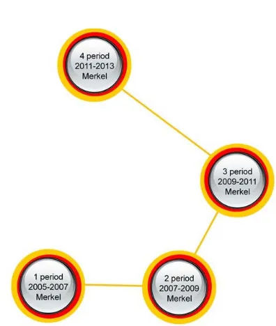
In another experiment, audio records with the speech of Angela Merkel, the Chancellor of Germany, were analysed, and the input dataset was split into four time intervals:

November 22, 2005 – November 22, 2007; November 22, 2007 – November 22, 2009; November 22, 2009 – November 22, 2011; November 22, 2011 – November 22, 2013.

Audio files for the experiment were downloaded from the official website of Bundestag «www.bundestag.de». For each period, 13 audio fragments were taken, 10 of which were used for training and the remaining 3 for testing. Each of the audio records is a one-minute fragment from one of Angela Merkel’s speeches. The experiment was repeated 40 times with random allocation of the input audio files for training and test sets. The method was able to classify an audio fragment to the correct period in 68% of cases. That is higher than the value of classification accuracy for any of the previous experiments. It means that, in the case of Angela Merkel, the speech characteristics have the most marked dynamics during the entire period under review (8 years – from November 22, 2005 to November 22, 2013). In addition, comparable results (65 %) were obtained in the case of Vladimir Putin when the input data were split into four periods lasting for 4, 4, 4 and 2 years – his first, second and third terms of his being the President of the Russian Federation and his term as The Chairman of the Government of the Russian Federation. Table 6 represents the similarity matrix of classes, computed as a result of the method’s work.

Table 6.Similarity Matrix (Experiment 4)

1st_period ₂nd_period ₃rd_period ₄th_period

1st_period _1,00 _1,02 _0,91 _0,69

2nd_period _0,86 _1,00 _0,89 _0,50

3rd_period _0,77 _0,91 _1,00 _0,58

[image:8.612.98.294.142.383.2]

(9)

5833 The classification accuracy of a speech fragment to the correct time interval can be increased by the preprocessing of the input data (including precorrection, or signal spectrum equalization, noise filtration, logarithmic spectrum compression, sound normalization).

Figure 5 shows the similarity tree for the periods under review. The figure shows that the method was able to arrange the time intervals in chronological order. As can be observed in Table 4, the class “2nd

period” is the most similar to the class “1st_period”

(the similarity value is equal to . . 0.94), then in decreasing similarity value order, the classes “3rd_{period” (the similarity value is equal to}

. .

0.84) and “4th_{period” (the similarity}

value is equal to . . 0.585) follow.

Combination of geometric moments: 8.985105; Multiscale histograms with the Wavelet transform: 8.310537;

[image:9.612.322.520.108.342.2]

Zernike Moments: 7.720533.

Figure 5. Similarity Tree (Experiment 4)

[image:9.612.94.523.580.714.2]

Also three extra experiments were carried out to show the generalization of the method. Audio records with the speeches of Jacques Chirac, George Bush and Vladimir Zhirinovsky were analysed. The input dataset was split into six time intervals for Jacques Chirac, four time intervals for George Bush and four time intervals for Vladimir Zhirinovsky. The summary information about the split and settings of the input data for these experiments is represented in Table 2. The classification accuracy of the method was 57%, 67% and 63% accordingly. The summary information about the experiments’ results is represented in Table 7. Table 7

Table 7.The Experiments’ Results Of Using The Automatic Method For Speech Analysis And Chronological Ordering

Experiment №

Speech fragments of politicians

Classification Accuracy

The ability to chronological ordering

1 Vladimir Putin 65% yes

2 Vladimir Putin 39% yes

3 Barak Obama 59% yes

4 Angela Merkel 68% yes

5 Jacques Chirac 57% yes

6 George Bush 67% yes

(10)

5834 4. DISCUSSION

In this research, the method operates with a feature set of 1030 features, which are numerical descriptors of the visual content of 460 spectrograms. After each of the numerical descriptors is assigned a Fisher discriminant score, 70% of the features with the lowest Fisher discriminant scores are discarded. The final set is 309 numerical descriptors. The similarity value between two time periods is determined by the average distance of all audio fragments in one period to all audio fragments in another period.

The experimental results showed that the proposed method was able to arrange the time intervals in chronological order, i.e., it was able to track the changes in the human speech characteristics, which had occurred during the certain period of time (in this research, periods lasting for 8-14 years were under review).

The changes in the human speech characteristics can be caused by a wide range of reasons. Probably, for the persons under review the main two are aging and changes in the style of speech and performance, connected with the strengthening of their politician’s positions or changing in the political situation in the state.

One can also notice, that the result of the method’s work doesn’t depend on the sex and age of the politician and the language, in what the samples were recorded.

The method’s sensitivity was also checked in a separate experiment in which the input dataset was divided into shorter intervals. The results showed that, even in this case, the method was able to arrange the time periods in chronological order despite the decrease of the classification accuracy of speech fragments to the correct time intervals. The similarity matrix of classes is visualized and represented as the similarity tree in the present research. In addition, the most significant features for the analysis of speech fragments were found: histograms of fuzzy oriented gradients, multiscale histograms, and combinations of geometric moments. However, the main disadvantage of the approach is processing time. Extracting the feature vector from a single spectrogram takes approximately 6 minutes (for a single Intel Core-i7 processor). In general, the experimental results show that the comprehensive morphological analysis of spectrograms can be effectively used for audio analysis.

5. CONCLUSION

Sound is a complex data type if it is considered in terms of automatic analysis via computing machines. In this paper, a method using the comprehensive morphological analysis of audio fragments’ spectrograms to produce the time periods’ similarity matrix was described.

The classification accuracy of speech fragments to the correct time intervals can be increased by the preprocessing of the input data (including precorrection or signal spectrum equalization, noise filtration, logarithmic spectrum compression, and sound normalization). The classification accuracy of the method can also be improved by increasing / reducing the size of the feature vector used for the analysis and by varying the duration of the audio fragments included in the experimental dataset. However, it should be remembered that increasing the feature vector size always results in the increase of the processing time.

Such methods can be very useful for the organization and chronological ordering of audio data (for example, to create audio archives automatically), as well as for the analysis and visualization of speech characteristic similarities, which can be used in such research as a person's identification by voice and the detection of similar voices.

REFRENCES:

[1] Y. Panagakis, C. Kotropoulos, and G. R. Arce, “Non-Negative Multilinear Principal Component Analysis of Auditory Temporal Modulations for Music Genre Classification”,

IEEE Transsaction on Audio, Speech and

Language Processing, Vol. 18, No. 3, 2010, pp.

576–588.

[2] K. Chang, J. Jang, and C. Lliopoulos, “Genre Classification via Compressive Sampling”,

Proceedings of International Society for Music Information Retrieval Conference Music Genre

Classification via Compressive Sampling, 2010,

pp. 387–392.

[3] Y. Kim, E. Schmidt, R. Migneco, B. Morton, P. Richardson, J. Scott, J. Speck, and D. Turnb, “Music Emotion Recognition: A State of the Art Review”, Proceeding of International Society for Music Information Retrieval Conference Music Genre Classification via Compressive

Sampling, 2010, pp. 255–266.

(11)

5835

Transsaction on Audio, Speech and Language

Processing, Vol. 21, No. 4, 2013, pp. 737–748.

[5] B. Mcfee, L. Barrington, and G. Lanckriet, “Learning Content Similarity for Music Recommendation”, IEEE Transsaction on

Audio, Speech and Language Processing, Vol.

20, No. 8, 2012, pp. 2207-2218.

[6] J. Serra, H. Kantz, X. Serra, and R. Andrzejak, “Predictability of Music Descriptor Time Series and its Application to Cover Song Detection”,

IEEE Transsaction on Audio, Speech and

Language Processing, Vol. 20, No. 2, 2011, pp.

514–525.

[7] A. Manders, D. Simpson, and S. Bell, “Objective Prediction of the Sound Quality of Music Processed by an Adaptive Feedback Canceller”, IEEE Transsaction on Audio,

Speech and Language Processing, Vol. 20, No.

6,2012, pp. 1734–1745.

[8] E. G. Vidal, E. F. Zarricueta, and F. A. Cheein, “Human-inspired sound environment recognition system for assistive vehicles”,

Journal of Neural Engineering, Vol. 12, No. 1,

2015.

[9] X. Song, B. Wallace, J. Gardner, N. Ledbetter, K. Weinberger, and D. Barbour, “Fast, Continuous Audiogram Estimation Using Machine Learning”, Ear and Hear, Vol. 36, No.

6, 2015, pp. 326-335.

[10] Y.P. Huang, S.L. Lai, and F.E. Sandnes, “A repeating pattern based Query-by-Humming fuzzy system for polyphonic melody retrieval”,

Applied Soft Computing, Vol. 33, 2015, pp.

197–206.

[11] M. Kaminskas, and F. Ricci, “Contextual music information retrieval and recommendation: State of the art and challenges”, Computer

Science Review, Vol. 6, No. 2, 2012, pp. 89–

119.

[12] Z. Fu, G. Lu, K. Ting, and D. Zhang, “A Survey of Audio-Based Music Classification and Annotation”, IEEE Transaction on Multimedia,

Vol. 13, No. 2, 2011, pp. 303–319.

[13] J. George and L. Shamir, “Computer analysis of similarities between albums in popular music”,

Patter Recognition Letters, Vol. 45, No. 1,

2014, pp. 78-84.

[14] Y. Costa, L. Oliveira, and A. Koerich, “Music genre recognition using spectrograms”,

Proceeding of International Conference on

Systems, Signals and Image, 2011, pp. 1–4.

[15] B. Ghoraani, and S. Krishnan, “Time– Frequency Matrix Feature Extraction and Classification of Environmental Audio Signals”, IEEE Transsaction on Audio, Speech

and Language Processing, Vol. 19, No. 7,

2011, pp. 2197–2209.

[16] Y. Costa, L. Oliveira, A. Koerich, F. Gouyon, and J. Martins, “Music genre classification using LBP textural features”, Signal

Processing, Vol. 92, No. 11, 2012, pp. 2723–

2737.

[17] L. Shamir, “Computer Analysis Reveals Similarities between the Artistic Styles of Van Gogh and Pollock”, Leonardo, Vol. 45, No. 2,

2012, pp. 149–154.

[18] L. Shamir and J. Tarakhovsky, “Computer analysis of art”, Journal on Computing and

Cultural Heritage, Vol. 5, No. 2, 2012, pp. 1–

11.

[19] S. Biswas and A. Biswas, “Face Recognition Algorithms based on Transformed Shape Features”, IJCSI International Journal of

Computer Science, Vol. 9, No. 3, 2012, pp. 445–

451.

[20] M. Yang, L. Zhang, S. Shiu, and D. Zhang, “Gabor feature based robust representation and classification for face recognition with Gabor occlusion dictionary”, Pattern Recognition,

Vol. 46, No. 7, 2013, pp. 1865–1878.

[21] C. Adak, “Gabor Filter and Rough Clustering Based Edge Detection”, Proceeding of International Conference on Human Computer

Interactions, 2014,pp. 1–5.

[22] J. Feng, B. Ni, D. Xu, and S. Yan, “Histogram Contextualization”, IEEE Transactions on

Image Processing, Vol. 21, No. 2, 2012, pp.

778–788.

[23] A. Shaikh, D. Kumar, and J. Gubbi, “Automatic visual speech segmentation and recognition using directional motion history images and Zernike moments”, Visual Computer, Vol. 29,

No. 10, 2013, pp. 969–982.

[24] A. Iosifidis, A. Tefas, N. Nikolaidis, and I. Pitas, “Multi-view human movement recognition based on fuzzy distances and linear discriminant

analysis”, Computer Visual Image

Understanding, Vol. 116, No. 3, 2012, pp. 347–

360.

[25] M. Hickman, “Geometric Moments and Their Invariants”, Journal of Mathematical Imaging

and Visions, Vol. 44, No. 3, 2012, pp. 223–235.

[26] Z. Ji, Y. Xia, Q. Sun, Q. Chen, and D. Feng, “Adaptive scale fuzzy local Gaussian mixture model for brain MR image segmentation”,

Neurocomputing, Vol. 134, 2014, pp. 60–69.

(12)

5836 Distribution”, Journal of Machine Learning Research, Vol. 15, 2014, pp. 3743–3773. [28] S. Jain, A. Jain, S. Verma, S. Susan, and A.

Sharma, “Fuzzy match index for scale-invariant feature transform (SIFT) features with application to face recognition with weak supervision”, IET Image Processing, Vol. 9,

No. 11, 2015, pp. 951–958.

[29] A. Salhi, M. Kardouchi, and N. Belacel, “Histograms of fuzzy oriented gradients for face recognition”, Proceeding of 2013 International Conference on Computer Applications

Technology (ICCAT), 2013, pp. 1–5.

[30] W. El-Tarhouni, M. Shaikh, L. Boubchir, and A. Bouridane, “Multi-scale shift local binary pattern based-descriptor for finger-knuckle-print recognition”, Proceeding of 2014 26th International Conference on Microelectronics

(ICM), 2014, pp. 184–187.

[31] A. Gilbert, P. Indyk, M. Iwen, and L. Schmidt, “Recent Developments in the Sparse Fourier Transform: A compressed Fourier transform for big data”, IEEE Signal Processing Magazine, Vol. 31, No. 5, 2014, pp. 91–100.

[32] T. Backstrom, C. Pedersen, J. Fischer, and G. Pietrzyk, “Finding line spectral frequencies using the fast fourier transform”, Proceeding of 2015 IEEE International Conference on Acoustics, Speech and Signal Processing

(ICASSP), 2015, pp. 5122–5126.

[33] S. Du, D. Huang, and J. Lv, “Recognition of concurrent control chart patterns using wavelet transform decomposition and multiclass support vector machines”, Computers & Industrial

Engineering, Vol. 66, No. 4, 2013, pp. 683–

695.

[34] M. Subrahmanyam, R. Maheshwari, and R. Balasubramanian, “Local maximum edge binary patterns: A new descriptor for image retrieval and object tracking”, Signal

Processing, Vol. 92, No. 6, 2012, pp. 1467–