ISSN 2286-4822 www.euacademic.org
Impact Factor: 3.1 (UIF)
DRJI Value: 5.9 (B+)
Surface Water Modeling Using SCS-CN Model
-Hydroinformatic Approach
ASHENAFI TOLESSA GURMU G. ASHENAFI TOLESSA
Lecturer, Adama Science and Technology University Adama, Ethiopia
Abstract:
Tandava River Basin experiencing undeterministic flood, overflow in the reservoir and soil erosion due to surface runoff. This study aiming to blend the application of Remote Sensing (RS) and Geographic Information System (GIS) techniques to estimate surface runoff based on the land use/land cover, hydrological soil group, rainfall data (P), Potential Maximum Retention (S), Antecedent Moisture Condition (AMC), and Weighted Curve Number (CN). Soil Conservation Service (SCS) model is used for surface runoff estimation. The data for the above mention parameters are acquires from different governmental offices and all SCS model parameters are derived by using remote sensing and GIS techniques. From middle of June to October, the river basin as a whole and the remaining sub-basins generated considerable amount of runoff because of monsoon season rainfall in these regions. During June to October, in most of the basins, around 90% of annual runoff occurred except in the sub-basin 1, 7 and 17.therefore such model helps to estimate surface runoff and support to take flood prevention measures, soil conservation action and Check dam recommendation.
Introduction
The information access and accuracy has lion portion to get good result on runoff estimation in which in India this is scarce. However, to see and highlight basin management programme for conservation and development of natural resource and its management, the runoff information assumes great relevance. Runoff model is best expressed by spatially variable parameters such as rainfall, soil types and land use / land cover etc. (Kumar, 1997).
The development of geographic information system (GIS) and remote sensing techniques, the hydrological catchments models have been more physically based and distributed to enumerate various interactive hydrological processes considering spatial heterogeneity (Mohan and Shrestha 2000).
Study area
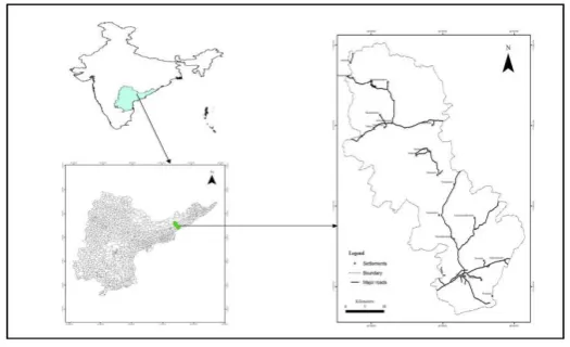
The study area, Tandava River Basin, is bounded in between North latitudes 17020’ to 17050`N and East longitudes 82020` to
82040’ E. It forms part of Survey of India Toposheets 65 K/5,
K/6, K/7, K/10 and K/11 and covers an area of 1283 Km2. Major
part of the area is in Visakhapatnam district but adjacent drainage carries under the jurisdriction part of East Godavari district is also included to see the total Morphometric of the drainage basin (figure 1.1).
Figure 1.1: Location map of the study area
Methodology
Rainfall
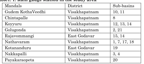
Table1. 1: Rain gauge station in the study area
Mandals District Sub-basins
Gudem KothaVeedhi Visakhapatnam 10, 11
Chintapalle Visakhapatnam 8
Koyyuru Visakhapatnam 12, 13, 14
Golugonda Visakhapatnam 2, 21
Rajavommangi East Godavar 15, 14
Nathavaram Visakhapatnam 1, 7, 17, 18
Kotananduru East Godavar 19
Nakkapalli Visakhapatnam 3, 4
Payakaraopeta Visakhapatnam 20
Normals of Rainfall Data
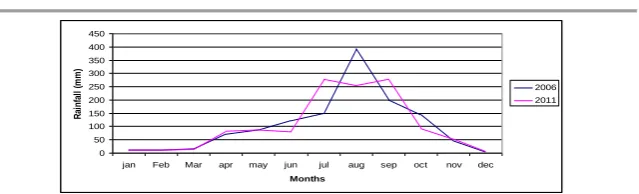
The length or period of record needed to achieve stability varies between seasons and regions. Based on World Meteorological Organization (WMO) rainfall data of 30 years is adequate under Indian conditions. For this study, the current normal period is 2006-2011.
Figure 1.2: Monthly normal rainfall distribution
Determination of Average Rainfall
According to litratures (MWRI, 2007), in this study we apply arithmetic mean method in order to determine average depth of rainfall of the drainage basin.
Where, P is the average rainfall, n, the number of years of data and P1, P2, P3 ……… Pn , precipitations measured at stations 1, 2,3 ……… n.
The total depth of the rainfall for the study period is (2006 total + 2011total) / 2 = 774mm.
Rainfall Frequency curve
In this graph the peak rainfall for the time span of 5 years is 774mm. It occurs with a time interval of 56 months. For 65 months, the probable rainfall estimated is 660mm.
Pro = m * 100 1.2
N+1
Where Pro- Probability percent of peak rainfall m - Ranking of the storm
N – No. of months
0 50 100 150 200 250 300 350
0 20 40 60 80 100
Probability (%)
R
ai
nf
al
l
(m
m
)
Figure 1.3: Rainfall frequency Curve
T =100/Pro 1.3 Where T – recurrence time interval
0 50 100 150 200 250 300 350 400 450
jan Feb Mar apr may jun jul aug sep oct nov dec
Months R ai nf al l (m m ) 2006 2011
Figure 1.4: Average mean monthly rainfall correlation between 2006 Vs 2011
Soils
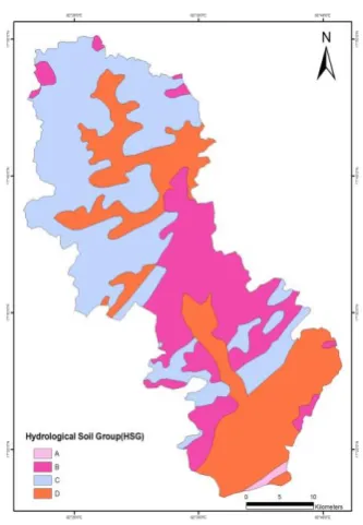
Figure 1.5: Soil map of the study area, based on Visakhapatnam and East Godavari soil sheets
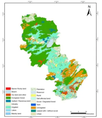
Land use
Land use/land cover is one of the very important variables for runoff estimation. Visual interpretation cross checked and verified by ground truth data is used to classify both LANDSAT-7 and IRS-P6 LISS III satellite data using ArcGIS software. After field verification, initial classification is modified by recoding techniques and final land use/land cover map is produced (Fig. 1.6-1.7). The detail statistics of land use/land cover of the study area is shown in table 1.2.
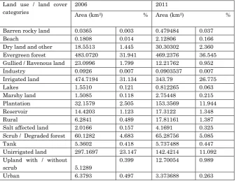
Table 1.2: Statistical data of land use land cover Land use / land cover
categories
2006 2011
Area (km2) % Area (km2) %
Barren rocky land 0.0365 0.003 0.479484 0.037
Beach 0.1808 0.014 2.12806 0.166
Dry land and other 18.5513 1.445 30.30302 2.360 Evergreen forest 483.0720 31.941 469.2376 36.545 Gullied / Ravenous land 23.0996 1.799 12.21762 0.952
Industry 0.0926 0.007 0.0903537 0.007
Irrigated land 474.7194 31.134 343.79 26.775
Lakes 1.5510 0.121 0.812265 0.063
Marshy land 1.5085 0.118 2.75448 0.215
Plantation 32.1579 2.505 153.3569 11.944
Reservoir 14.4203 1.123 17.3122 1.348
Rural 6.2841 0.489 17.81161 1.387
Salt affected land 2.0166 0.157 4.1691 0.325
Scrub / Degraded forest 60.1282 4.683 65.28756 5.085
Tank 5.3602 0.418 5.737488 0.447
Unirrigated land 297.1697 23.147 142.4214 11.092 Upland with / without
scrub 5.1289
0.399 12.70054 0.989
Figure 1.6: Land use/ land cover map generated from Landsat TM scene, 2006 of the study area
Antecedent Moisture Condition (AMC)
AMC refers to the moisture content present in the soil at the beginning of the rainfall-runoff event under consideration. It is well known that initial abstraction and infiltration and are governed by AMC. For purposes of practical application three level of AMC are recognized by SCS as follows:
AMC-I: Soils are dry but not to wilting point. Satisfactory cultivation has taken place.
AMC-II: Average conditions
AMC-III: Sufficient rainfall has occurred within the immediate past five days. Saturated soil conditions prevail.
Table 1.3: Antecedent moisture conditions (AMC) for determining the values of CN
AMC Type Total rain in previous 5 days
Dormant season Growing season
I Less than 13 mm Less than 36 mm
II 13 to 28 mm 36 to 53 mm
III More than 28 mm More than 53 mm
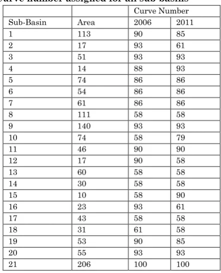
Curve number estimation
land use information by using logical expression. The weighted curve number for each sub basin is calculated by using the Equation 1.4.
Table 5.7: Curve number assigned for all sub-basins Curve Number
Sub-Basin Area 2006 2011
1 113 90 85
2 17 93 61
3 51 93 93
4 14 88 93
5 74 86 86
6 54 86 86
7 61 86 86
8 111 58 58
9 140 93 93
10 74 58 79
11 46 90 90
12 17 90 58
13 60 58 58
14 30 58 58
15 10 58 90
16 23 93 61
17 43 58 58
18 31 61 58
19 53 90 85
20 55 93 93
21 206 100 100
Weighted CN= CN1x A1 + CN2x A2 + CN3x A3---CNnXn (1.4)
A1 + A2---An
Where,
CN1, CN2, --- CNn are the curve numbers for different land uses
and treatment, and hydrologic soil groups present in the sub-basin of the total river basin
A1, A2, ---An. are its respective sub-basin areas.
Rainfall –Runoff calculations are done for each sub-basin. The quality of this model is improved by incorporating the spatial variation of watershed characteristics using Remote Sensing and GIS. The runoff curve numbers (AMC II) for hydrologic soil cover complexes and curve number adjustments for antecedent soil moisture conditions for Indian conditions are chosen from the information presented in the Handbook of Hydrology (1972).
The CN values arrived at based on the combination of land use and Hydrologic soil group are meant for AMC-II condition. CN values for AMC-I and AMC-III conditions have been calculated using conversion equations 1.5 and 1.6 given below.
CN1 = CN2 / 2.281 – 0.01281 .2CN2 (1.5)
CN3 = CN2 / 0.427 + 0.00573CN2 (1.6)
The values for the weighted CN as per AMCs were 68, 83 and 92 in 2006, 69, 84 and 92 in 2011 for the AMC I, II, and III, respectively.
Surface runoff estimation
The SCS-CN method is based on the water balance equation and two fundamental hypotheses. The first hypothesis equates the ratio of the amount of direct surface runoff Q to the total rainfall P (or maximum potential surface to the runoff) with the ratio of the amount of infiltration Fc amount of the potential
maximum retention S. The second to the potential hypothesis relates the initial abstraction Ia maximum retention. Thus, the SCS-CN method consisted of the following equations (Subramanya K. (2008).
(b) Ia - S hypothesis:
Ia=λS (1.9)
Where,
P is the total rainfall, Ia the initial abstraction, Fc the
cumulative infiltration excluding Ia, Q the direct runoff, S the potential maximum retention or infiltration and λ the regional parameter dependent on geologic and climatic factors (0.1<λ<0.3).
Solving equation (1.8)
Q = ( P −Ia)2 / 𝑃−𝐼𝑎+𝑆 (1.10)
Q = ( P−λS )2 / 𝑃− (λ−1) S (1.11)
The relation between Ia and S was developed by analyzing the rainfall and runoff data from experimental small watersheds and is expressed for Indian condition as Ia=0.3S. Combining the water balance equation and proportional equality hypothesis, the SCS-CN method is represented as
Q = (𝑃−0.3𝑆)2 / 𝑃+0.7𝑆 (1.12)
The potential maximum retention storage S of watershed is related to a CN, which is a function of land use, land treatments, soil type and antecedent moisture condition of watershed. The CN is dimensionless and its value varies from 0 to 100.The S-value in mm can be obtained from CN by using the relationship
Results and Discussions
The result shows that considerable amount of runoff from rainfall. The sub-basin wise average CN was found to be the lowest fifty eight (58) for the sub-basin 8, 10, 12, 13, 14, 15, 17 and 18, the reason being good vegetation. But runoff potential was high in the sub-basin 8, 10, 12, 13, 14, 15, 17 and 18 because of AMC III condition during most of the months. As assigned CNs were based on average AMC II condition, CNs were later modified for AMC I (rainfall < 5 mm), and AMC III (rainfall > 71 mm) conditions. High CNs in the sub-basin 2, 3, 4, 9, 16, and 20 ninety three (93) were due to dominant HSG-C. CN for the remaining sub-basins ranges between 85 and 61.
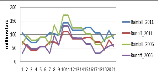
It was observed that only the sub-basins 10 and 11 generated considerable amount of runoff throughout the study period, because the sub-basins received rainfall between 1587.4 and 1317.67 millimeter during 2006 and 2011. From middle of June to October, the river basin as a whole and the remaining sub-basins generated considerable amount of runoff because of monsoon season rainfall in these regions. During June to October, in most of the sub-basins, around 90% of annual runoff occurred except in the sub-basin 1, 7 and 17. The runoff pattern from June to September typically matched with the advancement of the monsoon system.
runoff was observed between January and February, though peak runoff was almost reduced by two-thirds. Sub-basin 1, 2, 3, 4, 5, 6 and 21 had low runoff throughout the year. Thus the spatial variability of runoff was high during five months, i.e. June to September. During other months, there was low spatial variability of runoff, because most of the sub-basins had low rainfall.
The spatial variation of annual runoff showed high runoff (1587.44–1317.67 millimeter) in the sub-basins 10, 11 and 12 due to high annual rainfall in these regions (2056.8– 1717.6 millimeter). Low to very low runoff depth of the order 368.83– 682.58 millimeter was observed in sub-basins 1, 2, 3, 4, 5, 6, 7, 8, 17, 18, 19, 20 and 21, caused by low to very low rainfall (754–1026.1 millimeter). Medium to high runoff 1033– 1051 millimeter was found in the sub-basins 9, 13, 14, 15 and 16. The average annual runoff depth over Tandava River Basin was found to be 819.27 millimeter, which was around 66.8% of the total rainfall in Tandava River Basin, i.e. 1225.75 millimeter. Though the runoff pattern mostly followed the rainfall pattern, there were deviations, that could be attributed to variation in textural classes and hydrological land cover classification generated using remote sensing
Conclusions and recommendations
The SCS-CN model provides a very sufficient solution for this study interms of estimating surface runoff from two rainfall year that is 2006 and 2011 and hence the researcher recommend this valuable document for the safeguard of the Tandava River Basin community for further prevention, mitigation and conservations activity that cause due to excess rainfall occurrence. These results also recommend further extension work of the current reservoir in order to prevent abrupt flood and built of check dams in the upper catchment of the river basin.
Acknowledgments
This paper may not be come into fulfillment without the strong encouragement and support of my dearest wife Fiker ( Rahel T. Tadesse). Thanks, my dear Fiker!
REFERENCES
Arwa D. O. (2001) GIS Based Rainfall Runoff Model for the Turasha Sub Catchment Kenya, MSc. thesis. International institute for aero space survey and earth sciences, Enschede, the Netherlands.
Kumar P, Tiwari KN and Paul DK (1997) Establishing SCS runoff curve number from IRS digital database. J. Indian Soc. Remote Sensing, 19, 246-251.
McCuen RH. 1982. A Guide to Hydrologic Analysis Using SCS Methods. Prentice-Hall: Englewood Cliffs, NJ.
due to Land use modifications, proceeding of symposium on Restoration of Lakes and Wetlands, Indian Institute of Science, November 27-29, 2000, Banglore, India. SCS, Soil Conservation Department, “Handbook of Hydrology”,
Ministry of Agriculture, New Delhi, 1972.
Soil Conservation Service (1972) Hydrology. National Engineering Hand book, Sec.4, U.S. Govt. Printing office, Washington D.C.