Spectrum Relation of Linear MIMO Structures in Short
Range Imaging
Xiaozhou Shang, Jing Yang, and Zhiping Li*
Abstract—This paper discusses the spectrum relation in Multiple-Input-Multiple-Output (MIMO)
structures and presents an imaging algorithm for sparse linear MIMO array for short range imaging. This algorithm is available for MIMO array consisted by transmit and receive arrays separated from each other. The wave propagation process is used to interpret the spectrum relation in linear MIMO structures; therefore, the convolution relation of spectrum can be clearly understood. Moreover, the spectrum shift effect in linear MIMO structure with separated transmit and receive arrays is discussed and solved according to the spectrum relation. Above all, the imaging algorithm for sparse linear MIMO structure is presented, and the image performance is demonstrated by simulation results.
1. INTRODUCTION
In surveillance and security applications, high resolution imaging radar systems in millimeter and terahertz bandwidth are demanded due to the penetrating properties of the EM wave [1]. The high resolution requirement indicates a large size of aperture array, which is difficult to be realized by phased arrays because of the hardware cost. Moreover, the imaging speed requirement is also difficult to be fulfilled by using synthetic aperture. However, Multiple-Input-Multiple-Output (MIMO) technique presents an outstanding solution by forming a large virtue array simultaneously through signal processing with only few transmit and receive channels. Therefore, high resolution MIMO imaging systems are rapidly developed in current surveillance and security territories [2–4].
Performance of MIMO imaging radar can be easily understood from its virtue array, since the pattern of a MIMO structure is the multiplexed result of its transmit and receive array patterns [5]. However, this relation only stands under the far field assumption. For short range situations, to acquire a well focused high resolution image, the near-field problem cannot be ignored. The generalized Back Projection (BP) is available for arbitrary imaging structures, but cost lots of computation resources. Alternatively, spectrum domain algorithms like Range Migration Algorithm(RMA) is available for near-field situations. The RMA [6] solves the wave propagation relation in spatial spectrum domain with no near-field approximations and is very efficient for computation by taking the advantage of Fast Fourier Transform(FFT). Although RMA has been introduced for MIMO or other similar structures in many articles, it was processed on the MIMO virtue array [7, 8] or still took approximations and got an inaccurate description of spectrum [9]. Thus the spectrum relation in MIMO structure is not clearly revealed.
In our previous work [10], the convolution relation of spectrum in MIMO structure is provided and used to design the imaging algorithm for sparse linear MIMO array. In this paper, the spectrum relation in MIMO structure is well interpreted with the wave propagation process. This relation is used to design imaging algorithm for the general cases of sparse linear MIMO array, which consists
Received 9 January 2018, Accepted 14 March 2018, Scheduled 11 April 2018
* Corresponding author: Zhiping Li (zhiping [email protected]).
of dense and sparse arrays separated from each other, as in [2, 3]. The next paragraphs are organized as following: Section 2 provides the spectrum relation in MIMO structure, and imaging algorithm for sparse linear MIMO array is proposed in Section 3. Section 4 gives the implementation and simulation result for the proposed algorithm, and all the methods are concluded in Section 5.
2. MIMO SPECTRUM ANALYZE
Considering a general case of a linear MIMO array consisting of a transmit and a receive array with evenly spaced antennas. The signal is emitted from the transmitter and echoed by the target then collected by the receiver, as shown in Fig. 1.
Figure 1. Linear MIMO imaging scene.
After match-filtering, the data are separated to each specified transmitter-receiver pair, and only propagation phase term is preserved while the amplitude is determined by the reflectivity of the target, as expressed below:
R(xt, xr, k) =
s(x0, y0)e−jk √
(xt−x0)2+(y0+d)2+√(xr−x0)2+(y0+d)2
dx0dy0 (1)
HereR(xt, xr, k) indicates the data by transmitter and receiver positioned atxtand xr, respectively;k is the wave number;s(x0, y0) is the reflectivity map of the target object. The two square root terms on the exponential part are the propagation range of transmit and receive paths respectively.
To reveal the spectrum relation in the MIMO array, Fourier Transform (FT) is taken on both transmitter and receiver dimensions to transform into spectrum domain:
R(kxt, kxr, k) =
s(x0, y0)
e−jk √
(xt−x0)2+(y0+d)2e−jkxtxtdx t
e−jk √
(xr−x0)2+(y0+d)2e−jkxrxrdx r
dx0dy0 (2)
The two inner integrals can be calculated by the Method of Stationary Phase (MSP) and result in:
R(kxt, kxr, k) =
s(x0, y0)e−jkxx0e−jky(y0+d)dx0dy0 (3)
where:
kx =kxt+kxr, ky =
k2−k2 xt+
k2−k2
The right side of Equation (3) forms a FT expression; however, the FT relation stands for (kx and ky), thus the spectrum expression at left must be firstly projected to R0(kx, ky). To clearly interpret the spectrum relation, the MSP theory must be examined since the spectrum expression is calculated from it.
The MSP theory suggests that only the neighbor value of the stationary point mainly contributes to the integral. Therefore, the stationary point determines the effective spectrum which is collected in the received data:
kxt =k
xt−x0
(xt−x0)2+ (y0+d)2
, kxr =k
xr−x0
(xr−x0)2+ (y0+d)2
(5)
Equation (5) indicates that the phase propagation coefficient of x0 is ksinθ1+ksinθ2. According to Equation (4), the coefficient of y0 is kcosθ1 +kcosθ2, and the definition of θ1 and θ2 can be seen in Fig. 1. As a result, the effective spectrum of a specified target point collected by a specified transmitter-receiver is a plane wave propagates with direction θ1 then refracted to direction θ2. It is worth to note that the near-field situation in short range imaging is referenced to the MIMO array, but any transmit-receive antenna pairs work in the far-field situation, which also supports the plane wave propagation conclusion.
Consider that the transmit and receive arrays of the MIMO structure are all centered at the original point as a simplified situation. According to the above relations, the spectrum of two different point targets in the same sparse linear MIMO structure can be calculated, shown in Fig. 2, and the different colors in the spectrum correspond to different transmitters.
-0.2 0 0.2 0.4 0.6 0.8 1 1.2 1.4
Range (m) -0.5
-0.4 -0.3 -0.2 -0.1 0 0.1 0.2 0.3 0.4 0.5
A
z
im
ut
h (
m
)
Imaging scene
Transmitter Receiver Target point
800 900 1000 1100 1200 1300
ky -300
-200 -100 0 100 200 300
kx
spectrum of target at center
800 900 1000 1100 1200 1300
ky -300
-200 -100 0 100 200 300
kx
spectrum of target at side
(a) (b) (c)
Figure 2. Spectrum of target points in MIMO structure. (a) Imaging scene. (b) Spectrum of point at
target center. (c) Spectrum of point away from target center.
It is clear to see that for a sparse transmit array with a dense receiver array, the main effects of the transmitters are illuminating the different parts of the total spectrum. Moreover, for target points at different positions, their spectrums distribute in different regions. As a result, for a distributed target, the parts of spectrum corresponding to different transmitters must be added together to form the total spectrum. Mathematically, this process is expressed as:
R0(kx, ky) =
R(kxt, kx−kxt, ky)dkxt (6)
target is a 2-D matrix. Equation (6) provides an integration on the 3-D spectrum of data then lowers it to 2-D to match the target spectrum. It is worth to note that to complete this integral, phase compensating of e−jkyd should be firstly completed since the value ofk
y is determined by bothkxt and
kxr. Then the Stolt interpolation should be processed to projectR(kxt, kxr, k) toR(kxt, kxr, ky). After these two steps, this integral can be calculated correctly, taking FT to transform the spectrum back to space domain.
3. IMAGING ALGORITHM FOR SPARSE LINEAR MIMO ARRAYS
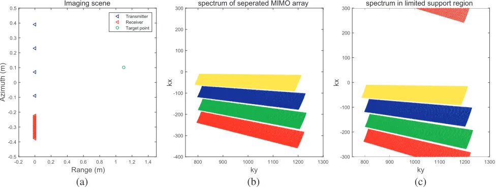
For the general case of sparse linear MIMO arrays, the transmitter and receiver arrays are not all centered at the original point. According to the presented spectrum relation, the target spectrum will also be shifted, as shown in Fig. 3.
-0.2 0 0.2 0.4 0.6 0.8 1 1.2 1.4
Range (m) -0.5
-0.4 -0.3 -0.2 -0.1 0 0.1 0.2 0.3 0.4 0.5
Azimut
h (m)
Imaging scene
Transmitter Receiver Target point
800 900 1000 1100 1200 1300
ky -400
-300 -200 -100 0 100 200 300
kx
spectrum of seperated MIMO array
800 900 1000 1100 1200 1300
ky -300
-200 -100 0 100 200 300
kx
spectrum in limited support region
(a) (b) (c)
Figure 3. Spectrum in separated MIMO array. (a) Imaging scene. (b) Spectrum of target point. (c)
Spectrum of target point in limited support region.
If the center shift values of transmitter and receiver arrays arext c andxr c, respectively, Equation (3) can be rewritten as:
R(kxt, kxr, k) =
s(x0, y0)e−jkxx0e−jky(y0+d)ej(kxtxt c+kxrxr c)dx0dy0 (7)
The arrays’ shift causes phase term to be expressed as the third exponential term in Equation (7), which needs to be compensated.
However, the MIMO image cannot be correctly obtained if only the additional phase term is compensated. Since the spectrum support region is determined by the element interval of the array, the target spectrum shifts in the support region and may be convolved, as shown in Fig. 3(c). Although taking the Nyquist sampling rate λ/2 avoids this problem, in practical cases, it is difficult to realize this requirement, and only sampling rate satisfying no aliasing in the Field of View (FOV) is used. Therefore, the convolved spectrum must be shifted back to ensure correct phase compensating and Stolt interpolating processes. According to the theory of discrete Fourier transform, shift in spectrum domain can be realized by phase multiplexing in space domain. Therefore, spectrum shift can be completed by phase multiplexing with the original MIMO data R(xt, xr, k) in space domain, and the multiplexed phase term is:
ϕ(xt, xr, k) =e−jxtkxt c/
√
x2t c+d2e−jxrkxr c/√x2r c+d2 (8)
(kx, ky) is expected for FFT, Stolt interpolation is taken to projectkto ky grid. Moreover, for variable kx, same grid size ofkxt andkxr is expected to avoid additional interpolation processes. Therefore, zero-inserting and zero-padding on sparse transmit array and dense receive array are demanded, respectively, or vice versa. By expanding the space domain data onto the same size of space grid, the spectrum grid size will also be the same according to FT performance. This process is very important not only to avoid additional interpolation demand but also to avoid aliasing problems. Zero-inserting on sparse array expands the region ofkxt to a correct value as in Equation (5), and zero-padding on dense array expands the non-aliasing area of the final image since the dense array is always a short array.
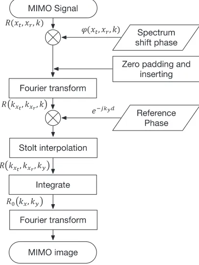
A flowchart of the imaging algorithm for sparse linear MIMO array is organized in Fig. 4.
Figure 4. Flow chart of imaging algorithm.
The original signal is firstly multiplied with the phase term in Equation (8) to shift the spectrum to center position, then takes zero-inserting and zero-padding to satisfy the proper spectrum grid. After Fourier transform, the spectrum domain data are compensated with the propagation phase term, and Stolt interpolation is processed. The total spectrum of target is achieved through the integrating in Equation (6), and the final image can be obtained by transforming the spectrum into space domain.
4. SIMULATION AND IMAGE PERFORMANCE
To validate the proposed algorithm, simulation is performed by coding in Matlab. The MIMO imaging array is composed by a sparse transmit array and a dense receive array both with 8 elements. The transmit array is centered at −0.15 m with 0.08 m element interval, and the receive array is centered at 0.3 m with 0.01 m interval, respectively. The target consists of 3∗3 evenly spaced points with 0.2 m interval in both range and azimuth. The working frequency band is in Ka band from 30 GHz to 40 GHz, and the sketch of the imaging scene is shown in Fig. 5(a).
-0.2 0 0.2 0.4 0.6 0.8 1 1.2 1.4 Range (m) -0.6 -0.4 -0.2 0 0.2 0.4 0.6 A z im ut h ( m ) Imaging scene Transmitter Receiver Target point Recovered spectrum
1100 1200 1300 1400 1500 1600
ky -300 -200 -100 0 100 200 300 kx Imaging result
0.5 0.6 0.7 0.8 0.9 1 1.1 1.2 1.3 1.4 1.5
Range (m) -0.5 -0.4 -0.3 -0.2 -0.1 0 0.1 0.2 0.3 0.4 0.5 A z im ut h (m ) -30 -25 -20 -15 -10 -5 0
(a) (b) (c)
Figure 5. Simulation results. (a) Imaging Scene. (b) Recovered target spectrum. (c) Target image.
Imaging by BP method
0.5 0.6 0.7 0.8 0.9 1 1.1 1.2 1.3 1.4 1.5
Range (m) -0.5 -0.4 -0.3 -0.2 -0.1 0 0.1 0.2 0.3 0.4 0.5 A z imuth (m ) -30 -25 -20 -15 -10 -5 0
Imaging by EPC method
0.7 0.8 0.9 1 1.1 1.2 1.3
Range (m) -0.5 -0.4 -0.3 -0.2 -0.1 0 0.1 0.2 0.3 0.4 0.5 Azi m u th (m) -30 -25 -20 -15 -10 -5 0 Imaging result
0.5 0.6 0.7 0.8 0.9 1 1.1 1.2 1.3 1.4 1.5
Range (m) -0.5 -0.4 -0.3 -0.2 -0.1 0 0.1 0.2 0.3 0.4 0.5 A z im ut h ( m ) -30 -25 -20 -15 -10 -5 0
(a) (b) (c)
Figure 6. Imaging result by (a) BP method, (b) EPC method, (c) the proposed method.
in dB form, and the dynamic range is set to 30 dB. All 9 target points are correctly focused even for point far away from target center, which confirms that the algorithm is available for large scene in short range imaging. Although side lobes of target points closer to the MIMO array affect each other, the interacted side lobe levels are all smaller than−15 dB. Moreover, the side lobe trajectories of all target points clearly reveal the different observation angles of the MIMO array.
The resolution of the image can be calculated from the spectrum size according to Equations (4) and (5). Cross range (x direction) resolution δx is determined by spectrum width, which indicates that resolutions of target points at different positions are different, decrease when leaving the target center, and are also influenced by bandwidth in the near field. However, an approximate evaluation at target center can be used for evaluation. Down range (y direction) resolution δy is mainly determined by bandwidth as most of the radar cases. The resolution of linear MIMO array can be expressed as:
δx=λcd/(LTx+LRx), δy =c/2BW (9)
whereλc is the wave length at central frequency;LTx andLRx are transmitter array length and receiver array length; BW is the working bandwidth. The theoretic resolution in this simulation is 0.012 m in cross range and 0.015 m in down range, which can be both conformed from the image of the target.
To evaluate the performance of the proposed imaging algorithm, a comparison with two main algorithms in MIMO imaging, Back Projection (BP) and Equivalent Phase Center(EPC) is provided, shown in Figs. 6(a) and (b), respectively. BP is a generalized algorithm for radar imaging with well focused image but is time consuming for MIMO cases.
miss-focusing, which means that it is not available for near-field situations. Therefore, the proposed algorithm solves the near-field MIMO imaging problem with both accuracy and efficiency.
5. CONCLUSION
The spectrum relation in linear MIMO array is discussed in this paper, which can be used to analyze different MIMO structures. Moreover, the imaging algorithm for sparse linear MIMO array with separated transmit and receive arrays is presented, which solves more general cases for MIMO imaging. The detailed processing steps are interpreted, and the simulation result validates the imaging performance of the algorithm. In conclusion, the proposed imaging algorithm is available for linear MIMO array for short range imaging.
ACKNOWLEDGMENT
This work is supported by the funding of The National Key Research and Development Program of China, No. 2016YFC0800400, and Defense Industrial Technology Development Program, No. B2120132001.
REFERENCES
1. Sheen, D. M., D. L. McMakin, and T. E. Hall, “Active millimeter-wave and sub-millimeter-wave imaging for security applications,”2011 36th International Conference on Infrared, Millimeter and
Terahertz Waves (IRMMW-THz), IEEE, 2011.
2. Tarchi, D., F. Oliveri, and P. F. Sammartino, “MIMO radar and ground-based SAR imaging systems: Equivalent approaches for remote sensing,”IEEE Transactions on Geoscience and Remote Sensing Vol. 51, No. 1, 425–435, 2013.
3. Klare, J., et al., “Environmental monitoring with the imaging MIMO radars CLE and MIRA-CLE X,” 2010 IEEE International Geoscience and Remote Sensing Symposium (IGARSS), IEEE, 2010.
4. Bertl, S., et al., “Multi-channel MMW-systems for short range applications,” 2012 6th European
Conference on Antennas and Propagation (EUCAP), IEEE, 2012.
5. Li, J. and P. Stoica, MIMO Radar Signal Processing, Wiley-IEEE Press, Hoboken, NJ, 2008. 6. Lopez-Sanchez, J. M. and J. Fortuny-Guasch, “3-D radar imaging using range migration
techniques,” IEEE Trans. Antennas Propag., Vol. 48, No. 5, 728–737, May 2000.
7. Ralston, T. S., G. L. Charvat, and J. E. Peabody, “Real-time through-wall imaging using an ultra wideband Multiple-Input Multiple-Output (MIMO) phased array radar system,” IEEE International Symposium on Phased Array Systems and Technology, 551–558, IEEE, 2010.
8. Klare, J. and O. Saalmann, “MIRA-CLE X: A new imaging MIMO-radar for multi-purpose applications,” Radar Conference, 129–132, IEEE, 2010.
9. Du, L., Y. Wang, W. Hong, W. Tan, and Y. Wu, “A three-dimensional range migration algorithm for downward-looking 3D-SAR with single-transmitting and multiple-receiving linear array antennas,” EURASIP Journal on Advances in Signal Processing, Vol. 2010, No. 1, 1–15, 2010.