Hsu, Li-Ting (2015): Photometric redshifts of faint X-ray sources: paving the way towards the study of AGN/galaxy co-evolution over cosmic time. Dissertation, LMU München: Fakultät für Physik

(1)

Photometric redshifts of faint X-ray

sources: paving the way towards the

study of AGN/galaxy co-evolution over

cosmic time

Li-Ting Hsu

(2)

Photometric redshifts of faint X-ray

sources: paving the way towards the

study of AGN/galaxy co-evolution over

cosmic time

Li-Ting Hsu

Dissertation

an der Fakult¨

at f¨

ur Physik

der Ludwig–Maximilians–Universit¨

at

M¨

unchen

vorgelegt von

Li-Ting Hsu

aus Taoyung, Taiwan

(3)

(4)

(5)

List of Figures

1.1 AGN unified model . . . 3

1.2 Panchromatic view of an AGN . . . 4

1.3 Schematic representation of the unobscured and obscured quasars. . . 7

1.4 Typical obscured AGN X-ray spectrum . . . 7

1.5 AGN fraction as a function of BH mass . . . 9

1.6 AGN fraction as a function of stellar mass . . . 10

1.7 The space density of luminous quasars as a function of redshift . . . 11

1.8 The number density of type 1 AGNs as a function of redshift in X-ray luminosity bins . . . 12

1.9 The cosmic star formation history . . . 13

1.10 Comparison of the star formation history with the mass accretion rate on to SMBHs . . . 13

1.11 The CMD for the R-selected galaxies from Bell et al. (2004) . . . 15

1.12 Rest-frame color-magnitude diagram of AGN host galaxy colors in the ECDFS 16 1.13 Stellar mass?star formation rate relation at 1.5< z <2.5 . . . 17

1.14 Color as a function of redshift for galaxies . . . 18

1.15 Scheme of quasar evolution . . . 22

2.1 Major areas defined in ECDFS. . . 26

2.2 Broad-band filter transmission curves. . . 28

2.3 Subaru medium-band filter transmission curves. . . 28

2.4 H-band magnitude as a function of spec-z . . . 32

2.5 Coordinate differences between X11 and R13 X-ray catalog . . . 36

2.6 Coordinate differences between L05 and V06 X-ray catalogs . . . 37

2.7 Cumulative fraction of the posterior pfor the possible counterparts . . . . 38

2.8 Three examples of multiple H-band associations . . . 38

2.9 Flow chart for four cases of X-ray to optical/NIR/MIR associations. . . 39

2.10 Multi-wavelength images of the seven X11 sources with newly found coun-terparts . . . 41

2.11 Multi-wavelength images of the source R-57 (=X-234) . . . 42

2.12 Cutouts of 17 unidentified X-ray sources . . . 44

(10)

x LIST OF FIGURES

3.2 Photo-z vs spec-z for normal galaxies (i.e., non X-ray detections) in Areas 2+3. 52

3.3 photo-z distribution for normal galaxies in Area 1+2+3 . . . 53

3.4 Photo-z vs spec-z for normal galaxies in Area 1 . . . 55

3.5 J-band magnitude vs. error . . . 56

3.6 Distribution of (zp−zs) with and without IB data . . . 57

3.7 Distribution of (zp −zs) for BzK-selected star-forming galaxies with and without IB data . . . 57

3.8 (zp−zs) distribution in various redshift bins for normal galaxies in Area 1 58 3.9 Comparisons of the (zp −zs) distribution with/without the use of IBs or emission lines . . . 59

3.10 Distributions of ∆zp for pairs of galaxies . . . 62

3.11 Soft X-ray flux distributions . . . 64

3.12 Galaxy templates from Bender et al. (2001) . . . 65

3.13 Galaxy templates in use for photo-z estimation . . . 66

3.14 Two examples of hybrid templates. . . 66

3.15 SEDs for all templates in Lib-EXT. . . 67

3.16 SEDs for all templaes in Lib-PT. . . 68

3.17 Comparison of photo-z to spec-z with and without TFITCANDELS+IB pho-tometry. . . 70

3.18 Comparison of photo-z to spec-z for all X-ray sources in Areas 1+2+3. . . 71

3.19 Distribution of 0.5–8 keV observed-frame X-ray luminosity as a function of redshift . . . 72

3.20 Spectral energy distributions for typical galaxies and AGNs . . . 75

3.21 Comparison between photo-z computed with and without UV data for the X-ray sources . . . 76

4.1 Four extinction laws used in our SED fitting . . . 79

4.2 Illustration of AGN-galaxy decomposition . . . 81

4.3 Color-magnitude diagram for normal galaxies and AGN hosts . . . 84

4.4 Color distributions for the normal galaxies . . . 85

4.5 Color distributions for the AGNs . . . 85

4.6 Comparison of color distributions between galaxies and AGNs with the cor-rections . . . 87

4.7 Comparison of color distributions between galaxies and AGNs with the cor-rections (MV <20) . . . 87

4.8 Comparison of color distributions between galaxies and AGNs without the corrections . . . 88

4.9 Comparison of color distributions between galaxies and AGNs without the corrections (MV <20) . . . 88

4.10 Mean values of ∆(U −V) as a function of redshift. . . 90

4.11 Color distributions of X-ray selected sources in terms of the distances to the color cut . . . 92

(11)

xi

4.11 ∆(U −V) as a function of ∆MV . . . 94

4.12 Color distributions for the K-selected galaxies in Williams et al. (2009) . . 97

4.13 Color distributions for the normal galaxies (H <22.5) . . . 97

5.1 LBGV09-selected AGNs using theB450-band dropout technique in the GOODS-S . . . 102

5.2 BzK-selected AGNs in GOODS-S (Area 1) . . . 104

5.3 V J L-selected AGNs in GOODS-S (Area 1) . . . 104

5.4 iHM-selected AGNs in GOODS-S (Area 1) . . . 105

5.5 Example of measuring the value of weight w from theP(z) . . . 106

5.6 (C+Ps) as a function of wth in redshift bins . . . 109

5.7 Selection efficiencies of color methods as a function of type of sources and redshift ranges . . . 116

5.8 Examples of SED and P(z) of high-redshift candidates . . . 118

5.9 Comparison of our photo-z results obtained using different magnitude priors 124 5.10 Multi-wavelength images of the X-ray source (X-645) . . . 125

5.11 Extremely high-z(z >5)candidates from Fiore et al. (2012) . . . 125

5.10 (Continued) . . . 126

5.9 (Continued) . . . 127

5.8 (Continued) . . . 128

(12)

(13)

List of Tables

1.1 Color selections of high-z sources . . . 18

2.1 Photometric Data in TFITCANDELS+IB catalog . . . 29

2.2 Photometric Data in MUSYC+TENIS catalog . . . 30

2.3 Catalogs used for redshift estimation and counterpart identification. . . 34

2.4 Results of X-ray to optical/NIR/MIR associations in ECDFS . . . 42

3.1 Photo-z Quality for Normal Galaxies in Area 1+2+3 . . . 50

3.2 Comparison of Photo-z Results for Normal Galaxies in Area 1 . . . 50

3.3 Influence of IB and EM on photo-z quality . . . 60

3.4 Photo-z Scatter from Pair Statistics . . . 60

3.5 The list of AGN-galaxy hybrids in Lib-EXT and Lib-PT. . . 69

3.6 Photo-z Quality for X-ray Sources . . . 73

4.1 Mean values of ∆(U −V) derived from the correction of dust and AGN contribution for AGNs and galaxies. . . 90

5.1 Information from the SED fitting of LBGV09-selected sample in Area 1 . . 101

5.2 The values of wth, completeness (C) and purity (Ps) for which (C+Ps) is maximum for X-ray and non-X-ray detected samples in Area 1. . . 108

5.3 Completeness (C) and purity (Ps) for AGN and galaxy samples selected by P(z), zbest and LBGV09 /BzK/V J L/iHM techniques in Area 1 . . . 111

5.4 Comparisons between the original works and our works on the filters, depth and regions used for color techniques. . . 112

5.5 Properties of P(z)-selected sample that are not included in the LBGV09 sample in Area 1. . . 113

5.6 Redshift range optimized by maximizing (C + Ps) for AGN and galaxy samples selected by P(z), zbest or LBGV09/BzK/V J L/iHM techniques in Area 1 . . . 115

5.7 Number of high-redshift (z ≥3) X-ray sources . . . 117

5.8 High-redshift source list withzbest >3 . . . 119

5.8 (Continued) . . . 120

5.9 High-redshift source list withzbest <3 and (zp+ 3σ)≥3 . . . 121

(14)

xiv Zusammenfassung

5.10 Non-X-ray-detected high-z sources selected by Fiore et al. (2012). . . 129

5.11 X-ray detected high-z sources selected by Fiore et al. (2012). . . 130

5.12 High-z (z >5) candidates from Fiore et al. (2012) . . . 131

5.13 Newly-found high-z (z > 3) X-ray sources in CANDELS/GOODS-S from Hsu et al. (2014) . . . 131

A.1 Column description of the cross ID reference catalog . . . 140

A.2 X-ray source list . . . 141

A.3 Photometry of X-ray sources . . . 142

(15)

Zusammenfassung

Aktive Galaktische Kerne (active galactic nuclei, hier: AGN) sind super-massive Schwarze L¨ocher (supermassive black holes, hier: SMBH) mit aktiver Akkretion im Zentrum massiver Galaxien. Die engen Korrelationen von MBH−σund MBH−Mbulgestellen den Einfluss von

SMBH auf Galaxien dar (z.B. Magorrian et al., 1998; Gebhardt et al., 2000; Marconi & Hunt, 2003). Viele vorherige Studien zu Farb-Magnituden-Relationen zeigen auf, dass sich

die Farben von AGN-Muttergalaxien im ¨Ubergang von der blauen Wolke zur roten Sequenz

befinden (z.B. Nandra et al., 2007; Hickox et al., 2009) und interpretieren dieses Ergebnis als Beweis für AGN-Feedback (z.B. Silk & Rees, 1998; King, 2003). Akkretionsprozesse bauen also nicht nur schwarze Löcher auf, sondern haben - indem sie die Sternenbildung anstoßen oder unterdrücken - auch einen starken Einfluss auf die Umgebung.

Diese Korrelationen zeigen die Notwendigkeit zur Untersuchung der Koevolution von

AGN und Muttergalaxie auf. Dies kann z.B. durch die Studien des Aktivit¨ats-Zyklus

eines AGN geschehen (hier: duty cycle, d.h. die Zeitspanne w¨ahrend das SMBH

ak-tiv ist), welcher anhand der Verteilung von AGN Populationen innerhalb aller

Galax-ien in Abh¨angigkeit von der kosmischen Zeit abgesch¨atzt werden kann.

Demograph-ische Untersuchungen dieser Populationen erfordern gut erprobte Auswahlkriterien und akkurat bestimmte Rotverschiebungen. Bei hoher Rotverschiebung ist die Anzahl von Quellen f¨ur umfangreiche Datens¨atze sehr gering und meist zu lichtschwach. Aus diesen

Umst¨anden resultieren große statistische Fehler. Aird et al. (2010) argumentieren zum

Beispiel, dass die luminositätsabhängige Dichteevolution, repräsentiert durch eine abfall-ende Steigung am lichtarmen Ende der Röntgen-Luminositäts-Funktion (XLF) fürz ≥1.2, aus den extremen photometrischen Rotverschiebungsfehlern kommt. Diese Fehler

resul-tieren aus beobachtungsbedingten Einschr¨ankungen und unpassenden Vorlagen in der

spektralen Energieverteilung (hier: templates) f¨ur die Berechnung der photometrischen

Rotverschiebungen. Spektroskopische Beobachtungen sind seh zeitintensiv und f¨ur große

Datensätze nur aufwändig durchführbar. Daher treten photometrische Rotverschiebungen an ihre Stelle. In deren Bestimmung fließen umfangreiche Informationen zu den AGN ein:

z.B. Magnituden-Prior, hybride AGN-Galaxie Templates f¨ur den Fit spektraler

Energie-verteilungen und korrekte Counterparts in verschiedenen Wellenlängen. Seit einigen Jahren sind tief- und hochaufgelöste Beobachtungen in vielen Wellenlängen verfügbar. Diese

erm¨oglichen das Erreichen h¨oherer Rotverschiebungen und genauere Analysen der AGN

Eigenschaften.

(16)

GOODS-xvi Zusammenfassung

S- und CDFS-Regionen umfasst. Dieser betrachtete Himmelsausschnitt enth¨alt die

tief-sten und vollst¨andigsten photometrischen Informationen von R¨ontgen- bis zu Radiowellen; ebenso von Subaru und mittel-/nah-infrarot Photometrie vom Hubble Space Telescope

(HST). Zur Berechnung akkurater photometrischer Rotverschiebungen kombinieren wir

verschiedene Kataloge von UV- bis zu Infrarotwellen, nachdem diese einer astrometrischen

Kalibration und einer Korrektur f¨ur unterschiedliche Fluss-Bestimmungen (z.B., total

Fl¨usse, Aperturen-Fl¨usse und PSF-Photometrie) unterzogen wurden. Anschließend

identi-fizieren wir den besten Counterpart f¨ur die Quellen aus dem 4Ms-CDFS- und

250ks-ECDFS-Katalog. Dabei beziehen wir Positionsfehler und die vielfaltigen Wellenl¨

angen-verteilungen als Prior mit ein. Wir stellen fest, dass 96% aller Röntgen-Objekte Counter-parts aus anderen Wellenlängen besitzen. In einem dritten Schritt erstellen wir eine Biblio-thek von hybriden AGN-Galaxie-Templates, welche für die lichtarme Röntgen-Population von CDFS geeignet ist und deren spektrale Energieverteilung bei geringer, als auch hoher Rotverschiebung simulieren kann. Für röntgenselektierte AGN erreichen wir eine Präzision der Rotverschiebung vonσNMAD ∼0.013 mit einer Ausreißer-Rate von∼5.3%. Für

Galax-ien ohne R¨ontgen Detektion liegt die Pr¨azision der photometrischen Rotverschiebung bei

∼0.010 mit einer Ausreißer-Rate von ∼4.6%.

Basierend auf den Resultaten der spektralen Energie-Verteilung mit unseren getesteten hybriden AGN-Galaxie Templates studieren wir die Beziehungen zwischen Muttergalaxien von AGN und normalen Galaxien. Dabei untersuchen wir das Farb-Magnituden-Diagramm im Ruhesysten (color-magnitude diagram, hier: CMD), welches die Bestimmung von stel-laren Populationen unterstützt (Bell et al., 2004). Wir nehmen Korrekturen für die Farben der Galaxie und AGN-Muttergalaxien in der CANDELS/GOODS-S Region in Hinsicht auf Staub-Extinktion und/oder die Kontaminierung durch AGN vor. Dabei stellen wir fest, dass die Farben der AGN-Muttergalaxien eine gleiche Bimodalität wie die normalen

Galaxien im CMD (bis zu z ∼ 2.5) aufweisen. Die Positionen der blauen Spitzen der

AGN-Datens¨atze sind in der kosmischen Zeit nahezu konstant. Im 4Ms-CDFS Survey

begründet sich die Bimodalität der Muttergalaxien von AGN sowohl in der Korrektur für die Staub-Extinktion, als aus der Korrektur für den AGN-Beitrag. In der AGN-Population

der 4Ms-CDFS ¨uberwiegen Objekte mit geringer Luminosit¨at. Deren spektrale

Energie-verteilungen sind durch die Muttergalaxie dominiert und deren Farben verhalten sich wie normale Galaxien. Dennoch sind in einigen hellen Objekten die Farben der Muttergalaxien st¨arker durch die AGN Aktivitt als durch Staub-Extinktion beeinflusst. In diesen Galaxien

ist die AGN-Korrektur im Allgemeinen zweimal gr¨oßer als die Staub-Korrekturen. Daher

wird die Unterscheidung zwischen AGN-Emission und der Muttergalaxien umso wichtiger

in den weniger tiefen aber ausgedehnteren R¨ontgenbeobachtungen, wie z.B. bei

XMM-COSMOS und eROSITA, da diese mehr helle AGN-Quellen enthalten.

(17)

Zusammenfassung xvii

(18)

(19)

Abstract

Active Galactic Nuclei (AGN) are the accreting super massive black hole (SMBH) at the center of massive galaxies. The tight MBH−σ and MBH−Mbulge correlations reveal that

the host galaxies are affected by the effects of the SMBHs (e.g., Magorrian et al., 1998; Gebhardt et al., 2000; Marconi & Hunt, 2003). In addition, many works studying on the rest-frame color-magnitude relation have shown that AGN host galaxies have intermedi-ate colors, which are considered as a transition from the blue cloud to red sequence in host-galaxy color evolution (e.g., Nandra et al., 2007; Hickox et al., 2009). Some works interpreted this result as an evidence for the AGN feedback (e.g., Silk & Rees, 1998; King, 2003), in the sense that the accretion process not only builds up the massive black holes, but also has a powerful influence on the surrounding environment, triggering or suppressing the star-forming activity in the host galaxy.

These correlations make obvious the need to investigate AGN-host coevolution. One way to understand this coevolution is to study the AGN duty cycle (i.e., the time scale that the SMBH is active), which can be obtained by estimating AGN population among all the galaxies through cosmic times. Such demographic studies require a well-sampled census and accurate redshift information. In particular at high redshift, objects are extremely faint and sample numbers are very small. This could cause large statistical errors. For example, Aird et al. (2010) argued that luminosity-dependent density evolution with a flattening faint-end slope of the X-ray luminosity function (XLF) atz ≥1.2 may result from catastrophic photo-z failures caused by observational limitations and improper templates used for photo-z computation. However, spectroscopic redshifts are time-consuming and difficult to be obtained for faint sources at high redshifts. Therefore we have to rely on photometric redshifts (photo-z) techniques which need to be tuned specifically to be reliable for AGNs (i.e., proper magnitude priors, appropriate AGN-galaxy hybrid template for SED-fitting, and correct multi-wavelength counterparts). In recent years, many deep and high-resolution observations become available in multiple wavebands, specially at near/mid-infrared. This allows us to reach higher redshift, and make more accurate analysis on the multi-wavelength properties of AGNs.

(20)

xx Abstract

to infrared after the astrometric calibration and correction for the different methods of flux extraction (e.g., total fluxes, flux apertures and PSF- fitted photometry). Second we iden-tified the best multi-wavelength counterparts for X-ray sources from the 4Ms-CDFS and 250ks-ECDFS surveys, taking into account the positional errors and multiple magnitude distributions as priors simultaneously. We found that more then 96% of X-ray sources have multi-wavelength counterparts. Thirdly we built a new library of active galactic nu-clei/galaxy hybrid templates appropriate for the faint X-ray population in the CDFS to simulate the AGN spectral energy distribution from low to high redshift. For X-ray-selected AGNs, we achieved a photo-z accuracy of 0.013 with an outliers fraction of 5.3%, while for non-X-ray galaxies, the photo-z accuracy is 0.010 with an outlier fraction of 4.6%.

With the SED-fitting results of our well-trained AGN-galaxy hybrids, we further studied the galaxy and AGN host properties via the rest-frame color-magnitude diagram (CMD) which is an useful probe to trace the stellar populations (Bell et al., 2004). We made corrections for dust extinction and/or AGN contamination for the galaxy/AGN host colors in the CANDELS/GOODS-S region. We found that the AGN host colors also present bimodality in the CMD up toz ∼2.5 as found in normal galaxies, and the position of the blue peaks in the AGN samples are almost constant with cosmic time. This implies a weak connection between AGN activity and star formation in the host galaxy. For the X-ray sources in the 4Ms-CDFS survey, we found that for most of the sources, the correction for dust extinction is larger than the correction for the AGN contribution. This is because the AGN population in this field is dominated by low-luminosity AGNs which have host-dominated SEDs. However for few bright sources, their host colors are strongly effected by AGN contribution rather than by the dust extinction. For these sources, the correction for AGN contribution is about two times larger than the correction for dust extinction in general. Therefore AGN/galaxy decomposition becomes more important in a shallower and wider X-ray surveys, e.g., XMM-COSMOS and eROSITA, which contains a larger fraction of bright AGNs.

Furthermore, with our accurate redshifts for galaxies and AGNs, we defined a high-redshift (high-z) sample using the high-redshift probability distribution function P(z) rather than relying on the best-fit value of photo-z. We integrated P(z) within a given redshift range to obtain the photo-z probability in that range and selected high-z sources above a given threshold. When computing the number of sources in a given redshift range, each

source will not be counted as ”1” but as the proportion of it. We compared this P(z)

technique with traditional color techniques adopted for galaxy evolutionary stages, like

the Lyman break galaxy and the BzK color-color selection via sample completeness and

purity. We found that the P(z) technique is the most efficient and reliable method for selecting high-z sources. This is not surprising as it makes use of photometric information from the entire SED rather than using only three photometric points. Lastly, we built a high-z (z >3) sources list for X-ray sources in ECDFS region, and compared our list with previous work. In our work, we made better X-ray-to-optical/NIR associations considering the positional errors and magnitude distribution. In addition, we obtained accurate

photo-z using well-established AGN-galaxy hybrids for X-ray selected AGNs and applied P(z)

(21)

Chapter 1 Introduction

With the advances in telescope technology since the early 1990s, much observational evi-dence has accumulated that supermassive black holes (SMBH;MBH>106M) exist at the centers of most galaxies. Researches such as the studies of broad gravitationally redshifted Fe Kα emission line (e.g., Tanaka et al., 1995; Nandra et al., 1997; Reynolds, 1997), re-verberation mapping (e.g., Krolik, 2001; Peterson et al., 2004), or gas and stellar dynamics surrounding the compact nuclei of galaxies (e.g., Ford et al., 1994; Magorrian et al., 1998; Ghez et al., 2003; Sch¨odel et al., 2002), all point to the existence of SMBH at the centers of galaxies. Some of them are considered inactive, like the nucleus in our Milky Way, having no or marginal accretion activity. Some of them, on the contrary, have strong accretion activity which can produce powerful radiation localized in the circumnuclear region (Rees, 1984). Such energetic regions in the center of galaxies are named “Active Galactic Nuclei” (AGN).

(22)

2 1. Introduction

1.1 Basic properties of active galactic nuclei

1.1.1 AGN unified model

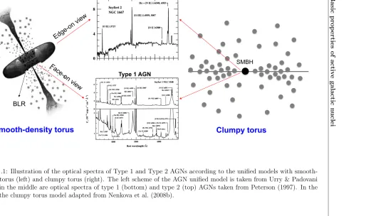
The general concept of the AGN unified model is that the central SMBH is surrounded by a parsec-scale accretion disk, in some cases, also accompanied by a powerful kiloparsec-scale jet. Further out from the accretion disk is the dusty torus on the kiloparsec-scale of few tens of parsecs (pc; where 1pc = 3.26 light years). Antonucci (1993) and Urry & Padovani (1995) provided a conceptual scheme for the model as shown in the left of Figure 1.1. Based on this scenario, different types of AGN can be identified according to their spectroscopic features caused by the orientation effect of viewing the smooth-density torus. Broad line regions (BLR) and narrow line regions (NLR) can both be observed from face-on view of torus, thus broad and narrow emission lines are presented in the spectra. Such AGNs are classified as “type 1”. However, with edge-on view, AGNs are classified as “type 2” that broad lines are obscured by torus and only narrow lines are presented in the spectra (see the middle spectra in Figure 1.1).

However, in the last few years, the model with smooth-density torus has been gradually substituted by a clumpy torus model which is a continuous cloud distribution from BLR toward the outer plane (Nenkova et al., 2002, 2008a,b). In this scenario, the spectroscopical classification remained but AGN types are defined by the probability for directly viewing the AGN rather than due to the orientation effect (Figure 1.1). Following, we describe the main continuum properties of type 1 and type 2 AGNs over the entire electromagnetic spectra, which are relevant to the need for computing photo-z in the later Chapter 2 and 3.

1.1.2 Properties of unobscured/type 1 AGNs spectra

(23)

1.1

Basic

prop

erties

of

activ

e

galactic

n

uclei

3

NLR

BLR

Smooth-density torus

Clumpy torus

SMBH

Type 2 AGN

Type 1 AGN

(24)

4 1. Introduction

Black hole

Corona

Jet

Accre0on disk

Clumpy torus

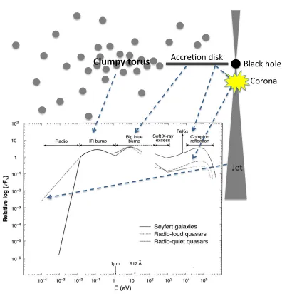
Figure 1.2: AGN spectral energy distribution from radio to X-ray. The subplot showing AGN continuum is adapted from Koratkar & Blaes (1999).

• X-ray

The X-ray emission includes two major components: (a) a primary power-law contin-uum; (b) and a reflection component. The intrinsic X-ray continuum is emitted from the

hot corona or jet, showing a power-law SED extending from∼1 keV to over 100 keV. The

power-law continuum can be fit by the form: Fν ∝ µ−Γ+1 ∝ ν−α, where Γ is called the

“photon index”, andαis referred to the “energy index”. For radio-loud AGNs, the spectra are generally flatter than radio-quiet AGNs because of the additional radiation emitted by inverse-Compton scattering of the electrons in the jet. For the “soft excess” between 0.2 keV and 1 keV, the physical origin is not yet clear. It could be an extension of the big blue bump or produced from warm gas located in the accretion disk or BLR.

(25)

1.1 Basic properties of active galactic nuclei 5

Compton scattering in the accretion disk or the cold clumpy gas around (e.g., clouds in

BLR or torus). This Compton reflection contains a continuum with a peak at ∼ 30 keV,

which is called “Compton hump” in the X-ray spectrum. In addition to the continuum, the Compton reflection also produces fluorescent emission lines (Reynolds, 1999). The iron Kα (Fe Kα) line at 6.4 keV is the most dominant feature in the X-ray spectrum that presents not only a narrow line from farther regions (e.g. torus or NLR), but also a broad

line component. Many works have found that the Fe Kα line shows a very broad and

asymmetric profile, which is supposed to be the consequence of relativistic Doppler shift and gravitational redshift (Tanaka et al., 1995; Nandra et al., 1997; Reynolds, 1997). This broad Fe Kαline profile is believed to be reflected from the innermost part of the accretion disk, and provides a powerful probe for understanding the conditions near SMBHs.

• Ultraviolet/optical

The UV and optical continuum of a type 1 AGN is attributed to the thermal emission from the accretion disk, and the spectrum can be approximately fit with a power law. The temperature of the accretion disk is in the range of 105₋₁₀6 _{K with a maximum energy}

flux at wavelength of ∼100˚A obtained by the Wien’s displacement law (eq. 1.1):

νmax =

2.8kT

h ≈3.6×10

16_Hz _(1.1)

This leads as a consequence to the “big blue bump” in the UV/optical continuum. The “soft X-ray excess” might be the high-energy end of this feature.

In addition to the “big blue bump”, broad emission lines are also one of the promi-nent characteristics in the UV/optical spectra of type 1 AGNs (see the spectrum in the bottom right of Figure 1.1). These lines are produced by photoionization in the BLRs of high-density clouds with gas density ≥109_cm−3_{. The width of the broad lines is generally}

in the range between∼500 km s−1 and∼10000 km s−1, with a typical value of 5000 km s−1 (Peterson, 1997). This broadened line profile is due to the Doppler shift caused by the bulk orbital motion in the BLR, and can be used as a probe for understanding the properties of the black holes (e.g., black hole mass; Krolik, 2001; Peterson et al., 2004).

• Infrared

The main characteristics of the IR continuum are : (a) a minimum at ∼1−2µm, and

(b) an “IR bump” at ∼ 10−30µm. The 1µm minimum corresponds to the sublimation

temperature of dust grains (usually between 1000 to 2000 K). The IR bump is due to the thermal emission of dust with a temperature between 50 and 1000 K. The origin the IR emission is still controversial. The continuum could be emitted by hot dust (<2000K) in the nuclear regions, or by the mechanism of reprocessing of the AGN primary emission, such as big blue bump.

• Submillimeter/radio

(26)

6 1. Introduction

have big differences between radio-loud and radio-quiet AGNs. For radio-loud objects, a continuum extends from the radio to the far-IR with a flatter spectrum shape. However, in a radio-quiet object, the spectrum decreases sharply from the far-IR, through the sub-millimeter to longer wavelengths (Fν ∝ να, α > 3). This feature is so-called “the sub

millimeter break”.

1.1.3 Properties of obscured/type 2 AGNs spectra

In practice, a large fraction of AGNs are obscured in the Universe and appear faint in optical. For these optically low-luminosity AGNs, the utilization of X-ray, IR, and radio wavebands provide alternative ways to select AGNs. Mart´ınez-Sansigre et al. (2006) used IR and radio criteria to select high-redshift type 2 quasars at z ≥ 2. They claimed that

the type 2 to type 1 AGN ratio is ∼3 : 1. Fiore et al. (2009) combined deep X-ray data

from Chandrawith IR data from Spitzer/MIPS to select heavily obscured Compton-thick

quasars. They found that the fraction of all types of AGNs to the total MIPS source

population is 49% ±10%. Buchner et al. (2015) also found that obscured AGNs with

NH>1022cm−2 account for 77% of the number density of the accreting SMBH population.

The AGN emission could be absorbed by dust or gas from the circumnuclear region or the host galaxy. Figure 1.3 gives a simple example scheme for the absorption from the torus and host. The level of absorption can be varied by the number, composition, and ge-ometry of the absorbers along the line of sight(e.g., Nenkova et al., 2008a,b; Elitzur, 2008; Buchner et al., 2015). Here we briefly describe the main features of the obscured/type 2 AGN spectrum.

• X-ray

For obscured AGNs, depending on the neutral hydrogen column density (NH), the

X-ray emission is absorbed via two mechanism: (1) photoelectric absorption and (2)

Compton scattering. With 1022 _< _N

H < 1.5× 1024cm−2 (Compton thin), the

obscu-ration is caused by photoelectric absorption which dominates below 3 keV. With NH >

1.5×1024cm−2(Compton thick), the absorption is dominant from 7 keV to 30 keV and is caused by Compton scattering. Figure 1.4 shows how the X-ray emission decreases with increasing values of NH, which represents the amount of gas along line of sight.

• UV/optical/IR

In type 2 AGN, the optical to UV continuum is absorbed by dust and the radiation is re-emitted at longer wavelengths. Therefore the spectrum is dominated by the stellar radiation from the host galaxy, and the big blue bump feature observable in type 1 AGN is not present in the type 2 AGN continuum. In addition, the optical spectrum only shows the narrow emission lines from the NLR, whereas the broad emission lines are absent because of the torus orientation effect that hides the BLR from the line of sight (see the spectrum in the upper right of Figure 1.1). The NLR has a relatively low density (i.e., ∼103_cm−3_),

(27)

1.1 Basic properties of active galactic nuclei 7

Figure 1.3: Schematic representation of the unobscured (type A) and obscured (type B, C, D) quasars. The inner black rings represent the torus surrounding the SMBH with a face-on (type A and C) or edge-on (type B and D) view. The shaded ellipses represent the dust in the host galaxy. The figure is from Mart´ınez-Sansigre et al. (2006) who claimed that the type 2 to type 1 AGN ratio is ∼3 : 1.

(28)

8 1. Introduction

usually less than∼500 km s−1, with typical values of 300−400 km s−1 (Peterson, 1997). Since star-forming galaxies also emit narrow lines, we can use their line ratios (e.g.,

[OIII]λ5007/Hβ) to distinguish type 2 AGNs from star-forming galaxies. However for

sources without spectroscopic data, it is difficult to tell the difference between type 2 AGNs and star-forming galaxies only by the UV/optical continua.

For the IR continuum, in addition to the dust radiation from the torus and the host, the spectrum also contains a large contribution from the reprocessing of optical to UV continuum. Therefore, in comparison with type 1 AGN continua, type 2 AGN continua show more flux in the IR waveband (Haas et al., 2003).

• Sub-mm/Radio

Because Sub-mm/Radio emission is not absorbed by dust or gas, the spectrum of type 1 and type 2 AGNs are similar in sub-mm/radio. Thanks to this characteristic, we can search for the heavily obscured AGNs that are missing in optical and soft X-ray wavebands using sub-mm/radio observations, as Mart´ınez-Sansigre et al. (2006) have demonstrated.

1.2 AGN evolution

The growth history of SMBHs can be reconstructed from the observations at low and high redshift. In this section, we first present the works from the multi-wavebands observa-tions at lower redshifts for constraining the SMBH growth in the local universe. Then we present the recent results at higher redshifts that have implications for the AGN and galaxy (co)evolution in the early Universe.

1.2.1 BH growth in the local Universe

In the local Universe, it has been well established that most galaxies harbor a SMBH in the center (Kormendy & Richstone, 1995; Magorrian et al., 1998). Since SMBHs mainly grow through matter accretion during the AGN phase (e.g., Soltan, 1982; Rees, 1984; Marconi et al., 2004), the fraction of galaxies with a SMBH in an active phase provides a measurement of the time scale of BH growth (i.e., AGN duty cycle). For example, Goulding et al. (2010) measured the AGN duty cycle for the IR-bright galaxies (LIR >

3× 109L) with low X-ray luminosities (average LX < 1043L). They found that the fraction of these galaxies is∼10−30% over theMBHrange∼106−108M. In Figure 1.5, Alexander & Hickox (2012) compared the result of Goulding et al. (2010) with Best et al. (2005) who showed a lower faction (∼ 5% over the MBH ∼ 106.5 −108M) of galaxies hosting optically luminous AGNs (defined as L[OIII] > 3×107ergs−1). In contrast to the

approximately constant fraction of IR-bright and optical-bright sources (crosses and filled squares in Figure 1.5, respectively), the fraction of galaxies with luminous radio AGN (L1.4 GHz > 1024W Hz−1) shows a strong dependence on the black hole mass, increasing

(29)

1.2 AGN evolution 9

Figure 1.5: AGN fraction as a function of BH mass for different AGN selections atz <0.3. Crosses: IR-bright sample from Goulding et al. (2010); filled squares: optical-bright sample from Best et al. (2005); open circles: radio luminous AGNs from Best et al. (2005). Figure taken from Alexander & Hickox (2012).

The AGN fraction is not only related to the BH mass, but also to the host stellar mass (M∗). For example, Xue et al. (2010) showed that the fraction of galaxies hosting luminous AGN (LX >1043L) atz ∼1 increases from ∼0.3% to 3% with M∗ increasing from∼1010_M

to∼1011M (Figure 1.6).

However, the rate of BH growth cannot just be measured using the AGN fraction. The mass accretion rate ( ˙MBH∝LEdd, where is the radiative efficiency) and Eddington ratio

(defined as λEdd =Lbol/LEdd) are required to measure the growth rate of SMBHs. For a

black hole growing for a given and an Eddington ratio λEdd, the growth time from an

initial mass Min to a final mass Mf in is derived by (Volonteri, 2010):

tgrowth = 0.45 Gyr

1−λEddln

Mfin

Min

(1.2)

In the local Universe, the typical accretion time scales of the AGN phase is∼107−109 yr (e.g., Marconi et al., 2004), and the majority of AGNs have Eddington ratio of λEdd ∼

10−6 ₋₁₀−3 _{(e.g., Goulding et al., 2010). With an Eddington ratio of} _λ

Edd ∼ 10−3, the

(30)

10 1. Introduction

Figure 1.6: AGN fraction as a function of stellar mass in redshift bins. The orange shaded region indicates the 1 σ confidence range of the sources with 41.9 < logL(0.5−8 keV) <

43.7 erg s−1_{, and purple points with uncertainties indicate the 1} _σ _{confidence range of the}

sources with 43.0<logL(0.5−8 keV) <43.7 erg s−1. Figure taken from Xue et al. (2010).

1.2.2 AGN evolution and BH growth in the distant Universe

The extensive data on SMBHs in nearby galaxies have provided a dramatic insight into the growth of BHs in the local Universe. However, to have an overall view of the history of BH accretion, we need to understand how BHs evolve with time, and how they grew in the early Universe. Studies of the luminosity function of optical quasars (bright AGNs with Lbol >1045erg s−1) in 1960-80s first discovered the existence of AGN evolution (e.g.,

Schmidt, 1968; Schmidt & Green, 1983; Boyle et al., 1988). The density and luminosity evolution atz >2 was not clear until the 1990s, when large spectroscopic surveys of high-z quasars were carried out. Surveys like the Two Degree Field (2dF) redshift survey and Sloan Digital Sky Survey (SDSS) have derived the optical luminosity function up toz ∼6, although the sample size becomes small at higher redshift (Boyle et al., 2000; Fan et al., 2001, 2006; Richards et al., 2006). Figure 1.7 presents the overall evolution of luminous

quasars using these two surveys. The space density of bright quasars peaks at z ∼ 2−3

and exponentially declines toward lower and higher redshift. It is still uncertain whether this trend continues at z > 6. To achieve higher redshifts, deeper and higher-resolution data in NIR waveband, e.g., KMOS and MOSFIRE, are needed to constrain the results.

Nevertheless, optical AGN selection is only effective for bright and unobscured AGNs, and provides marginal constraints on obscured or low-luminosity AGNs. X-ray surveys are more efficient for selecting AGNs and provide more complete census of the AGN population, including both unobscured AGNs and obscured AGNs (note that some of the heavily

obscured AGNs with NH are still missing in X-ray observations). For instance, X-ray

observations usingChandraand XMM-Newtonhave provided substantial number of X-ray

surveys in both deep or wide fields, e.g., Chandra Deep Fields (CDF) (Alexander et al.,

(31)

1.2 AGN evolution 11

Figure 1.7: The space density of luminous quasars as a function of redshift. The solid line is the best-fit model from the 2dF at z <2.5 (Boyle et al., 2000). The dashed line is the best-fitting model from the SDSS at 3.6 < z < 5 (Fan et al., 2001). The blue open circles represent the result from Richards et al. (2006), and the red solid circles represent the result at z ∼6 from Fan et al. (2006). Figure taken from D’Onofrio et al. (2012).

Cappelluti et al., 2009). These surveys provide more complete demographics of the AGN population.

In the X-ray luminosity function, lower X-ray-luminosity AGNs are found to peak at smaller redshift (as shown in Figure 1.8; Hasinger et al., 2005). This trend has been called “cosmic downsizing” which implies that more massive BHs underwent accretion processes in the distant Universe, whereas less massive BH did that in the nearby Universe (e.g., Cowie et al., 2003; Heckman et al., 2004). However the picture is still incomplete because we are missing a fraction of obscured AGNs. Recently many works have estimated such fraction, and found that it increases with redshift (e.g., Ueda et al., 2003; Hasinger, 2008; Aird et al., 2012; Buchner et al., 2015). This result implies that distant AGNs are surrounded by larger amounts of gas than AGNs in the local Universe. This raises questions: Where did the gas come from? Is there also at high redshift a connection between the amount of gas (and star formation rate) and BH accretion?

(32)

12 1. Introduction

Figure 1.8: The number density of type 1 AGNs as a function of redshift in X-ray luminosity bins. Figure adapted from Hasinger et al. (2005).

(33)

1.2 AGN evolution 13

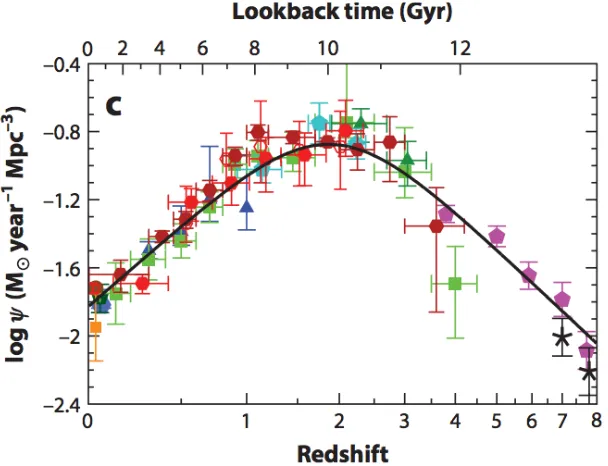
Figure 1.9: The cosmic star formation history. Figure taken from Madau & Dickinson (2014).

(34)

14 1. Introduction

1.3 Co-evolution of AGN and their hosts

The evolution of galaxy colors (and thus AGN host colors) can also be used for interpreting both galaxy evolution and how AGNs and galaxies influence each other. The studies are usually done by plotting the rest-frame color-magnitude diagram (CMD), originally using

U−V andMV. In this plot, late-type galaxies with bluer colors due to dusty star-forming

region and younger stellar population are well separated from early-type galaxies that have redder colors and older stellar population (e.g., Tully et al., 1998). Bell et al. (2004) first used the color-magnitude diagram showing this separation and introducing the concept of ”blue cloud” and ”red sequence” (Figure 1.11). They also used the diagram to study the galaxy evolution by investigating how the color distributions of early-type and late-type galaxies (i.e. passive or star forming galaxies) change with redshift. They revealed that the peak of the blue star-forming galaxies becomes redder toward the present day,

and the number density of these blue galaxies drops sharply since z ∼ 1. However, the

interpretation of galaxy colors can be misled by dust reddening. Brammer et al. (2009) indicated that the galaxy colors in the green valley (i.e., intermediate region between blue cloud and red sequence) are largely affected by dust extinction. They have showed that correcting for dust reddening makes the separation between red and blue galaxies much more clear.

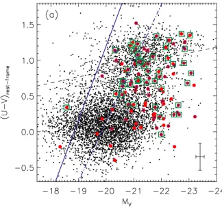
The CMD applied to AGN hosts can provide a direct comparison with normal galaxies distribution and evolution with the cosmic time. Several works have been done it atz ∼1 in small survey areas, e.g., the EGS and CDFS, where bright AGNs are few and the majority of sources are moderate-luminosity AGNs. In these fields, the X-ray luminosity of the AGNs have a weak correlation with their optical emission, and thus have host-dominated SEDs(e.g., Nandra et al., 2007; Silverman et al., 2008a; Xue et al., 2010). These works, purely based on spectroscopic samples limited to specific redshift ranges, found no apparent bimodality that instead is clearly presented for inactive galaxies (Figure 1.12). In addition, these studies also found a large fraction of X-ray selected AGNs placed in the green valley, which is considered as an evolutionary transition from blue cloud (star-forming galaxies) to red sequence (passive galaxies). This result suggests that AGN feedback may contribute to AGN evolution during the phase of green valley where host star formation are suppressed by powerful AGN. However, Cardamone et al. (2010a) claimed that the majority of green-valley AGN hosts are intrinsically blue but reddened by dust. They found a clean separation between red and blue galaxies after applying dust de-reddening.

(35)

1.3 Co-evolution of AGN and their hosts 15

Figure 1.11: The rest-frame color-magnitude diagram (CMD) for the R-selected galaxies

in the COMBO-17 at redshift range 0.2 < z < 1.1. The solid line is the linear fit of the red sequence, and the dashed line is the cut between red and blue galaxies. The color distribution at each redshift range is inset In the left bottom of each plot. Figure taken from Bell et al. (2004).

(36)

16 1. Introduction

Figure 1.12: Rest-frame color-magnitude diagram of AGN host galaxy colors in the ECDFS within the redshift range 0.4 ≤ z ≤ 1.1. Galaxies are shown in black dots while X-ray detected AGNs are displayed in red filled circles. Bulge-dominated AGN host galaxies are marked with blue filled circles. Open green squares indicate the AGNs with X-ray hardness ratios larger than 0.2. Figure taken from Silverman et al. (2008a).

1.4 Techniques for selecting high-z sources

(37)

1.4 Techniques for selecting high-z sources 17

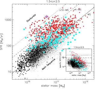
Figure 1.13: Stellar mass-star formation rate relation at 1.5 < z < 2.5. Red filled cir-cles and cyan squares represent the sources from the PACS-COSMOS and BzK-GOODS, respectively. The black dots indicate the BzK-COSMOS sources. The solid black line in-dicates the main sequence (MS) for star-forming galaxies at z ∼2 defined by Daddi et al. (2007). Figure taken from Rodighiero et al. (2011).

1999, 2003). They all use the same principle, namely use specific bands to identify typical features in the SEDs (e.g. Balmer break, Lyman break) at the redshift of interest. For instance, EROs are selected at z≥1 by the NIR color (R−K)vega >5 or (I−K)vega>4.

This extremely red color could come from old stellar populations in early-type and S0 galaxies, or from dusty starburst galaxies. Moriondo et al. (2000) studied the morphology of EROs and found that∼50−80% are indeed elliptical galaxies and ∼15% are irregular

and/or interacting galaxies. DRGs are chosen at z ≥ 2 by very red NIR colors with

(J−K)vega >2.3. This method was first defined by Franx et al. (2003) using deep VLT/

ISAAC data. The SEDs of these galaxies is characterized by the Balmer break which is shifted to the J-band at z ∼ 2. As shown in Figure 1.14, the (J −K)vega color changes

sharply around z ∼ 2, and can be an effective criterion to select sources at z ≥ 2. The

(38)

18 1. Introduction

tested empirically using the spectroscopic data from the K20 survey (K <20) and justified by the simulations of active and passive synthetic stellar population. For sources atz ∼3, the LBG technique is traditionally adopted to identify the high-z sample by the Lyman

break feature. This method uses UnGR color criteria to characterizes the UV continuum

emitted from the star-forming galaxies. We summarize these well-known color techniques in Table 1.1.

Figure 1.14: Color as a function of redshift for galaxies. The solid lines indicate single-age stellar population with age of 0.25, 0.5, and 1 Gyr. The dotted and dashed lines represent the stellar population with ages and reddening of 1 Gyr, E(B −V) = 0.15 and 100 Myr,

E(B−V) = 0.5, respectively. Figure taken from Franx et al. (2003).

Table 1.1: Color selections of high-z sources

Method Criteria Redshift range Nature Reference

Extremely Red Objects (R−K)vega≥5 z≥1 Old elliptical galaxy or Elston et al. (1988)

(ERO) dusty star-forming galaxies

Distant Red Galaxy (J−K)vega>2.3 z≥2 Old elliptical galaxy or Franx et al. (2003)

(DRG) dusty star-forming galaxies

BzKselection BzK= 1.4< z <2.6 Star-forming:BzK >−0.2 Daddi et al. (2004) (z−K)AB−(B−z)AB Passive:BzK <−0.2 and (B−z)AB>2.5

Lyman Break Galaxy (G−R)AB<1.2 z∼3 Rest-frame UV is absorbed Steidel et al. (1996)

(LBG) (Un−G)AB>(G−R)AB+ 1.0 by IGM, or by OB star Steidel et al. (2003)

19< RAB<25.5 in star forming galaxies

(39)

1.5 The challenges that we are facing 19

X-ray luminosity function, LBG technique is used to select high-z AGNs in Nandra et al.

(2005) and Aird et al. (2008, 2010). Moreover, Rangel et al. (2013) used BzK technique

to investigate the properties of X-ray selected AGNs. They found that passively

evolv-ing BzK galaxies have higher fraction of AGNs than star-forming BzK galaxies, which

contradict the idea of the coevolution between BH growth and star formation at z ∼ 2.

In Brusa et al. (2005), they used ERO selection to study the X-ray obscured quasars and found that majority of EROs are powered by the accretion activity of SMBH.

Due to large uncertainties caused by faint photometries, it is necessary to carefully select high-z sample. Aird et al. (2008) and Aird et al. (2010) pointed out the importance of using redshift probability distribution function, i.e.,P(z), to select high-z sample. They

simulated the function of P(z) for high-z sample selected by LBG method, applying an

additional weighting factor, w. The measurement of w considers the probability that a

source is located within a certain redshift range, and reduces the weight outside the target redshift range of LBG (see the detailed description in Section 5.3). This technique can provide effective number at high redshift and make the luminosity function more realistic. In this thesis, we will use the P(z) directly from our SED-fitting results of photo-z

computation for galaxies and AGNs, and apply the value of w to discuss the efficiency

of P(z)-technique and color methods. In the following section, we will demonstrate the challenges we are facing in the processes of running the SED-fitting.

1.5 The challenges that we are facing

For correctly modeling galaxy evolution, the availability of accurate redshifts for both normal galaxies and AGN is fundamental. Although redshifts measured via spectroscopic observations are very reliable, it is a problem to obtain large number of faint or high-redshift sources. Long exposure times are required for the faint sources typically found in deep field observations, and the relatively low sky density of AGN means that it is difficult to obtain large samples. Furthermore, for high-redshift sources, spectroscopic observations have observational limits such as: (1) the redshift range available to optical spectrographs and (2) the presence of the telluric OH lines that make it difficult to assign correct redshifts in near-infrared spectrographic observation from the ground. This restricts the availability of spectroscopic redshifts (spec-z), in particular for deep pencil-beam surveys. About 65% of sources in the Cosmic Assembly Near-IR Deep Legacy Survey (CANDELS; Grogin et al.,

2011; Koekemoer et al., 2011) in the GOODS-S region are fainter than H = 25, beyond

any reasonable spectroscopic limit. Similarly, only about 60% of the X-ray sources in the 4 Ms Chandra Deep Field-South (4Ms-CDFS) survey have reliable spec-z (Xue et al., 2011). Therefore, a large number of accurate photometric redshift (photo-z) are needed, particularly at the faint and high-redshift ends of the source distribution.

For normal galaxies, previous work has achieved photo-z accuracy (defined as 1.48×

median(₁₊|∆z_z|

(40)

20 1. Introduction

Extended Chandra Deep Field-South (ECDFS), photo-z for many samples are available in the literature (e.g., Zheng et al. 2004; Grazian et al. 2006a; Wuyts et al. 2008; Cardamone et al. 2010b; Luo et al. 2010; Dahlen et al. 2013 ). Although the accuracy reported in each paper is similar, discrepancies emerge when comparing photo-z for objects without spectroscopic information, especially at high redshift and for faint sources. In the following sections we demonstrate the challenges we are facing in photo-z computation.

1.5.1 SED templates for AGNs

Photo-z accuracy depends on the number and resolution of wavelength bands available as already shown by Ben´ıtez et al. (2009). One of the fields with the greatest number of photometric bands is the Great Observatories Origins Deep Survey-South (GOODS-S; Giavalisco et al., 2004a), which has been observed recurrently as new facilities have become available. The GOODS-S region is at the moment in a unique niche as homogeneous and deep data (including the exquisite X-ray coverage withChandra) are available. In addition

to intermediate-band photometry fromSubaru (Cardamone et al., 2010b) (Figure 2.3) and

deep Spitzer/IRAC data (Damen et al., 2011; Ashby et al., 2013), HST/WFC3 NIR data

from the CANDELS survey and J and KS bands from the Taiwan ECDFS Near-Infrared

Survey (TENIS; Hsieh et al., 2012) are now available. Deep NIR observations are necessary to obtain reliable redshifts at z > 1.5, where the prominent ∼4000˚A break shifts to NIR wavelengths. The availability of these new data will improve the accuracy of photo-z and push the good quality of photo-z to higher redshift.

The past decade has witnessed important developments in normal galaxy photo-z both by SED fitting and by machine learning techniques, and some of these improvements can be directly used for AGNs. For example, improvement of template-fitting photo-z by adding emission lines to the templates has been demonstrated by Gabasch et al. (2004, 2006) and Ilbert et al. (2006). Intermediate- and narrow-band (IB, NB) photometry is valuable to pinpoint emission lines in the SEDs (Ilbert et al., 2009; Salvato et al., 2009; Cardamone et al., 2010b; Matute et al., 2012), as simulations (e.g., Ben´ıtez et al., 2009) have predicted. However, even with the best data, photometric redshifts for AGNs remain challenging (Salvato et al., 2009, 2011). Photo-z errors for AGNs can have a significant impact on galaxy/AGN coevolution studies. For example, Rosario et al. (2013) found that at high redshifts the AGNs tend to have bluer colors than inactive galaxies, implying younger stellar populations and higher specific star formation rates in the AGN hosts. This result, as Rosario et al. mentioned, may be biased by the spectroscopic selection effect and photo-z errors leading to a bluer host color. The photo-photo-z failures are caused by observational limitations and improper templates used for photo-z computation. For example, Salvato et al. (2009, 2011) point out that due to the uncertainty of AGN/host galaxy contribution, we need to create proper AGN/galaxy hybrid templates to better model the AGN SEDs.

(41)

1.5 The challenges that we are facing 21

be caused e.g. by observational limitations, orientation effect, and different types of AGNs in different evolutionary phases. In addition, templates for AGNs are often empirically obtained from nearby AGNs where the slit size allows sampling of only the nuclear region of galaxies. At high redshift, the size of entire galaxies are comparable to the size of slits, so that both AGN and host emissions are included in slits or fibers. Therefore, the empirical low-redshift templates do not represent the SEDs of high-redshift AGNs, and hybrids that include both AGN and host contributions are necessary.

Secondly, we assumed that the SEDs are vary according to the viewing angle along line of sight. For instance, Seyfert 1 AGNs show relatively higher emission in the bluer part of the continuum than Seyfert 2s which have more of a galaxy-like continuum (see Figure 1.1). Thirdly, the varying contribution from AGN and host could be the result of different physical properties in different evolutionary phases. Figure 1.15 (Haas et al., 2003) gives one idea of how the shapes of the AGN continuum (assumed face-on view) evolve with the scale of dust distribution. With larger-scale dust obscuration, the stellar light from host galaxies highly affects the spectral slopes from UV to optical, which appears red and galaxy-like. In the more “clear” quasar stage, the strong characteristic UV excess appears and the SED becomes AGN-dominated. The reasons above explain how complicated the AGN SED is and why we need to build representative AGN-Galaxy hybrids.

In addition, as shown in Figure 1.1, emission lines are prominent features in AGN spectra, arising either from gas ionized by the central nuclei and/or star-forming regions. As shown above, the available intermediate-band data help characterize line features, so including emission lines in our templates makes our hybrids even more powerful when computing photo-z.

1.5.2 Multi-wavelength associations

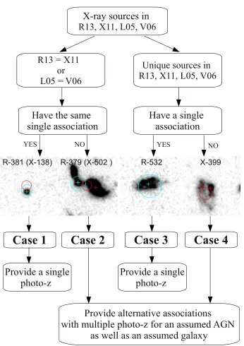
The situation for AGNs is further complicated by the need for an association with multi-wavelength data before a photo-z can be calculated. This makes the accuracy of positions for the X-ray sources and the method and data used for the associations of crucial impor-tance. In this thesis the impacts of both issues are studied as they could result in different counterparts (and often multiple potential counterparts can not be excluded). This is demonstrated in Chapter 2, where we compare the X-ray detections from Xue et al. (2011) and Rangel et al. (2013) in CDFS, and Lehmer et al. (2005a) and Virani et al. (2006) in ECDFS. In both pair of works, the X-ray data were the same but the way in which the data were analyzed gave different detections. A challenge for this thesis was to assess when the sources identified from different methods were the same and when not.

The offset in X-ray coordinates, even marginal, can give an different association to the multi-wavelength database, especially in crowded areas. A simple match in coordinates between X-ray and other data is not feasible, particularly for X-ray surveys with a lower

resolution than Chandra offered. But even at the resolution of Chandra, when NIR data

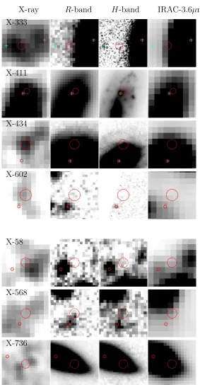
are deep and resolved like the HST/WFC3 data in CANDELS, multiple associations are possible (see Section 2.2).

(42)

Saun-22 1. Introduction

(43)

1.6 The outline of this work 23

ders 1992; Brusa et al. 2007; Laird et al. 2009; Luo et al. 2010; Xue et al. 2011; Civano et al. 2012), which relies on homogeneous coverage in a given visible or infrared band. Most works repeat the association for several different reference bands and finally choose a counterpart by comparing the results. The likelihood approach is based on the distance of a source from the X-ray detection and the probability of correct association is purely based on the comparison between the magnitude distribution of the sources in the field and the sources closest to the X-ray detection. Even when the likelihood approach is used on several different reference bands, the association is then done independently, selecting as counterpart the most frequent. Especially for X-ray surveys with large positional uncer-tainties, this can affect the result. We adopted instead a new bayesian code (Salvato et al. 2015, in prep.) developed in the high energy group at MPE which by use of priors, trying to compute the correct association by working simultaneously on more than two catalogs.

1.6 The outline of this work

This thesis is organized as follows:

• Chapter 1 reviews the basic properties and mechanisms defining an AGN at various

wavelengths. It also reviews our knowledge of AGN/galaxy (co)evolution in the local Universe and hints at the problems still open at high redshift. Finally, we introduces the difficulties that we will try to solve in this thesis.

• Chapter 2 introduces the fields and the multi-wavelength datasets we used in this

work. We demonstrate how we combined various photometries from different surveys and how we defined the most likely optical and near-infrared counterparts to the X-ray sources.

• In Chapter 3, we present the photo-z results for normal galaxies and for AGNs. In

particular we described the method of building a proper AGN-galaxy hybrid tem-plates for SED-fitting in detail. Moreover we demonstrate how the photo-z accuracy improves dramatically when considering templates with emission lines and how the presence of Intermediate bands improves on the overall results.

• In Chapter 4, we investigate the rest-frame color magnitude diagram as a function of redshift for both galaxies and AGN hosts. We made correction for dust extinction and AGN contribution, discussing which factor affects the host color distribution more, and compare the results with previous works. Unlike those which where limited

to z ∼ 1, thanks to the accuracy of our photo-z and to the care we took in the

AGN/galaxy decomposition, we can extend the analysis up to z ∼3.

• In Chapter 5, we firstly study the traditional color methods like the Lyman break

galaxy and BzK color-color selection. Then we test the robustness of our P(z)

(44)

24 1. Introduction

at z >3 with P(z) information, comparing with high-z AGN sample available from Fiore et al. (2012) who defined high-z sources in the same area but with a different technique.

• In Chapter 6 we summarize the main results of the thesis, presenting an outlook of

the next steps.

(45)

Chapter 2 The fields: CANDELS/GOODS-S,

CDFS, and ECDFS

The Chandra Deep Field South (CDFS) is an area of the sky with very low extinction by Galactic gas and dust. There are no bright stars (MV ≤ 14) within 300and the neutral

hydrogen column density is very low (NH∼8×1019cm−2; Giacconi et al., 2002). This allows

us to maximize the depth of X-ray observation, providing an opportunity to investigate the distribution and properties of supermassive black holes over cosmic time.

It is widely accepted that all AGNs in a field can not be identified using a single photometric band, which yields incomplete and partially overlapping subsample of the overall AGN population. A complete census of AGNs can only be achieved by combining the results from multi-wavelength selections. Nevertheless, a selection using X-ray band appears to be very efficient and rather complete for most classes of AGNs (Brandt & Hasinger, 2005). Therefore, in this work we identified AGNs using the X-ray detected

sources from theChandra space telescope.

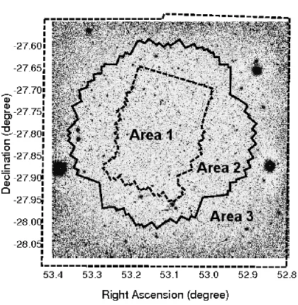
Taking advantage of this field for extragalactic observations, the CDFS area has been observed repeatedly with a large variety of facilities and instruments. As a result, numerous datasets with different bands and depths are available depending on the exact location. In this work, we collected the multi-wavelength data from the X-ray to Infrared in the GOODS-S, CDFS and Extended-CDFS (ECDFS) fields. Reliable X-ray-to-optical associ-ations and photometric redshifts can be obtained only when the data are homogeneous, and for this reason we split the area into subregions where the data are uniform. Three main regions share the same sets of data: Area 1 (∼176 arcmin2_{) is the region covered by}

CANDELS and GOODS-S, Area 2 (∼ 290 arcmin2) is the outer CDFS region

surround-ing CANDELS/GOODS-S, and Area 3 (∼ 435 arcmin2_{) is the ECDFS region outside the}

(46)

26 2. The fields: CANDELS/GOODS-S, CDFS, and ECDFS

Figure 2.1: Major areas defined in ECDFS. Background is the negativeJ+Ks image from

(47)

2.1 Data set 27

2.1 Data set

2.1.1 X-ray data

The X-ray catalogs to cross-match were obtained from the Chandra survey of 4Ms-CDFS

observations covering Area 1+2 and from the 250ks-ECDFS observations covering Area 3. Two independent groups (Xue et al., 2011; Rangel et al., 2013) have provided source catalogs for 4Ms-CDFS using different methods for data reduction and source detection. Similarly for Area 3, both Lehmer et al. (2005a) and Virani et al. (2006) have released X-ray source catalogs for the 250ks-ECDFS survey. We have cross-matched X-ray sources from both catalogs in each area.

For Areas 1+2 we used:

a. The 4Ms-CDFS source catalog of Xue et al. (2011) (hereafter X11) with 740 point-like X-ray sources. The sensitivity limits of the X-ray data are 3.2×10−17_{, 9}_.₁_×₁₀−18_,

and 5.5×10−17 erg cm−2 s−1 for the full (0.5–8 keV), soft (0.5–2 keV), and hard (2–8 keV) bands, respectively.

b. The 4Ms-CDFS source catalog of Rangel et al. (2013) (hereafter R13)1 _produced

using the analysis methodology of Laird et al. (2009). The catalog contains 569

point-like X-ray sources and has sensitivity limits 4.2 × 10−17, 1.2 × 10−17, and 8.8×10−17 _{erg cm}−2 _s−1 _{in the full, soft, and hard bands, respectively.}

For Area 3 we used:

c. The 250ks-ECDFS X-ray catalog from Lehmer et al. (2005a) (hereafter L05) with 762 sources in the entire ECDFS of which 457 are in Area 3 (i.e., outside the 4Ms-CDFS area). Catalog sensitivity limits are 1.1×10−16 erg cm−2 s−1 in the soft (0.5–2 keV) band and 6.7×10−16 _{in the hard (2–8 keV) band.}

d. The 250ks-ECDFS X-ray catalog from Virani et al. (2006) (hereafter V06) with 651 sources in the entire ECDFS of which 404 are in Area 3. Sensitivity limits are 1.7×10−16 and 3.9×10−16 erg cm−2 s−1 in the soft and hard bands, respectively.

2.1.2 Photometric data from UV to MIR

Altogether the CDFS region has been covered in up to 50 bands from ultraviolet (UV) to mid-infrared (MIR) as listed in Table 2.1 and Table 2.2. Table 2.3 summarizes the catalogs used in each area.

1. Area 1: In this region, we primarily used the CANDELS-TFIT multi-wavelength catalog of Guo et al. (2013, hereafter G13), which covers the CANDELS GOODS-S area with 18 broad-band filters (Figure 2.2) mostly from space observatories. The photome-try was based on template-fitting (TFIT; Laidler et al., 2007), using the high resolution

WFC3/H-band image to detect sources and define apertures, which were then used for

1 _{The 4Ms-CDFS X-ray catalog of R13 is available under [Surveys]} _> _{[CDFS] through the portal}

(48)

28 2. The fields: CANDELS/GOODS-S, CDFS, and ECDFS

2000 4000 6000 8000 10000

Wavelength (Angstrom) 0.0

0.2 0.4 0.6 0.8 1.0 1.2

Normalized transmission

FUV NUV U B V i z Y

2•104 4•104 6•104 8•104 1•105

0.2 0.4 0.6 0.8 1.0 1.2

YJH K IRAC1 IRAC2 IRAC3 IRAC4

Figure 2.2: Optical (top) and NIR/MIR (bottom) broad-band filter transmission curves.

4000 5000 6000 7000 8000

0.2 0.4 0.6 0.8 1.0

(49)

2.1 Data set 29

Table 2.1: Photometric Data in TFITCANDELS+IB catalog

Filter λeff FWHM 5σLimiting Depth Instrument Area

(˚A) (˚A) (AB mag) Telescope

FUVe 1543 228 25.69 GALEX 1

NUVe 2278 796 25.99 GALEX 1

U-CTIOa 3734 387 26.63 Blanco/Mosaic-II 1

U-VIMOSa 3722 297 27.97 VLT/VIMOS 1

F435Wa 4317 920 28.95/30.55f HST/ACS 1

F606Wa 5918 2324 29.35/31.05f HST/ACS 1

F775Wa 7693 1511 28.55/30.85f HST/ACS 1

F814Wa 8047 1826 28.84 HST/ACS 1

F850LPa 9055 1236 28.55/30.25f HST/ACS 1

F098Ma 9851 1696 28.77 HST/WFC3 1

F105Wa 10550 2916 27.45/28.45/29.45g HST/WFC3 1 F125Wa 12486 3005 27.66/28.34/29.78g HST/WFC3 1 F140Wa 13635 3947 26.89/29.84h HST/WFC3 1 F160Wa 15370 2874 27.36/28.16/29.74g HST/WFC3 1

Ks-ISAACa ₂₁₆₀₅ ₂₇₄₆ _25.09 _VLT/ISAAC ₁

Ks-HAWKIa ₂₁₄₆₃ ₃₂₅₀ _26.45 _VLT/HAWK-I ₁

3.6µm-SEDSa ₃₅₅₀₈ ₇₄₃₂ _26.52 _Spitzer/IRAC ₁

4.5µm-SEDSa ₄₄₉₆₀ ₁₀₀₉₇ _26.25 _Spitzer/IRAC ₁

5.8µm-GOODSa ₅₇₂₄₅ ₁₃₉₁₂ _23.75 _Spitzer/IRAC ₁

8.0µm-GOODSa ₇₈₈₄₀ ₂₈₃₁₂ _23.72 _Spitzer/IRAC ₁

IA427d ₄₂₅₃ ₂₁₀ _25.01 _Subaru ₁

IA445d ₄₄₄₅ ₂₀₄ _25.18 _Subaru ₁

IA464d ₄₆₃₁ ₂₁₆ _24.38 _Subaru ₁

IA484d ₄₈₄₃ ₂₃₀ _26.22 _Subaru ₁

IA505d ₅₀₅₉ ₂₃₄ _25.29 _Subaru ₁

IA527d 5256 243 26.18 Subaru 1

IA550d 5492 276 25.45 Subaru 1

IA574d 5760 276 25.16 Subaru 1

IA598d 6003 297 26.05 Subaru 1

IA624d 6227 300 25.91 Subaru 1

IA651d ₆₄₉₁ ₃₂₄ _26.14 _Subaru ₁

IA679d ₆₇₇₈ ₃₃₉ _26.02 _Subaru ₁

IA709d ₇₀₇₀ ₃₂₁ _24.52 _Subaru ₁

IA738d ₇₃₅₆ ₃₂₄ _25.93 _Subaru ₁

IA768d ₇₆₇₆ ₃₆₆ _24.92 _Subaru ₁

IA797d ₇₉₆₂ ₃₅₄ _24.69 _Subaru ₁

IA827d ₈₂₄₃ ₃₃₉ _23.60 _Subaru ₁

IA856d ₈₅₆₂ ₃₂₄ _24.41 _Subaru ₁

a_{CANDELS-TFIT catalog (Guo et al., 2013)}

d_{IB-TFIT catalog (J. L. Donley et al. 2015, in preparation)} e_{GALEX DR6/7}

f _{Measurements from two regions: GOODS-S and HUDF09. See the detail in Guo}

et al. (2013)

g_{Measurements from three regions: CANDELS wide, deep, and HUDF09. See Guo}

et al. (2013) for details.

h_{Measurements from two regions: 3D-HST and HUDF12. This is an updated version}

Hsu, Li-Ting (2015): Photometric redshifts of faint X-ray sources: paving the way towards the study of AGN/galaxy co-evolution over cosmic time. Dissertation, LMU München: Fakultät für Physik

Photometric redshifts of faint X-ray

sources: paving the way towards the

study of AGN/galaxy co-evolution over

cosmic time

Li-Ting Hsu

Photometric redshifts of faint X-ray

sources: paving the way towards the

study of AGN/galaxy co-evolution over

cosmic time

Li-Ting Hsu

Dissertation

an der Fakult¨

at f¨

ur Physik

der Ludwig–Maximilians–Universit¨

at

M¨

unchen

vorgelegt von

Li-Ting Hsu

aus Taoyung, Taiwan

Contents

List of Figures

List of Tables

Zusammenfassung

Abstract

Chapter 1

Introduction

1.1

Basic properties of active galactic nuclei

1.1.1

AGN unified model

1.1.2

Properties of unobscured/type 1 AGNs spectra

Smooth-density torus

Clumpy torus

Black hole

Corona

Jet

Accre0on disk

Clumpy torus

1.1.3

Properties of obscured/type 2 AGNs spectra

1.2

AGN evolution

1.2.1

BH growth in the local Universe

1.2.2

AGN evolution and BH growth in the distant Universe

1.3

Co-evolution of AGN and their hosts

1.4

Techniques for selecting high-z sources

1.5

The challenges that we are facing

1.5.1

SED templates for AGNs

1.5.2

Multi-wavelength associations

1.6

The outline of this work

Chapter 2

The fields: CANDELS/GOODS-S,

CDFS, and ECDFS

2.1

Data set

2.1.1

X-ray data

2.1.2

Photometric data from UV to MIR