University of Windsor University of Windsor
Scholarship at UWindsor
Scholarship at UWindsor
Electronic Theses and Dissertations Theses, Dissertations, and Major Papers 2010
An Efficient Design of 2-D Digital Filters Using Singular Value
An Efficient Design of 2-D Digital Filters Using Singular Value
Decomposition and Genetic Algorithm with Canonical Signed Digit
Decomposition and Genetic Algorithm with Canonical Signed Digit
(CSD) Coefficients
(CSD) Coefficients
Bashier Elkarami
University of Windsor
Follow this and additional works at: https://scholar.uwindsor.ca/etd
Recommended Citation Recommended Citation
Elkarami, Bashier, "An Efficient Design of 2-D Digital Filters Using Singular Value Decomposition and Genetic Algorithm with Canonical Signed Digit (CSD) Coefficients" (2010). Electronic Theses and Dissertations. 8123.
https://scholar.uwindsor.ca/etd/8123
An Efficient Design of 2-D Digital Filters Using Singular Value
Decomposition and Genetic Algorithm with Canonical Signed
Digit (CSD) Coefficients.
by
BASHIER ELKARAMI
A Thesis
Submitted to the Faculty of Graduate Studies through Electrical and Computer Engineering in Partial Fulfillment of the Requirements for the Degree of Master of Applied Science at the
University of Windsor
Windsor, Ontario, Canada 2010
1*1
Library and Archives CanadaPublished Heritage Branch
395 Wellington Street OttawaONK1A0N4 Canada
Bibliotheque et Archives Canada Direction du
Patrimoine de I'edition 395, rue Wellington OttawaONK1A0N4 Canada
Your file Votre reference ISBN: 978-0-494-80231-1 Our file Notre r6f6rence ISBN: 978-0-494-80231-1
NOTICE: AVIS:
The author has granted a
non-exclusive license allowing Library and Archives Canada to reproduce,
publish, archive, preserve, conserve, communicate to the public by
telecommunication or on the Internet, loan, distribute and sell theses
worldwide, for commercial or non-commercial purposes, in microform, paper, electronic and/or any other formats.
L'auteur a accorde une licence non exclusive permettant a la Bibliotheque et Archives Canada de reproduire, publier, archiver, sauvegarder, conserver, transmettre au public par telecommunication ou par I'lnternet, preter, distribuer et vendre des theses partout dans le monde, a des fins commerciales ou autres, sur support microforme, papier, electronique et/ou autres formats.
The author retains copyright ownership and moral rights in this thesis. Neither the thesis nor substantial extracts from it may be printed or otherwise reproduced without the author's permission.
L'auteur conserve la propriete du droit d'auteur et des droits moraux qui protege cette these. Ni la these ni des extraits substantiels de celle-ci ne doivent etre imprimes ou autrement
reproduits sans son autorisation.
In compliance with the Canadian Privacy Act some supporting forms may have been removed from this thesis.
Conformement a la loi canadienne sur la protection de la vie privee, quelques formulaires secondaires ont ete enleves de cette these.
While these forms may be included in the document page count, their removal does not represent any loss of content from the thesis.
Bien que ces formulaires aient inclus dans la pagination, il n'y aura aucun contenu manquant.
DECLARATION OF ORIGINALITY
I hereby certify that I am the sole author of this thesis and that no part of this thesis has been published or submitted for publication.
I certify that, to the best of my knowledge, my thesis does not infringe upon anyone's copyright nor violate any proprietary rights and that any ideas, techniques, quotations, or any other material from the work of other people included in my thesis, published or otherwise, are fully acknowledged in accordance with the standard referencing practices. Furthermore, to the extent that I have included copyrighted material that surpasses the bounds of fair dealing within the meaning of the Canada Copyright Act, I certify that I have obtained a written permission from the copyright owner(s) to include such material(s) in my thesis and have included copies of such copyright clearances to my appendix.
ABSTRACT
In this thesis, the design of 2-D filters by SVD is proposed. This technique reduces the complexity of the designed 2-D digital filters by decomposing it into a set of 1-D digital filters in zl and z2 connected in cascade.
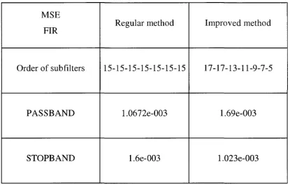
The design by SVD can be improved by varying the order of 1-D digital filters in each section based on their corresponding singular values. It is shown that by assigning higher order filters to the sections with greater singular values (SVs), and lower order filters to the sections with lower SVs, a sizable reduction in the total number of required multiplications is achieved.
A Genetic Algorithm (GA) is used to design each of the 1-D filters instead of classical optimization.
Canonical signed digit system is used to represent filters' coefficients. CSD helps to improve the efficiency of multiplications and thus increase the throughput rate.
DEDICATION
ACKNOWLEDGEMENTS
I would like to express my sincere appreciation to Dr. M. Ahmadi for
his guidness through out my thesis. His advices, patience, and encouragment
helped me to successfully complete my research.
I thank my wife, parent, and brothers for their support and help.
TABLE OF CONTENTS
DECLARATION OF ORIGINALITY iii
ABSTRACT iv DEDICATION v ACKNOWLEDGEMENTS vi
LIST OF TABLES x LIST OF FIGURES xiii CHAPTER
I. INTRODUCTION
1.1 Introduction 1 1.2 Characterization of 1-D FIR and IIR filters 2
1.2.11-D FIR filters 2 1.2.2 1-D IIR filters 3 1.3 Design Technique for 1-D FIR filters 4
1.4 Design Technique for 1-D IIR filters 4
1.5 Two Dimensional Digital Filters 5 1.6 Applications of 2-D digital filters 5
1.7 Characterization of 2-D FIR and IIR filters 6
1.7.1 2-D FIR filters 6 1.7.2 2-D IIR filters 7 1.7.3 Separable product 2-D IIR filters 8
1.7.4 Separable denominator non-separable numerator 2-D IIR
filters 8 1.7.5 Symmetry property of 2-D filters with separable
denominator non-separable numerator 9
1.8 Design techniques 10 1.8.1 2-D FIR digital filters 10
1.8.2 2-D IIR digital filters 11
1.10 Conversion from 2's - complement number to CSD numberl6
1.11 Organization of this thesis 22 II. SINGULAR VALUE DECOMPOSITION
2.1 Introduction to Singular Value Decomposition (SVD) 23
2.2 Example 25 III. GENETIC ALGORITHM
3.1 Introduction 31 3.2 GA Cycle 32 3.3 Population initialization 33
3.4 Fitness functions 33 3.5 Reproduction 34 3.6 Crossover 35 3.7 Mutation 37 3.8 Example 37 3.9 GA Analysis 49 3.9.1 The Effect of Reproduction 49
3.9.2 The Effect of Crossover Operation 50
3.9.3 The Effect of Mutation 50 IV. DESIGN 2-D DIGITAL FILTERS BY SVD
4.1 Design recursive digital filters 52
4.2 ERROR COMPENSATION 58 4.3 Design nonrecursive digital filters 62
4.4 Advantages of SVD 69 4.5 Improved design 70
4.6 Examples 71 4.7 Conclusion 96 V. DESIGN 2-D DIGITAL FILTERS BY GENETIC ALGORITHM
5.1 Design digital filters by genetic algorithm 97
5.2 Modification of GA 97 5.2.1 Initial population 97 Throughout this thesis, the population size is 80 nd the maximum
iterations is 100 98 5.2.2 Fitness function 98 5.2.3 Reproduction, Crossover and mutation operations 98
5.3 Examples 102 5.4 Design with CSD=5 126
5.4.1 low pass FIR 126 5.4.2 Band pass FIR 131 5.4.3 High pass FIR 136
VI. CONCLUSION 141
REFERENCES 142
LIST OF TABLES
Table 1.1 Shows how much reduction we can get of each class 10
Table 1.2 Illustrate the conversion's steps of 441 18 Table 1.3 Shows comparison between 2's-comlement and CSD
in non-zero digits 20 Table 4.1 Coefficients comparison between regular SVD and
improved SVD of 4th Order IIR 73
Table 4.2 Error comparison between improved and regular SVD
of 4th order IIR 74
Table 4.3 Coefficients comparison between improved and regular
SVD of 17th Order FIR 77
Table 4.4 Error comparison between improved and regular SVD
of 17th order FIR 78
Table 4.5 Coefficients comparison between improved and regular
SVD of 15th Order band pass FIR 84
Table 4.6 Error comparison between improved and regular SVD
of 15th order Band pass FIR 85
Table 4.7 Error comparison between improved and regular SVD
of 31st order high pass FIR 91
Table 4.8 Error comparison between improved and regular SVD
of 31st order high pass FIR 92
Table 5.1 The numerator and denominator coefficients of 1-D filter (f 1) of the first section of the 4th order IIR regular
filter (fl) of the first section of the 4th order IIR
improved method 106 Table 5.3 Error comparison between improved and regular SVD
of 4th order IIR with 4 CSD 107
Table 5.4 The coefficients of 1-D filter (fl) of the first section
of the 17th order FIR regular method 110
Table 5.5 The coefficients of 1-D filter (fl) of the first section
of the 17th order FIR improved method 112
Table 5.6 Error comparison between improved and regular SVD
of 17th order FIR with 4 CSD 113
Table 5.7 The coefficients of 1-D filter (fl) of the first section of
the 15th order band pass FIR regular method 116
Table 5.8 The coefficients of 1-D filter (fl) of the first section of
the 15th order band pass FIR improved method 118
Table 5.9 Error comparison between improved and regular SVD
of 15th order band pass FIR with 4 CSD 119
Table 5.10 The coefficients of 1-D filter (fl) of the first section of
the 31st order high pass FIR regular method 122
Table 5.11 The coefficients of 1-D filter (fl) of the first section of
the 31st order high pass FIR improved method 124
Table 5.12 Error comparison between improved and regular SVD
of 31st order high pass FIR with 4 CSD 125
Table 5.13 The coefficients of 1-D filter (fl) of the first section of
the 17th order low pass FIR regular method with 5 CSD 127
Table 5.15 Error comparison between improved and regular SVD
of 17th order FIR with 5 CSD 130
Table 5.16 The coefficients of 1-D filter (fl) of the first section of
the 15th order band pass FIR regular method with 5 CSD 132
Table 5.17 The coefficients of 1-D filter (fl) of the first section of the 15th order band pass FIR improved regular method
with 5 CSD 134 Table 5.18 Error comparison between improved and regular SVD
of 15th order band pass FIR with 5 CSD 135
Table 5.29 The coefficients of 1-D filter (f 1) of the first section of
the 31st order high pass FIR regular method with 5 CSD 137
Table 5.20 The coefficients of 1-D filter (fl) of the first section of
the 31st order high pass FIR improved method with 5 CSD 139
Table 5.21 Error comparison between improved and regular SVD
LIST OF FIGURES
Fig. 1.1 Flowchart can be used to convert 2's-complements then to CSD 19
Fig. 3.1 GA cycle 33 Fig. 3.2 The roulette wheel 35
Fig. 3.3 One-point Crossover 36 Fig. 3.4 Mutation operation 37 Fig. 3.5 Flow chart of GA 38 Fig. 4.1 Realization of quadrantally symmetric2-D filter 59
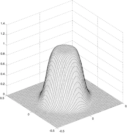
Fig. 4.2 The 4th order low pass IIR 60
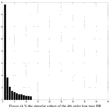
Fig. 4.3 The singular values of the 4th order low pass IIR 61
Fig. 4.4 The 17th order low pass FIR 67
Fig.4.5 The singular values of the 17th order low pass FIR 68
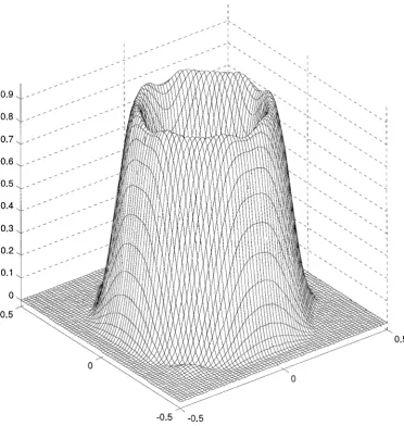
Fig.4.6 The 4th order low pass IIR by improved method 72
Fig.4.7 The 17th order low pass FIR by improved method 76
Fig.4.8 The singular values of the 15th order band pass FIR 80
Fig.4.9 The 15th order band pass FIR by regular method 81
Fig.4.10 The 15th order band pass FIR by improved method 83
Fig.4.11 The singular values of the 31st order high pass FIR 87
Fig.4.12 The 31s order high pass FIR by regular method 88 Fig.4.13 The 31s order high pass FIR by improved method 90
Fig.5.1 Flow chart of modified GA 101 Fig.5.2 The 4th order low pass IIR by regular method by GA and 4 CSD 102
Fig.5.3 The 4thorder low pass IIR by improved method by GA and 4CSD105
Fig.5.4 The 17thorder low pass FIR by regular method by GA with 4CSD109
Fig.5.7The 15th order bandpass FIR by improved method by GA & 4 CSD 177
Fig.5.8The 31storder high pass FIR by regular method by GA and 4CSD 121
Fig.5.9The 31storder high pass FIR by improved method by GA &4CSD 123
Fig.5.10 The 17th order low pass FIR by regular method with 5 CSD 126
Fig.5.1 IThe 17th order low pass FIR by improved method with 5 CSD 128
Fig.5.12The 15th order band pass FIR by regular method with 5 CSD 131
Fig.5.13 The 15th order band pass FIR by improved method with 5 CSD 132
Fig. 5.14 The 31st order high pass FIR by regular method with 5 CSD 136
CHAPTER I
INTRODUCTION
1.1 Introduction
Digital signal processing is one of the most powerful techniques concerned with transformation and manipulation of signals and their information. Signals are represented as sequence of numbers and they are processed by using digital means in accordance with specific computational algorithms that can be implemented on computers. Since the implementation cost of DSP has decreased significantly, the applications of DSP have vastly increased in many diverse fields. DSP can be found in mobile phones, multimedia computers, video recorders, CD players, hard disk driver controllers, and modems. Digital signal processing can deal with one dimensional signals or multidimensional signals represented as multidimensional arrays such as sampled images. The processing of 1-D DSP and 2-D DSP are conceptually similar where many operations performed on 1-D DSP are the same as those performed on 2-D DSP. Except that the amount of data involved in 2-D DSP are higher than these in 1-D DSP.
transmission [1, 2, 3, and 4]. To reduce the power consumption and implementation cost of digital filters, the complexity of multipliers has to be reduced. One way of doing that is by using CSD representation system to represent filter coefficients which reduces the number of partial products being summed [5, 6, and 7]. Generally, digital filters are divided into two basic types: Recursive digital filters known as Infinite impulse response IIR and Finite impulse response nonrecursive digital filters [8, 9, 10, 11, and 12].
1.2 Characterization of 1-D FIR and IIR filters
1.2.11-D FIR filters
In FIR digital filters, one whose impulse response is of finite duration, the current output, y (n ), is calculated from the current and previous input value as shown bellow;
N
yW^^^xin-i) (1.1)
The z-transfer function of FIR of order N is given as the following:
H(z) = jra
iZ-' (1.2)
i=0The magnitude and phase response of the filter at a particular frequency 0)
i ftsr
is given by replacing Z with e in the transfer function.
H(z) = f,a
le-
JC0lT(1.3)
i=01.2.2 1- D IIR filters
In IIR digital filters, whose impulse response continues forever, the current
output ,y(n), is calculated from the current and previous input values as well
as the previous output and therefore,
N M
y(n) = Y,b
lx(n-i)-Y
ja
Jx(n-j) (1.4)
i=0 j=0
If M = N the z-transfer function is:
N
»(?) = -£ = ^
7=0
B(Z) (1.5)
B(z)*0and \z\>l
The magnitude and phase of the filter at a particular frequency (O is given
by replacing Z with C in the transfer function.
N
-icaT
2>,
e-"
1=0 N
2>, *-"
H(z) = -^ (1.6)
,-JtOlT
1=0
1.3 Design Technique for 1-D FIR filters
One of the most common design methods for 1-D FIR is the Fourier series in conjunction with windows. The most common used windows are Hann, Hamming, and Kaiser [2, 12]. Linear and nonlinear programming is another method which includes optimization technique such as least square error.
1.4 Design Technique for 1-D IIR filters
The most traditional method is transforming from analog filters such as Butterworth, Chebysheve, elliptical, and Bessel filters, to digital filters [13]. The most commonly used transformation is the Bilinear transformation. Similar to 1-D FIR, optimization technique can be used to design IIR filters.
and vast amount of computations comparing to IIR to satisfy the same specifications.
1.5 Two Dimensional Digital Filters
2-D digital filters are computational algorithms that transform a 2-D input sequence of numbers into a 2-D output sequence according to pre-specified rules. Similar to 1-D digital filters, 2-D digital filters can be divided to two basic types: Finite impulse response (FIR) and Infinite impulse response (IIR). The objective of 2-D digital filters is usually being either enhancement of an image to make it more acceptable to human eye, or removal of the effect of some degradation mechanisms, or separation of features to facilitate identifications and measurement by human or machine.
1.6 Applications of 2-D digital filters
remove the noise comes with real data because of vehicle instability or in the water [22]. 2-D digital filters are used to remove interference in radio astronomy signals so they can obtain much clearer image of the stars and galaxies [23]. 2-D digital filters are used for efficient image encoding specially when digital transmissions and storage of image is needed and the amount of bits required is huge like in broadcast TV teleconference. 2-D digital filters are used in satellite images to getred of various image degradation occure because of random noise, interference geographical distortion.
1.7 Characterization of 2-D FIR and IIR filters
1.7.1 2-D FIR filters
Similar to 1-D FIR filters, 2-D FIR can be written as
N N
y(m,n) = ]T]TaO' J) x(m-i ,n-j) (1.7)
i=0j=O
The z-transfer function of 2-D FIR digital filters is as follows:
N N
i=0 j=0
N N
i=0 j=0
(1.9)
1.7.2 2-D IIR filters
Similar to 1-D IIR filters, 2-D IIR can be written as
N N N N
y(m,n) = Y^aiiJ )x(m-i,n-j) - XS^O' J)x(m~i,n-j)
i=0 j =0 i=0 j =0
(1.10)
The z-transfer function of 2-D IIR digital filters is as follows:
N N
H(
zz ) = '
= Q 7 = 0* = 0 ; = 0
B ( z „ z
2) * 0 f) z
t>1
(=1(1.11)
And the frequency response is:
f
jj^a(i,j)e-^
Te-^
TH(z z )=
l=Oj=0i=0 j=0
(1.12)
There are some subclass IIR filters that should be introduced as follows:
1.7.3 Separable product 2-D IIR filters
The filter of this sub-class is a cascade of 1-D filters [24, 25, 26, and 27].The advantages of this sub-class are reducing the problem from 2- D to 1-D, and reducing the stability problem to 1-D. However, the shape of the cutoff boundary has to be rectangular.
H(z
l,z
2) = H
l(z
l)H
2(z
2)
(1.13) N
H
k(z
k ^ k / N k) = ^
J=0
1.1 A Separable denominator non-separable numerator 2-D IIR filters This filter has the advantages of separable product filters but not their disadvantages. Circular symmetric, quadrantal, and octagonal symmetric magnitude response is achievable.
N N
H(z,,z
2) =
Y,J]a(iJ)z;
lz
2~
Ji=0 j=0
\i=0 )\]=0
1.7.5 Symmetry property of 2-D filters with separable denominator non-separable numerator.
Some filters have some desirable properties as follows:
i-Central Symmetry
In this sub-class, the magnitude response is equal in first and third quadrants and in second and fourth. [28, 29, 30, 31]
ii-Quadrantal Symmetric
In this sub-class, the magnitude response is equal in all four quadrants [28,32].
aU = am - l j ~a\m-j ~am-lm-j blj=h2j
iii-Octagonal Symmetric
Filter class General class
Central class Quadrantal
class Octagonal class
Multiplications 2 ( m + l )2
(m + l)(m + 3)
M 214 + 3m + 3 MA2/4+3m+3
( M2+ 2 2 m + 2 4 ) / 8
Reduction 0
M2- l
7 M2/ 4 + m - l
( 1 5 M2+ 1 0 m - 8 ) / 8
Table (1.1) shows how much reduction we can get of each class
1.8 Design techniques
1.8.1 2-D FIR digital filters
1.8.2 2-D IIR digital filters
Frequency - domain technique offers flexibility in design and implementation. The optimization technique depends on minimizing the error between the ideal filter and the designed filter [5]. The transformation technique is the simplest and fastest technique, though filters designed by it are not optimum. One of the most power transformations is double bilinear. Separable technique is simple and economical to implement because it reduces the design problem from 2-D to 1-D filters. Filters designed by this technique do not satisfy the specifications as closely as the non-separable filters.
1.9 Number Systems
In digital computer system, different number system may represent the same value of data in different form. Number systems can be classified into three types; weighted number system, unweighted number system, and the homomorphic number system. Weighted number system can be represented in fixed point or floating point based format. This type includes decimal, binary, octal, hexadecimal, one's complement, and two's complement. Unweighted number system is based on using different radix to scale a number like in residue number system. Homomorphic number system is rooted from the idea of abstract algebra. Fixed point and floating point of weighted number system are commonly used in designing digital filters and the following is the brief description of some of them.
1.9.1 Two's complement system
This system uses the left most bit to determine whether the number is positive or negative. For positive number, zero is assigned to the left most bits. For negative number, one is assigned to the left most bit. To convert to two's complement from decimal, first convert to binary then complement all bits then add one.
1.9.2 Signed Magnitude Number System
N-l
A=^
x 2'
_ 1 (1.15)i=0
1.9.3 Signed digit number system
In this system, each bit could take 1,-1, or 0
N-l
A=Y
db,x2-'
(1.16)(=0
1.9.4 Canonical Signed Digit Coefficients
The canonical signed-digit (CSD) number system is based on the signed digit number system which allows individual digits to have a sign as well as a value.
Digit =
r
2
, . , . , i, u, i , . , . ,
r
2
(1.17)The ternary number system where r=2 is used which allows the digits to have values of 1,0,1. Where 1 denotes -1.
0.01 = lx2~
2=0.25
and
O.Tl = - l x 2 - ' + l x 2 -
2= - 0 . 2 5
0.01 and 0.11 are two different representations with the same value.
However, for any given value of two or more redundant representations in signed digit system, there will be only one CSD representations. Two restrictions must be met in CSD system, first no two non-zero digit to be adjacent. Second, there is a limit on the number of non-zero digits that may be presented in a CSD number. A number in CSD number system is represented as a sum and difference of power of two as the following:
L
x=Y,S
kx2'
Pk(1.18)
k=l
Where
k =l:M
Pke{0,l,2,....,M -1} S k is ternary digits S k 1,0,1 M is a pre-specified word length. L is the number of non-zero digits
For example, the following three numbers are converted to CSD system with M=12 and L=3
0.8594 = 2° - 2"
3- 2~
6= 00001.00TOOlO
1.6875 = 2
1- 2
-2- 2'
4= 00010.0 ToTOOO
50 = 2
6- 2
- 2+ 2
1= 1010010.00000
63 = 2
6- 2° = 100000 T.00000
The example clearly shows that all the non-zero digits are separated by at least one zero digit.
The fewer non-zero digits give the CSD system an advantage over binary system where the fewer non-zero digits mean fewer products in multipliers. Multipliers in digital filters are performed with shifters, adders and subtractions. The multiplier repeatedly shifts one or more bit position and adds to a partial product according to the bit pattern of the multiplicand. While shift operations execute quickly, addition operations slower and comprise the bulk of multiplications time.
In binary system:
0 0 0 0 1 1 0 1 13 0 0 0 0 1 1 1 0 14
0 0 0 0 0 0 0 0
0 0 0 0 1 1 0 1 add 0 0 0 0 1 1 0 1 add 0 0 0 0 1 1 0 1 add
0 0 0 0 1 0 1 1 0 1 1 0 182
In CSD system:
0 0 0 1 0 T O 1 13 O O O l O O l O 14
0 0 0 0 0 0 0 0
0 0 0 l O l O I subtract 0 0 0 1 0 I 0 1 shift 2 t i m e s
0 0 0 0 1 0 1 1 0 1 1 0 182
This example shows that the binary system needs four additions but the CSD system needs one subtraction which is the same as additions, thus reducing the complexity of multipliers. Therefore CSD system reduces the cost of designing digital filters since multiplications consume most of the power and implementations cost.
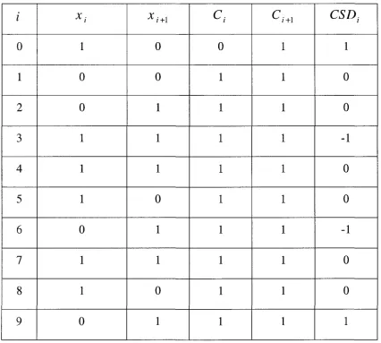
1.10 Conversion from 2's - complement number to CSD number
-i*. -••• -A/ -i ^\> o . . . . * \
We start from the least significant bit LSB (the rightmost) of x to the most significant bit MSB of x and we deal with two bits at the time.
1-let x; = x , ^ , C0 = 0
2~for i = 0 j - 1 , l e t C! + 1= x , x; + 1 + X iC( + xl + 1CI + 1
Where
C( + 1 is the carry of the step i+1
Ct is the carry of the step i The'+'is the logical OR
3-for i=0 j - 1 , let C S D , = x
(+ C , - 2 C
I + 1Fxample:
We convert 441 to 2's-complements then to CSD
441 = 01 101 1 1001 (2's ) = 100 l 0 0 TO 01 ( C S D )
Table 2 and flowchart 1 illustrate the conversion's steps
i
0
1
2
3
4
5
6
7
8
9
* /
1
0
0
1
1
1
0
1
1
0
X i+\
0
0
1
1
1
0
1
1
0
1
c
t0
c
i+l CSDi1
0
0
-1
0
0
-1
0
0
1
00.10
Ct=0 Carry=0
T
Start
i=l Carry=0 Xn=Xn-l
Ci=l Carrv=0
00
Ci=-I Carry=1
i *_
U
i=i+l
Yes
x, 01.11
v
To show the significant of CSD over 2's-complements, we compare between them by converting same number from decimal to 2's-complements then to CSD and calculate the non-zero digits in both of them.
DEC
7
13
14
15
63
-127
374.25
.12345
2's complement
0111
01101
OHIO
01111
0111111
01111111
1010001001.11
.000111111001
Non-zero
3
3
3
4
6
7
6
7
CSD
ioo T
10T01
ioo To
IOOOT
01000001
10000001
1010001010.01
.oo
IOOOOOTool
Non-zero
2
3
2
2
2
2
5
3
Difference
1
0
1
2
4
5
1
4
There is another way to convert to CSD system from 2's-complements. In this method, each group of consecutive Is is changed to a ternary representation from binary representation. This is done starting from the rightmost 1 and proceeding left until the last 1.
The first 1 is to be changed to -1 and the rest of l's is to be changed to O's, and then add 1 at the end of the group. Each group of l's is to be modified separately from the rest of 1 's.
Let's take 441=0110111001 as an example We will start at LSB (rightmost):
The first 1 stays without modification because it has no adjusting 1
The 111 group: first change the first 1 to -1 and the rest to zeros. After that we place 1 to the let of the original sequence.
Oil 0 111 001
o n i ooT ooi
Then repeat the same steps to the other groups of l's
0111 00 Tool
ioo T oo Tool
1.11 Organization of this thesis
CHAPTER II
SINGULAR VALUE DECOMPOSITION
2.1 Introduction to Singular Value Decomposition (SVD)
Singular Value Decomposition (SVD) is a matrix factorization technique
which decomposes an m x n matrix A, with rank r, into three orthogonal
matrices
SVD(A)=U
mxmS
mxnV
nxn(2.1)
U and V are orthogonal matrices because the columns of U are orthogonal to
each other and the rows of V are orthogonal as well. The matrix S is a
diagonal matrix containing non-negative singular values in descending
order.
S =diag{a
l,a
2,...,a
r}
where
<JX ><72 > >CT > 0
The columns of U are called the left singular vectors of A while the columns
of V are called the right singular vectors of A. if
A A
and
AA
= U
s
2
0
=v
~s
20
0
0
o"
0
u
mxmV
-Jnxn
Therefore, the singular values of A are the positive square roots of the
nonzero eigenvalues of AA or A A . The left singular vector of A {u
i)
is the eigenvector of AA , and the right singular vector of A (v
i) is the
eigenvector of AA .
SVD has some applications as following:
1-Find the L
2norm and Frobenius norm of a matrix
A |
and
2 = <*1
(2.2)
- 2>
1/2i = 1
2-The condition number of a nonsingular matrix A e C "
x" is defined as
cond{A)= A
- l CT, (2.3)3-The range and null space of a matrix A e C
mx" of rank r assume the
forms
91(A) = span{u
{,u
2, ,u
r)
4-Compute Moore-Penrose pseudo-inverse:
The Moore-Penrose pseudo-inverse of a matrix
A G C "X"is defined
as the matrix A
+e C
nxmthat satisfies the following four conditions
(i) AA
+A = A
(ii) A
+AA
+= A
+(iii)(AA
+)
/ /= A A
+(iv) (A
+A)" = A
+A
The Moore-Penrose pseudo-inverse of A can be obtained using SVD as
A
+=U S
+V
Hs
+=
's~
l0
0 0
S ' =diag{(T
l 1,c7
21,...,cr/}
So we have
r v:uH
A+
=Yp^
.•=1 °i
(2.4)
2.2 Example
A =
V
(A 0 ^
Step 1 Compute A' and AA
(4 3*\
A' =
AA =
0 - 5
(\ 3 Y 4 o ^
0 - 5 3 - 5
AA =
( 25 -15^
-15 25
Step 2 Determine the eigenvalues of A'A in descending order and in
absolute sense. Then square roots these to obtain the singular values of A.
(25-c -15 ^
A A -cl =
{ -15 2 5 - c
A A -clI = ( 2 5 - c ) ( 2 5 - c ) - ( - 1 5 ) ( - 1 5 ) = 0
J
c
2-50c +400 = 0
Now, we compute the singular values as following:
c,
=40c
2= 1 0
S
t=V40 = 6.3245
Step 3
Construct diagonal matrix S.
S =
f4.16 0 ^
0 1.924
S~
l=
'6.3245 0 ^
v
0 3.1622
Step 4
for Cj = 40
f
A A -cl =
2 5 - 4 0 -15 ^
V
-15 2 5 - 4 0
J-15 -15
-15 -15
{A'A-cI)x,=0
r-15 -\5\ fxA f0\
-15 -15 \
XU
v°y
•15xj
- 1 5 J C2= 0
—\5x
x— 15x
2= 0
t c t yV-y —~X.i
* 1 =
( r.\
\~X\J
Dividing by its length.
h=yjxf +x
2= x
1V2
x,=
\—x
' xJlS
l
/L J
= =
' o.707 r
for Cj =10
A A -cl =
T25-10 -15
v
-15 2 5 - 1 0
( 15 -15^
,-15 15 ,
(AA-cI)
X]= 0
( 15 -15^ fxA (0}
-15 15
\X2jv0/
15xj —15.x
2= 0
—15xj +15x
2= 0
t-C-t A . ^ " • A i
^ r . ^
X
2=
v
xiy
Dividing by its length.
L=^/x
12+ x
2= x
1v2
X
2=
-xjL
l/vT
( 0.7071^
V =[x, x
2] =
( 0.7071 0.7071^1
-0.7071 0.7071
V ' =
f 0.7071 -0.7071^
0.7071 0.7071
Step 5
Computet/ asU =AVS~
1U =AVS~
l=
(4 0 ^
,3 - 5
(0.7071 0.7071V0.1581
-0.7071 0.7071
0
0
U =AVS~
l=
(4 0
3 -5
(0.1118 0.2236^
-0.1118 0.2236
- i
U =AVS~ =
f0.4472 0.8944
\V
0.8944 -0.4472
v -JIt is easy to compute SVD using Matlab function
[U, S, V]=svd (A)
U= 0.4472 0.8944
0.8944 -0.4472
S = 6.3246 0
0 3.1623
v= 0.7071 -0.7071
CHAPTER III
GENETIC ALGORITHM
3.1 Introduction
Optimization algorithms have been used effectively in the design of digital filters for their abilities to provide the desired characteristics. They are fast, efficient and found to work reasonably well for designing digital filters. However, optimization problems for designing digital filters are often complex, highly nonlinear and multimodal in nature. These methods are very good in locating local minima but unfortunately, they are not designed to discard inferior local solutions in favor of better ones. Therefore, they tend to locate minima in the locale of the initialization point.
GA is stochastic search algorithm that was originally motivated by the mechanisms of natural selection, natural genetics and the principle of survival of the fittest. GA was developed by Howlland in 1975 and it was further improved by Goldberg [34]. GA provides an efficient searching capability for the optimal solution to the objective function of an optimization problem without being stuck in local minima. GA has some advantages over classical optimization and search methods:
1-Instead of operating on a single solution, GA operates on group of initial solutions in parallel, thus reducing the possibility of reaching local optimum. 2- Direct manipulation of the encoded representation of parameters, rather than the parameters themselves.
3.2 GA Cycle
GA manipulates a collection of individuals named population where each individual (known as chromosome) represents one candidate solution to the problem. In each generation, GA eliminates some individuals and only fit individuals survive to reproduce and to recombine their genetic materials to produce new individuals as offspring.
Each individual is associated with a fitness value that reflects how good it is comparing with other solutions in the population. The crossover mechanism simulates the recombination process by exchanging portions of data string between chromosomes. The mutation mechanism causes random alterations of the strings. The selection, crossover and mutation processes constitute the basic GA cycle or generation, which repeated until some predetermined criteria are reached. A basic GA cycle operates as following:
1- Initialize a population randomly.
2- Evaluate the fitness of each chromosome.
3- Apply crossover and mutation operation on selected parents to create offspring chromosomes.
4- Setup a new population of offspring chromosomes using a certain replacement strategy.
Population
Crosso\ er
Figure (3.1) GA cycle
3.3 Population initialization
GA usually generates a random initial population P0 where the size of population depends on the complicity of the problem to be solved. The initialization does not need to be purely random where prior knowledge of the problem domain is sometimes invoked to seed P0 with good
chromosomes. These chromosomes can be represented by binary, decimal or alphabetical data with fixed-length strings. Bit-string encoding is the most classical approach in GA because of its simplicity. Once an initial population P0 is created, the main GA cycle can begin.
3.4 Fitness functions
Given a population Pt at generation t, the GA iteration starts by evaluated the set:
F,=F,(!),/< (2), ,Ft(Np)
Of objective function values associated with the chromosomes X t (k) Where *=l,2,...,iVp
The GA applies the genetic operators and selection to produce population
Pt+l for the next generation. Although the objective function for GA is formulated as in classical optimization algorithm, the GA does not need gradient information. Therefore, the mathematical structure of these algorithms is simple and flexible.
3.5 Reproduction
on the wheel, it has the greatest chance to be selected. The Roulette wheel scheme can be executed as the following steps:
Figure (3.2) the roulette wheel
1- Calculate the total fitness by summing the fitness of all chromosomes. 2- Generate a random number between 0 and the total fitness.
3- Return the first chromosome whose fitness added to the fitness of the preceding chromosomes is greater than or equal to the random number. 4- Repeat step 1 to step 3 until the population size is reached.
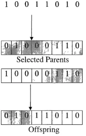
3.6 Crossover
one-point crossover and two -point crossover. One-point crossover is done by choosing two chromosomes as parents then choose a crossover point to make the exchange. The crossover point divides each chromosome into two halves and the exchange is executed by swapping one half of one chromosome with one half of the second chromosome. In two-point crossover, two crossover points are chosen then we exchange the two ends of one chromosome with the two ends of other chromosome. One point crossover can be executed as following:
1- Randomly select two chromosomes as parents 2- Generate a random number between 0 and 1
3- If the number is less than Pc, select a random crossover point and exchange the chromosomes beyond this point between the parents.
4- If the number is greater than Pc, the two parents are cloned to the next generation.
5- Repeat step 1 to step 5 until the whole population is reached. 1 0 0 1 1 0 1 0
0 1 0 0 j}; Xf- 1
"'04
Selected Parents
1 0 0
1
0 1 0
0 0 1
vwe
1
if
r
1 1 0 1 0
Offspring
3.7 Mutation
Mutation operation randomly changes an offspring after crossover operation and it occurs at low probability rate named mutation probability Pm. Mutation operation is the key operation to maintain diversity in genetic algorithm and prevents GA from being stuck at local optimal solution. Bit-flip mutation is the most common mutation operation in binary encoding. It is done by inverting ' 1 ' to'O' and '0' to ' 1 ' after passing a probability test on their position. In case they do not pass the bits remain unchanged.
Offspring 0 1 0
0 1 0
1 1 0 1 0
• "
0 1 0 1 0 Offspring after mutation
Figure (3.4) Mutation operation
3.8 Example
To demonstrate how GA works, we will try to find the maximum of
F(x) = x
1+x
2+x
3Start
I
Initialization
Fitness Evaluation
Crossover
Mutation
Fitness Evaluation
Step one. Initialization
In this step, we will initialize a random population of four chromosomes.
Each chromosome contains the initial value of the three variables in the
objective function x
x,x
2, and x
3. For simplicity, we will encode the three
variables in binary of four bits wordlength.
x , = l 0 0 0 1
x
2= 3 0 0 1 1
x
3= 0 0 0 0 0
To construct a chromosome, all three variables are concatenated
[0 0 0 1 0 0 1 1 0 0 0 0]
Now, we generate the full generation
Step Two. Fitness Evaluation
To get the fitness value of each chromosome, we decoded them to decimal then apply the fitness function as following:
Chromosomes Chi Ch2 Ch3 Ch4 0 0 0 1 0 0 1 0 0 1 1 0 1 0 0 1 0 0 0 0 0 1 0 1 1 0 0 0 1 0 1 0 0 0 0 1 0 1 0 0 0 0 1 1 0 1 0 0 Total fitness Fitness Values 4 11 9 23 47
The result of fitness evaluation
Step Three. Reproduction
In this example, we will use Roulette Wheel to select parents as following: 1-Sum up all fitness value 47.
2-Choose a random number between land 47 let us say 25.
Chromosomes Chi Ch2 Ch3 Ch4 0 0 0 1 0 0 1 0 0 1 1 0 1 0 0 1 0 0 0 0 0 1 0 1 1 0 0 0 1 0 1 0 0 0 0 1 0 1 0 0 0 0 1 1 0 1 0 0
Sum of the preceding Fitness
0+4=4
4+11=15
15+9=24
24+23=47
Sum of preceding fitness values
Since 47 is larger than the randomly selected number 24 and the fourth chromosome becomes the first chosen parent
Chi 1 0 0 1 0 1 0 0 1 0 1 0
The first selected parent We repeat steps 1-3 until the full population is reached. The second random number is 15
Chromosomes Chi Ch2 Ch3 Ch4 0 0 0 1 0 0 1 0 0 1 1 0 1 0 0 1 0 0 0 0 0 1 0 1 1 0 0 0 1 0 1 0 0 0 0 1 0 1 0 0 0 0 1 1 0 1 0 0
Sum of the preceding Fitness
0+4=4
4+11=15
15+9=24
Ch2 0 0 1 0 0 1 0 0 0 1 0 1
The second selected parent The third random number is 2
Chromosomes
Chi
Ch2
Ch3
Ch4 0
0
0
1 0
0
1
0 0
1
1
0 1
0
0
1 0
0
0
0 0
1
0
1 1
0
0
0 1
0
1
0 0
0
0
1 0
1
0
0 0
0
1
1 0
1
0
0
Sum of the preceding Fitness
0+4=4
4+11=15
15+9=24
24+23=47
So chromosome number one chosen and becomes the third parent
Ch3 0 0 0 1 0 0 1 1 0 0 0 0
The third selected parent
Chromosomes Chi Ch2 Ch3 Ch4 0 0 0 1 0 0 1 0 0 1 1 0 1 0 0 1 0 0 0 0 0 1 0 1 1 0 0 0 1 0 1 0 0 0 0 1 0 1 0 0 0 0 1 1 0 1 0 0
Sum of the preceding Fitness
0+4=4
4+11=15
15+9=24
24+23=47
So chromosome number two chosen and becomes the fourth parent
Ch4 0 0 1 0 0 1 0 0 0 1 0 1
The fourth selected parent
Step Four. Crossover
One-point crossover is used in this example as following:
1- Randomly select a pair of chromosomes to make the crossover operation. So we divide the population into pairs.
2- Choose a crossover probability Pc say 90% then generate a random number between [0 1] for each pair say [.6 .3]
Chi 0 0 0
W
Ch2 0 0 1
1 0 0 1 1 0 0 0 0
0 0 1 0 0 0 1 0 1
Crossover for the first and second chromosomes
Offspringl 0 0 0 0 0 1 0 0 0 1 0 1
First offspring
Offspring2 0 0 1 1 0 0 1 1 0 0 0 0
Ch3 0 1 1 0 0 0 0
Ch4 1 0 0 1 0 1 0
1 0 0 1 0
V
0 1 0 1 0
Crossover for the third and fourth chromosomes
Offspring3 0 1 1 0 0 0 0 1 1 0 1 0
Third offspring
Offspring4 1 0 0 1 0 1 0 0 0 0 1 0
So the new population is as following:
New nonulat ion of offsn rinp
Offspringl Offspring2 Offspring3 Offspring4 0 0 0 1 0 0 1 0 0 1 1 0 0 1 0 1 0 0 0 0 1 0 0 1 0 1 0 0 0 1 1 0 0 0 1 0 1 0 0 0 0 0 1 1 1 0 0 0 Decimal values XI 0 3 6 9 X2 4 3 1 4 X3 5 0 10 2
The resulting offspring
Step Five. Mutation
Offspringl Offspring2 Offspring3 Offspring4 0 0 0 1 0 0 1 0 0 1 1 0 0 1 0 1 0 0 0 0 1 0 0 1 0 1 0 0 0 1 1 0 0 0 1 0 1 0 0 0 0 0 1 1 1 0 0 0 8 3 6 9 4 3 0 12 5 0 10 2
V
Offspringl Offspring2 Offspring3 Offspring4 1 0 0 1 0 0 1 0 0 1 1 0 0 1 0 1 0 0 0 1 1 0 0 1 0 1 0 0 0 1 0 0 0 0 1 0 1 0 0 0 0 0 1 1 1 0 0 0Offspring after mutation
Step Six. Fitness Evaluation
The new population is decoded to decimal then evaluated by applying the
New nonnlat ion of offsn rincr Offspringl Offspring2 Offspring3 Offspring4 1 0 0 1 0 0 1 0 0 1 1 0 T 0 1 0 1 he c 0 0 0 1 eco 1 0 0 1 ded 0 1 0 0 0 1 0 0 offsprin 0 0 1 0 1 0 0 0 0 0 1 1 1 0 0 0 g population Decimal values XI 8 3 6 9 X2 4 3 0 12 X3 5 0 10 2 Chromosomes Offspringl Offspring2 Offspring3 Offspring4 1 0 0 1 0 0 1 0 0 1 1 0 0 1 0 1 0 0 0 1 1 0 0 1 0 1 0 0 0 1 0 0 0 0 1 0 1 0 0 0 0 0 1 1 1 0 0 0 Total fitness Fitness function 17 6 16 23 62
Fitness evaluation of offspring
3.9 GA Analysis
To understand the effects of GA operations, the schema notion has to be defined. A schema is a combination of a coding system of chromosomes and a 'do not care symbol' *. The do not care symbol * may take any value of the coding system for example let the binary system be the coding system So * can take 0 or 1. Let us have a four bit chromosome *1*0, this chromosome could be 0100, 0110, 1100, or 1110.
3.9.1 The Effect of Reproduction
Let H(Snt) represents the number of chromosomes of schema St. If Roulette Wheel is used, the number of chromosomes of the next schema can be estimated
H(S
l.*+l) = H ( S , . t ) x £ M
/ (S • ,t) is the average fitness of schema i .
f (t) is the average of the current schema.
If / (S • ,t) > 1 that means the schema has an above average fitness in the generation i and receive an increasing number of offspring in the next generation.
3.9.2 The Effect of Crossover Operation
A schema survives the crossover operation if the crossover point falls outside the schema length d(s). If one-point crossover is applied, the probability of a schema being destroyed is
L is the length of the chromosome So the probability of being survived is
P , ( s ) = l - P , ( s )
And by using the crossover probability P is
P
sc(s)>l-P
cxP,(s)
As result, the longer the schema is, the higher chance it will be destroyed.
3.9.3 The Effect of Mutation
A schema survives from distortion only if all positions in the schema remain unchanged. The survive probability is
P(s) = Pb°(s)
O(s) is the order of the schema
Pb is the probability of a single bit to survive P =1 -P
P is the mutation probability.
P(s)=l-P
mxO(s)
So the higher the order is, the higher the chance of a schema being
CHAPTER IV
DESIGN 2-D DIGITAL FILTERS BY SVD
4.1 Design recursive digital filters
The transfer function of a quadrantally symmetric filter has a separable
denominator H (z
{,Z
2) can be expressed as
k
H(z
l,z
2) = Yfi(Zi)8itei) (4.D
1=1
Let A = (a
lm) be a desired amplitude response where
a
lm=\H{e
jmi,e
]nvm)\, 1 < / < L , \<m<M
and let w
;and v
m, be normalized frequencies such that
I-I m - 1
u, = and v =
1
L-\
mM - 1
0 < u , < 1 , 0 < v ,
B< l
The singular value of A
r
A
= Z
ai
Ui
Vi (
4-
2>
/ = i
Where <J
lare the singular values of A.
u
iis the ith eigenvector of AA associated with the ith eigenvalue of.
V,. is the ith eigenvector of A A associated with CT .
r is the rank of A, and v, denotes the transpose of v
;. .
A
= Z ^
t?i
(4.3) = lWhere (/)l and y% are sets of orthogonal L-dimensional and M-dimensional vectors, respectively.
Now, by comparing (4.1 and 4.3) and assuming that k = 1, r=l and that
(j)x and yx are the desired amplitude responses for the 1-D filters characterized by f x( zx) and g1 ( z 2) respectively, a 2-D digital filter can
be designed as the following steps:
1- Design 1-D filters/, and g,, characterized by fx( zx) and g,( z2) by
using one of the many available optimization methods. 2- Connec t filters f t and gt, in cascade.
The transfer function of the cascade filter obtained is given by
Hl(zl,Z2)=fx(zx)gx(z2) (4.4) An important property of the SVD can be stated as
^-2>,r,'
i=i
= m m
A A
^-i»;
i=i
where d e R ,y e RL,and
\X =
L M
1=1 m=l
i l / 2
X Im
for 1 < k < r
LxM
is the Frobenius norm of a matrix X = (x , ) e R . The above relation
shows that for any fixed k (l<=k <= r), 7_^
(Y
tis a minimal
mean-square-(=1
error approximation to A. Since r >1, from Equation (4.5) can be written
A-H
x(e
jmi,e
J™
m) « A-(j)
xy
xFrom (4.6) A can be written as
A=(/)
xy
x+e
x(4.7)
If we compare (4.3) and (4.7), we get
=£,
(4.6)
*I=5>,K'
I=2
&=(/>
lY
l+Y
J<f>
lY
l1=2
The approximation error £
xis associated with the number of sections k that
have been realized. So S
xmay be reduced by finding a way of realizing
more of the terms in (4.3) by means of parallel filter sections so that we can
write
A=(/)
xy
x+(f)
1y
2+£
2where
r
i=3
Since all entries of A are nonnegative, it follows that all entries of
<f>x a n d Y\ a r e nonnegative. Nevertheless, the elements of 0t and yt
for i >= 2 may assume negative values so a careful treatment of
(f)2 and y2 is necessary to get red of their negative components. Let 02 and fl be the absolute values of the most negative components of (j)2 and y2 respectively. If
e , = [1 1 . . . 1]' E RL and ey = [1 1 . . . 1]' e RM
Then all components of
& = A + 02 £<* a n d fl = 72 + Yi2 ^ e (4.9)
are nonnegative. Let us assume that it is possible to design 1-D linear-phase or zero-phase filters characterized by
fi(z
x),g
x(z
2),f
2(zj), and g
2{z
2) such that
f,{e
]mi) = f
l(e
} l)
ja\ui1<1<L i=l,2
g>'
J W")=g
l(e""»)
, ; ^ / Ja2vl\<m<M i=l,2
7 ^ ,
g > ^ )
/1/77 'g
2(e
37Wm)
7
2mHere (j>2l and y2m are the Lth component of (j)2 and the mth component of y2 respectively, and CCX , OC2 are constants which are equal to zero if zero-phase filters are to be employed. Now let
ax = -7tnx and a2 = -7rn2
where nx , n2 are nonnegative integers, and define
f2(z
l)=f
2(z
l)-0
2zr
andg2(Zi) = g2(z2)-72Z -n
2
if we form
H
2(z
x,z
2)=f
x(z
x)g
x(z
2)+f
2(z
x)g
2(z
2)
(4.H)H2(ejmitejaVm)
= \fi(ejm" )gx{e]mm ) +f2(e"»l )g2{e]7tVm )
H A / ^ + ^ T U
l ^ ^ L , l<m<M
(4.12)
which in conjunction with (4.8) implies that
A
H2{e]7mi,e]7Wm)A-
0iY+027< A
- (fry + A7
2
)
=£n = m m<h ,71
, A A ' , A A '
A-tyn +<f>
27
2)
Evidently, the approximation error has been reduced from ex to e2 by means of a parallel subfilter. According to (4.13), the two-section 2-D digital filter obtained has an amplitude response which is a minimal mean-square-error approximation to the desired amplitude response.
Since / , ( z,) and g,( z2) corresponds to the largest singular value<7]m , the quantity fi(e}m'l)gx(ejm,m) represents the main contribution to the amplitude response of the 2-D filter. For this reason, the subfilter characterize / , ( z,) and g,( z2) is said to be the main section of the 2-D
filter. On the other hand, f2 (eJ m ) g 2 (eJ m m )
represents a correction to the amplitude response, and the subfilter characterized by / , ( z , ) and g , ( z2) is said to represent a correction
section.
Other correction sections characterized by / , ( z , ) and g, ( z2) can be
designed using (f)i a n d yi ( i = 3 , , k , k < r) in similar manner. When k sections are designed, including the main section,Z/^ (zx,z2) can be formed as
k
H
k(z
vz
2) = Y,f,^i)8
l(z
2)
1=1 Then we have
A - H
k(e
imii e i A-5>,K
< £. - minK A A
^-Z^
A
'
4.2 ERROR COMPENSATION
A further improvement is possible through the use of error compensation. When the main section and the correction sections are designed by using an optimization method, approximation errors will inevitably occur which will accumulate and manifest themselves as the overall approximation error in the design of the 2-D filter. Fortunately, it is possible to prevent the accumulation of error through compensation. When the design of the main section is complete, define an error matrix
E, = A - (4.15)
E2 — Ex = A
-and then perform SVD on El, to obtain
El =S2lA2722 +- + Sr20r27r2 (4A6>>
Data 0J2 and y22 can be used to deduce /2( z,) g2( z2)thus, the first
correction section can be designed. Now form error matrix E, as
S
22f
2(e
jmi)g
2(e
j™™)
f
x(e
j^)g
x(e
j^) + S
22f
2(e
jmi)g
2(e
j™™)
and perform SVD on E, to obtain
E
2=S
330
33y
33+... + S
r30
r3y
r3As before, data 033 and y3 can be used to design the second correction section. This procedure is continued until the elements of the error matrix become sufficiently small for the application at hand.
MZy)
-(g)—[~T|- * ~\~T
fllZt)
-0,
/ * < * , )
- 4
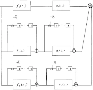
.?tc^>-4
Figure (4.1) Realization of quadrantally symmetric2-D filter
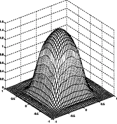
Example (1)
Design 4m order 2-D IIR low pass filter specified by:
H(e
j(0iri,e
j(O2T2)\=l
0 < ^a^+a^2 < 0A5x 0A5x < ^Jco^+ari < K.*t-.
N. X .
I
>i:
-i -i
i t h
14-
12-lllb
l l l l l
4.3 Design nonrecursive digital filters
The transfer function of a 2-D FIR filter with support in the rectangle
N. N.
defined by l- < n; < — - , i = 1,2can be written as
2 ' 2
Nl/ N2/
H(Z
X,Z
2)= X E h{n
vn
2)z-
xnxz
2ni(4.18)
N\/ N2/
Where h(n
x,n
2) is the impulse response. If h(n
x,n
2) is real and
h{n
x,n
2) = h(—n
x,—n
2)
Then the frequency response of the filter given by
Ny/ N
2/
H(z
x,z
2)= X Z M»i,«
2) «'
M H | r i« '
M B f 2= X ( ^ , 6 >2)
Is symmetrical with respect to the origin of (<^,£y2) plane such that
X (6)X,C02)=X {-G\,-(D2)
(4.19)
where -7t<o\,0)
2>7i
Assume the desired arbitrary frequency response A satisfies equation (4.19) that is:
X{n ul,7ivm) = X (-7T u^-n vm)