Institute of Statistics Mimeo Series No.2662
North Carolina State University, Raleigh, NC, USA
fastLASSO: Variable Selection in Kernel Machine Modeling for
2
Cross Disorder Analysis
Rachel Marceau*, Wenbin Lu*, Jin Szatkiewicz, and Jung-Ying Tzeng* §
4
1
Abstract
When trying to find genetic associations, traditional analyses follow a “bottom-up” approach,
6
examining one gene (or variant) and one disorder at a time, using meta analysis to combine
results for multiple genes/disorders. These approaches may be underpowered by ignoring
8
comorbidities of disorders and coheritability of variants and due to high multiple testing burden
of individual tests. We propose a “fastLasso” method to simultaneously analyze the effects
10
of multiple genes along a pathway on multiple diseases. In particular, we use a fast kernel
machine approach in conjunction with gene-level group lasso to pinpoint probable causal genes
12
within a pathway for a group of related phenotypes. Our approach takes advantage of shared
genetic risk between phenotypes, leading to increased power and better understanding of the
14
biological mechanism of shared disorders. Further, it is computationally efficient and flexible,
with support for both binary and continuous phenotypes, as well as for incorporation of data
16
from different individuals for the different disorders considered. We demonstrate the utility
and performance of our method over pathway-based single disorder analysis via simulation
18
study.
*Department of Statistics, North Carolina State University, Raleigh, North Carolina, United States of
Amer-ica
Department of Genetics, University of North Carolina at Chapel Hill, Chapel Hill, North Carolina, United
States of America
Bioinformatics Research Center, North Carolina State University, Raleigh, North Carolina, United States
of America
2
Introduction
20
2.1 Motivation for Cross Disorder Analysis
Pleiotropy, or the effect of one gene on multiple traits, is an important topic in statistical
22
genetics. Increasing evidence of comorbidity of diseases and of coheritability of variants that
are associated with given disorders suggests that we can gain a better understanding of the
24
genetic architecture of related disorders by considering them together within an analysis. This
increased understanding of gene multifunctionality can be used to improve detection, diagnosis,
26
classification, and treatment of correlated disorders (Hu et al., 2016; Insel et al., 2010; Lee
et al., 2012; Morris and Cuthbert, 2012; Sanislow et al., 2010). Data for multi-disorder studies
28
is also more widely available with electronic health data available to help quantify co-occuring
disorders (Hu et al., 2016), and multi-institution initiatives being created to better understand
30
shared disease pathology (e.g., NIMH’s Research Domain Criteria RDoC for studying related
psychological disorders (Insel et al., 2010; Morris and Cuthbert, 2012; Sanislow et al., 2010)).
32
A motivating example of related phenotypes includes the psychological disorders anorexia
nervosa (AN), schizophrenia (SCZ), and obsessive compulsive disorder (OCD), which evidence
34
suggests have a large proportion of shared heritability (between 40-60%) (Anttila et al., 2016)
and pairwise comorbidity much larger than the population prevalance of the individual
disor-36
ders (Achim et al., 2009; Buckley et al., 2008; Fawzi and Fawzi, 2012; Foulon, 2003; Godart
et al., 2000; G¨otestam et al., 1995; Hoff, 2012; Hudson et al., 2007; Kaye et al., 2004; Khalil
38
et al., 2011; Kouidrat et al., 2014; Lysaker and Whitney, 2009; Mukhopadhaya et al., 2009;
Poyurovsky et al., 2005, 2012; Rubenstein et al., 1992; Ruscio et al., 2010; Schirmbeck and
40
Zink, 2013; Seeman, 2014; Swinbourne et al., 2012; Yum et al., 2009). By studying all three
together, we can improve diagnosis and classification, making them more biologically-based
42
and the disorders themselves easier to detect (Insel et al., 2010; Morris and Cuthbert, 2012).
Li et al. (2014) discusses many other studies where leveraging pleiotropy can increase power,
44
e.g., for psychiatric disorders (Andreassen et al., 2013; of the Psychiatric Genomics
Consor-tium et al., 2013), cancer (Sakoda et al., 2013), and metabolic traits (Lee et al., 2012; Vattikuti
46
In addition to increasing our functional knowledge of pleiotropic effects, utilizing
informa-48
tion from multiple disorders simultaneously, as well as from multiple genes along a pathway,
can increase our signal to detect important genetic associations, as single-trait analyses ignore
50
shared information from correlated traits (Kiezun et al., 2012; Manolio et al., 2009) and can
have high multiple testing burden (Wang et al., 2015). The gain in power from multi-trait
52
analyses is especially important when dealing with variants with low effects and low minor
allele frequencies, which may be more difficult to detect, as is the case with rare variant
anal-54
ysis. Not only does incorporation of correlation phenotypes effectively increase the sample
size (Li et al., 2014; Maier et al., 2015), but leveraging coheritability information also enables
56
additional borrowing of signal.
2.2 Current Methods
58
Three main classes of methods currently exist to model multiple disorders simultaneously:
meta analysis and combined statistics, dimension reduction (e.g., principal component analysis,
60
canonical correlation analysis, similarity based), and multi-response regression (Galesloot et al.,
2014; Yang and Wang, 2012).
62
2.3 Meta Analysis and Combined Tests
Meta analyses and combined univariate tests are examples of “bottom-up” procedures, looking
64
at single genes and disorders individually, e.g., through univariate genome-wide association
studies (GWAS), and then combining results to detect pleiotropic effects and obtain tests of
66
association at a multi-trait level.
Examples of meta analyses/combined tests include the work of Andreassen et al. (2013);
68
Bolormaa et al. (2014); Van der Sluis et al. (2013); Yang et al. (2010). The approaches of both
Bolormaa et al. (2014) and Yang et al. (2010) create a vector of test statistics from univariate
70
association tests of a variant on a single trait and calculate a multivariate test statistic as a
function of these test statistics. They both aim to test the null hypothesis of no genetic effect
72
on any of the traits against the alternative that at least one trait has significant genetic effect
from the variant of interest.
Yang et al. (2010) assumes the vector of test statistics follows a multivariate normal
distri-bution and uses a modified O’Brien method (O’Brien, 1984; Wei and Johnson, 1985) to test
76
whether or not the mean of this distribution is equal to zero, i.e. whether there is any
associ-ation of the variant (or group of variants) with at least one of the traits. They create a test
78
statistic that is the linear combination of the multivariate normal means (and corresponding
estimated or known covariance of these means), estimating weights using sample splitting/cross
80
validation and obtain significance via resampling and permutation.
Bolormaa et al. (2014) creates a quadratic test statistic from the signed t-values from
82
GWAS (one for each variant of interest, if multiple variants are to be considered) and the
correlation between each pair of traits over all variants, which approximately follows a
chi-84
square distribution with degrees of freedom equal to the number of traits being considered.
Andreassen et al. (2013) and Van der Sluis et al. (2013) also look at summary statistic
86
data from univariate GWAS tests, but instead of test statistics focus on combining the
p-values. Andreassen et al. (2013) focuses on determining multivariate significance through the
88
conditional false discovery rate (FDR) of two traits. In particular, they used the p-values from
univariate GWAS tests to calculate the conditional cumulative distribution function (CDF) of
90
the (corrected) p-values for each trait, conditional on the nominal p-value from the other trait,
which they used to calculate the conditional FDR for each trait, creating a 2 dimensional “look
92
up” table, looking at the maximum of the two FDRs for each variant, which they compared
against a mixture model-based estimated distribution of SNPs (unconditional analysis). They
94
note their approach has merit because you would expect a higher likelihood of a true positive
variant association if it deemed significant in two associated phenotypes (Andreassen et al.,
96
2013). It is also nonparametric with few assumptions on the traits or genetic variants. However,
it does not extend to more than two traits like the aforementioned approaches.
98
Van der Sluis et al. (2013) combines univariate p-values for each trait into a “trait-based”
p-value in their TATES (Trait-Based Association Test that uses Extended Simes procedure)
100
approach, calculating the minimum p-value over all traits for a given variant, weighted by the
effective number of independent p-values. The effective number of p-values is calculated using
102
correlations between the traits. Again this is testing the null hypotheses of no association
104
between a particular variant and any of the traits. They note that follow-up is required to test
more specific hypotheses of the genotype-phenotype model.
106
Combined tests and meta analyses have the benefit that, because they only use summary
statistics (namely, the test statistic) from each GWAS test, they can analyze data with different
108
subjects (even using published data where subject-level data is not available) and with
dif-ferent types of traits together (e.g., quantitative, binary, and survival), without making many
110
assumptions on the distribution of the traits (Bolormaa et al., 2014; Van der Sluis et al., 2013;
Yang et al., 2010). Further, opposing effects of variants on different traits will not cancel each
112
other out to reduce power (Van der Sluis et al., 2013). In addition, the approaches of Yang
et al. (2010), Bolormaa et al. (2014), and Van der Sluis et al. (2013) can analyze an arbitrary
114
number of traits. However, these “bottom-up” methods may lose power by not taking into
account unified information, such as the comorbidity and coheritability of traits, that can be
116
incorporated by using the raw subject-level rather than summary data. These approaches also
lose power due to high multiple testing burden from performing separate tests for each genetic
118
variant (Wang et al., 2015). Finally, some, like Fisher’s method of combining test statistics,
can have inflated type I errors when traits are correlated (Aschard et al., 2014).
120
2.4 Dimension Reduction
Dimension reduction methods of multivariate analysis include principal component analysis
122
(PCA) and canonical correlation analysis (CCA). Rather than combining summary statistics,
dimension reduction approaches combine raw information, directly accounting for the
corre-124
lation between traits (Aschard et al., 2014). As such, they, along with multi-trait regression
methods, are examples of “top-down” approaches. These approaches take advantage of
com-126
bined information from multiple genes and/or phenotypes effectively performing meta analysis
at the start, then refining to localize significant associations.
128
Aschard et al. (2014) and Klei et al. (2008) use PCA to perform multi-trait analysis.
Aschard et al. (2014) suggests loss of power by only considering the top principal components
130
of variability in the phenotypes), and therefore proposes a global multistep combined PC
132
(mCPC) score. The CPC test statistic is a function of the cumulative distribution function
of the aggregate of tests of association between the leading PCs and genotype, and of the
134
aggregate of tests of association between the remaining PCs and genotype, and follows a
chi-square distribution under the null hypothesis. They note their method easily generalizes to
136
many traits, and can be used as part of a multivariate linear model to account for population
or family structure.
138
Klei et al. (2008) considers principal components of phenotype to not be biologically
ac-curate enough and proposes instead to look at tests for association between genotype and the
140
principal components of heritability (PCH). They create a new phenotype that is the linear
combination of the trait phenotypes that has the highest heritability (Klei et al., 2008). They
142
use sample splitting/bagging to estimate these optimal linear weights and note that they can
use this approach on residuals from PCs rather than the PCs themselves. They perform a test
144
of association between genotype and their PCH using a t-test.
Ferreira and Purcell (2008) use CCA to calculate a linear combination of traits that explains
146
the highest proportion of covariability between genotype and phenotype, as is implemented in
PLINK. MultiPhen (O’Reilly et al., 2012) is a similar method that is somewhat between
dimen-148
sion reduction and multi-trait regression models. MultiPhen performs an ordinal (proportional
odds logistic) regression, modeling the probability of the genetic variants being less than or
150
equal to a value (0,1,2) on a linear combination of the phenotypes, then using likelihood ratio
tests for each variant to test whether that variant is significantly associated with at least one
152
of the traits.
Dimension reduction techniques, again, can easily incorporate multiple (more than two)
154
traits and often have lower multiple testing burden than meta-analysis techniques. In addition,
they directly include correlations between traits, unlike meta analyses. However, they tend to
156
be applicable mostly to normal traits only, and are not able to combine traits. In addition,
they do not provide as interpretable results, as they relate linear combinations of traits with
158
2.5 Multi-trait Regression
160
Multi-trait regression approaches, like dimension reduction approaches, are “top-down”
ap-proaches, leveraging information about correlations between traits, comorbidity, and
coheri-162
tability directly. Most existing multi-trait regression models fit into the category of multivariate
linear mixed effects models.
164
2.5.1 Multivariate Linear Mixed Effects Models
Multivariate linear mixed effects models (multivariate LMMs, or mLMMs) have been commonly
166
used for genetic analyses involving multiple traits and multiple variants. mLMMs use a random
effects framework to explicitly model genetic sharing through the variance/covariance of a
168
genetic random effect term. Many mLMM methods focus on different aspects of multi-trait
analysis, such as estimating heritability and pleiotropy through the genetic correlation between
170
a set of traits (e.g., Korte et al. (2012); Lee et al. (2012); Loh et al. (2015); Vattikuti et al.
(2012)) and multivariate genetic risk prediction (e.g., Maier et al. (2015)).
172
Vattikuti et al. (2012) and Lee et al. (2012) proposed a bivariate LMM to estimate the
genetic correlation between a set of traits as a surrogate predictor of genome-wide pleiotropy.
174
Vattikuti et al. (2012) used an EM algorithm for restricted maximum likelihood (REML)
estimation for continuous traits, while Lee et al. (2012) proposed using an efficient average
176
information restricted maximum likelihood (AIREML) approach, approximating the Hessian
with the average information (Gilmour et al., 1995; Loh et al., 2015) to estimate on a continuous
178
scale, and showed how a liability threshold model could be used to obtain genetic correlation
when working with case/control data. Li et al. (2014), however, notes that the AIREML
180
algorithm occasionally fails to converge and is not ideal for binary traits as it uses normality
assumptions.
182
Loh et al. (2015) proposed “BOLT-REML” to increase efficiency and scalability (up to
50,000 subjects) of AIREML to estimate variance components and thus heritability and genetic
184
correlations, using Monte Carlo sampling to approximate the gradient for the mixed models.
They focus on common variants, however, and use liability scale to convert from case control
data.
Korte et al. (2012) proposed a multitrait mixed model (MTMM) to estimate genome-wide
188
heritability and genetic correlation of a pair of traits as functions of estimated variance
compo-nents of the model, taking into account relatedness/kinship of individuals and environmental
190
effects. They set up their model with two random effects terms to separately model
within-trait and between-within-trait effects (as an interaction between the within-trait an observation is for and
192
the genotype), allowing them to perform three marker-level tests for GWAS data, testing for:
(1) common and differing effect loci between traits, (2) common genetic effects between traits,
194
and (3) differing effects between traits. This model is more flexible but less efficient than that
proposed by Maier et al. (2015) for estimating pleiotropy, and only discusses testing for one
196
marker at a time for GWAS testing, which can have a high multiple testing burden.
Maier et al. (2015) proposed a mLMM for genetic risk prediction. Making use of the
198
AIREML approach, they calculate multi-trait genomic best linear unbiased predictors
(MT-GBLUPs) for individual risk prediction of sampled individuals and use these to calculate
200
snp-level BLUPs which can be projected to predict risk for individuals not in the sample.
Their approach allows for individuals to come from different samples, but has lower accuracy
202
for polygenic traits when not also incorporating additional gene annotation information.
While these approaches have been successful, their focus is not on association testing of
204
genotype with the traits, but on understanding and quantifying how the traits are related, or on
predicting phenotype for new individuals. Two approaches that do aim to perform association
206
testing are those of Zhou and Stephens (2014) and Casale et al. (2015).
Zhou and Stephens (2014) proposed a mLMM for GWAS, accounting for external covariates
208
such as population substructure and kinship, using the EM algorithm with Newton-Raphson
to combine stability and fast convergence. Their method does not allow for missingness in
210
phenotype data, however, and requires all phenotypes be measured on the same subject.
Fur-ther, they require a separate likelihood ratio test (LRT) for each variant of interest, leading to
212
a higher multiple testing burden.
Casale et al. (2015) proposed the multi-trait set test “mSet” model, using two variance
214
random effect) along with the combined genetic effect over a variant set (“set” random effect).
216
Their model allows for testing of no genetic effect (no “set” component) for genome-wide data
on up to 500,000 subjects using efficient linear algebra to make it take a similar amount of time
218
as fitting variance component models with a single variance component (Casale et al., 2015).
However, they do not pinpoint which variants within the set are more likely to be associated
220
with at least one of the phenotypes.
As mixed models, mLMMs are flexible and efficient, and are more robust and higher power
222
than fixed effects models for polygenic traits, as they can aggregate information over sets of
variants with weak individual effect (Korte et al., 2012; Wu et al., 2010, 2011). Like dimension
224
reduction approaches, they take advantage of shared information, coheritability and
comor-bidity, but yield much more interpretable results and may allow for phenotype data to come
226
from different individuals/studies. However, they assume normality of the phenotype data, or
simply perform a linearization of binary case/control data, which may work well for heritability
228
estimates (Lee et al., 2012) but is not valid for association testing because of poor modeling of
confounding effects.
230
2.6 Other Multi-trait Regression Models
Others have looked at non-LMM multi-trait regression models. Wang et al. (2015) proposed
232
a multivariate functional linear regression, which, rather than looking at the genetic loci as
discrete variables, includes their effects as a smooth function of genetic position. Approximate
234
F-tests, adjusting for covariates, then can be used to test for no genetic effect on any of the
traits of interest (Wang et al., 2015). This has the benefit of taking into account covariates and
236
genomic position and incorporating information on linkage disequilibrium in a natural manner,
but does not differentiate where the genetic signal, if any, is coming from.
238
Li et al. (2014) suggested the related bivariate ridge regression to predict multiple
phe-notypes, using the correlation between the diseases to increase prediction accuracy (the area
240
under the receiver operator curve) over single-trait models. They suggest that by effectively
increasing sample size, they can overcome one of the main bottlenecks in genetic risk prediction
242
param-eters for two disorders - one for each of the genetic effect of each disorder, and one for the
244
correlation between them, which they tune using a grid search and cross-validation to choose
the optimal values. Their use of ridge regression is due to the belief (De Los Campos et al.,
246
2010) that prediction models are more powerful with the inclusion of more traits with weaker
effects (even when including noise and opposite effect terms), e.g. a whole-genome model, than
248
a sparse model with only a few strong effects, as would be selected with a lasso model (Li et al.,
2014). This is good for risk prediction, but less ideal for pinpointing variants most likely to be
250
causal within a variant set.
Other approaches are similarity-based. Wei and Lu (2015) proposes a generalized similarity
252
U test for sequencing data that can be applied to multiple traits. Maity et al. (2012) and
Broadaway et al. (2016) propose kernel-based similarity methods. Maity et al. (2012) suggested
254
a multivariate kernel machine regression model, using a kernel term to express complex epistatic
effects of different variants. They use a score test statistic to test for no genetic effect of a set of
256
variants. This is similar to a mLMM, which can be seen through equivalence of norm functions
from the penalized log likelihood for a fixed covariance matrix, but can be generalized to
258
other exponential family distributions and allows more flexible modeling of relatedness between
traits. Broadaway et al. (2016) proposed the Gene Association with Multiple Traits (GAMuT),
260
which uses a “machine learning kernel distance-covariance” approach to test for association
between multiple traits and a set of genetic variants (Broadaway et al., 2016). Their approach
262
is nonparametric, relating the similarity between traits to the similarity between genotypes
on a pairwise level. It does not assume normality of phenotype, and is easy to include any
264
arbitrary number of genetic variants. However, neither of these methods focus on variant
selection of genetic variants that are associated with at least one trait.
266
2.7 Introduction to fastLasso
Following the work of Maity et al. (2012), we propose a kernel machine approach to look for
268
associations between genetic variants and a group of traits. Rather than testing for overall
association between a variant set and the traits, however, we wish to perform gene refining to
270
“fastLasso” method for performing cross-disorder variable selection on genes within a pathway.
272
Our method performs group lasso (Yuan and Lin, 2006) on an efficient decomposition of a
cross-disorder kernel matrix in order to identify which single nucleotide variants (SNVs) inside of
274
genes within a pathway are associated with at least one of multiple traits. We choose the
lasso rather than ridge regression, as in Li et al. (2014), for regularization because we wish
276
to pinpoint causal genes and generate hypotheses for further biological follow up, requiring
sparser and more defined models than are required for genetic risk prediction.
278
The fastLasso approach
1. takes advantage of the ability of kernel methods to capture complex epistatic relationships
280
between genetic variants,
2. is able to simultaneously perform effect estimation and variable selection on the SNVs
282
along a pathway for continuous or binary traits, and
3. can combine information from different studies, not requiring overlapping subjects for
284
the different traits considered.
By combining information from multiple disorders we have increased signal to detect rare
286
variants. We are able to do this in an efficient, scalable manner by borrowing the low-rank
fastKM decomposition of Marceau et al. (2015).
288
We perform a simulation study based off of the CoLaus genome wide association study
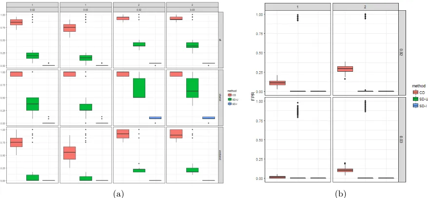
(GWAS) and exon-sequencing of single nucleotide variants (SNVs) to examine the performance
290
of our method compared with traditional approaches, only studying one disorder at a time,
then combining results.
292
3
Methods
We consider a study with D disorders of interest with some expected genetic or diagnostic
294
commonality. We let Yd denote a nd×1 vector of responses for all patients whose disease
status (continuous or binary phenotype) is known for disorderd= 1, ..., D. Further, we define
296
disorder d, and Gd,` to be a nd×m` genotype design matrix for gene ` = 1, ..., L within a
298
pathway of interest, wherem` is the total number of markers (single nucleotide variants, snvs)
genotyped for gene `.
300
For simplicity, we consider the case where we are interested inD= 3 coheritable disorders,
and letYn×1 = (Y1, Y2, Y3)T andXn×p =
X1 0 0 0 X2 0 0 0 X3
be the combined phenotype and covariate
302
design matrices, respectively. Heren=P3
d=1nd,p=
P3
d=1pd
Our goal is to determine which genes within a pathway of interest are significantly
as-304
sociated with at least one of the disorders, simultaneously performing variable selection and
estimating effect size from each variant/gene. To do this, we wish to perform group lasso based
306
on the cross-disorder kernel machine regression model
g(µY) =g
µY1 µY2 µY3
=β0+Xβ+
L
X
`=1
K`α` (1)
where βp×1 = (β1β2β3)T,µY =E(Y|X, G) is the phenotypic mean given all genetic and
non-308
genetic covariates, and g(µY) is the canonical link function. Further, K` is a n×n kernel
similarity matrix for gene ` and α` is a n×1 random effect of gene `, α` ∼ N(0, τ`K`−1) for
310
invertible K`, or more generally h` =K`α` ∼N(0, τ`K`).
In order to make this computationally feasible, we follow three main steps: (1) form a kernel
312
matrix to evaluate the genetic similarity between individuals within and between disorder
studies, (2) perform dimension reduction on the similarity kernel and form a low-rank fixed
314
effect term to summarize genetic effects over all studies/disorders, in the fastKM manner, and
(3) fit a fastLasso group lasso model using the low-rank fastKM term.
316
3.1 Kernel Evaluation
We form a kernel matrix to evaluate genetic similarity between all individuals using
column-318
standardized n×m` genotype design matrices, ˜G` = ( ˜G1,`,G˜2,`,G˜3,`)T, using the identity by
state (IBS) kernel or linear kernel ˜G`G˜T`. We note that for rare variants these are nearly
alent. We can alternatively expressK`in terms of its subcomponents: K` =
"K11,`K12,` K13,`
K12,`T K22,` K23,` KT 13,`K T 23,` K33,` # .
HereKd,d0,`isnd×nd0 matrix representing the genetic similarity between the individuals from 322
disorder/study dand disorder/study d0. This emphasizes the explicit incorporation of
covari-ance of variants between individuals from different studies (focusing on different disorders)
324
sinceKd,d0,` is not required to be zero.
3.2 Dimension Reduction
326
We wish to make group lasso computationally efficient for the large sample size and number
of variants. In order to do so, we perform kernel principal component analysis (kPCA) on our
328
Lkernel matrices. We perform an eigendecomposition of each kernel matrix as K` =Q`Λ`QT`,
where Q`,n×m` is a matrix of eigenvectors, and Λ`,m`×m` is a diagonal matrix of eigenvalues.
330
We then take the topkeigenvalues which collectively explain e% (e.g., 95%) of the variability
in the kernel matrix to form a rank-k decomposition, wherek < m`< n. Following the fastKM
332
methodology (Marceau et al., 2015), we can form a low rank approximation for the gene effect
as: (K`α`)n×1 ≈Z`Z`Tα` ≡(Z`γ`)k×1. We can thus form a new cross-disorder fastKM model
334
of the form
g(µY) =g
µY1 µY2 µY3
=β0+Xβ+
L
X
`=1
Z`γ` (2)
where γ` is a k`×1 vector, and k` << n, improving the computational efficiency, scalability,
336
and stability of a group lasso model fit.
3.3 fastLasso
338
We can can fit a group lasso model based on the cross-disorder fastKM model using existing
software, e.g. the grpreg package in R (Breheny and Huang, 2015), using the fastKM design
340
matrix Zn×(1+p+k)= (1, X, Z1, Z2, ..., ZL)T,k=PL`=1k` and cross-disorder phenotype vector
Y as input.
As a group lasso model, fastLasso solution is the γ that minimizes (Breheny and Huang,
2009)
344
Q(γ) = 1
2n||Y −Zγ|| 2
+λ
L
X
`=1
p
k`||γ`|| (3)
imposing sparsity on a pathway level, but borrowing signal from all variants within chosen
genes (Breheny and Huang, 2009).
346
We use Bayesian Information Criterion (BIC), BIC(λ) = 2Lλ + log(n)dfλ (Breheny and
Huang, 2009), to tune the regularization parameter λ, as BIC is known to be consistent and
348
computationally efficient (Yang, 2005). Heredfλ is the effective number of model parameters,
which in grpreg is estimated as a function of the fitted coefficients ˆγ and unpenalized fitted
350
coefficients (Breheny and Huang, 2009).
We obtain as output a list of the genes which are likely to be associated with at least one
352
of the traits, as well as relative effect sizes for the variants within those genes.
3.4 Computational Efficiency
354
The computational burden of the fastLasso approach is dominated by three operations: (1)
calculating the genetic similarity kernel matrices, (2) subsequently performing eigenvalue
de-356
composition on said kernel matrices, and (3) tuning and fitting a group lasso model. The first
two can be straightforwardly parallelized, as the separate gene kernel matrices are
indepen-358
dent from one another. We can further improve the efficiency of (2) by noting that the rank
of these similarity kernel matrices are always ≤ min(m`, n), so we can either compute just
360
the top m` eigenvalues for each kernel matrix (using efficient numerical linear algebra, as in
Qiu et al. (2016)), or equivalently perform eigendecomposition on the m` ×m` matrix ˜GTG˜
362
(we assume m` << n since each kernel matrix is gene-level). (3) is relatively efficient using
a fast coordinate descent algorithm in combination with the efficient BIC criterion (Breheny
364
4
Simulation Study
366
4.1 Data Generation
We perform a simulation study to examine the type I error and power of our method forD= 3
368
traits, using the CoLaus clinical trial study data of Firmann et al. (2008) as a basis to generate
simulated genotypes, using real data to take advantage of the natural correlations between
370
SNVs. The CoLaus study was a population-based trial examining cardiovascular,
psychologi-cal, and related metabolic risk factors in Caucasians in Lausanne, Switzerland (Firmann et al.,
372
2008; Preisig et al., 2009). From the initialn= 1769 individuals for which we have full
geno-type information (GWAS with imputations for missing genogeno-type information), we first form a
374
gene pool from which to base our simulations.
To do so, we extract information from genes within chromosomes 1-9 in the CoLaus study.
376
We are interested in how leveraging information from multiple disorders can help in the
iden-tification of rare variant associations, so we only include rare variants, which we here define as
378
having a minor allele frequency (MAF) of less than or equal to 1%, in our gene pool. Further,
we consider only those genes with at least 5 rare variants, leaving us with 5421 variants from
380
102 genes in our analysis, with between 5 and 230 SNVs per gene considered. The median
num-ber of rare variants/gene was 42. We perform sampling from this variant pool to form sampled
382
individuals and genotypes using random sampling for continuous traits, as described below.
An approach to perform case control sampling for binary traits can be found in appendix 6.
384
4.1.1 Random Sampling of Genotype Matrix
For continuous trait simulations, we perform random sampling of the variant pool. We first
386
create a 6000 x 5421 sample genotype matrixG∗, creating each individual genotype by
individ-ually sampling each gene with replacement from the genotypes from the original subjects, then
388
repeating this process 6000 times to get 6000 sampled genotypes. The first 2000 individuals
inG∗ were assigned to disorder 1, the next 2000 to disorder 2, and the last 2000 to disorder 3.
390
We randomly sample 20% of genes to be causal for one or more of the disorders. Of these,
we consider s = 40% or s = 60% of the causal variants to be common between all three
disorders and therefore 60% or 40% to be unique to only one of the disorders, spread evenly
amongst all three disorders. For simplicity, we consider all variants within causal genes to be
394
causal.
Continuous phenotypes for subjectsj= 1, ...,2000 within disorderd= 1,2,3 were randomly
396
generated from a normal distribution yj,d ∼N(µj,d,1) with meanµj,d = β0+XβX +G∗jdβd.
Here G∗jd denotes thed×jth row of the random genotype matrixG∗, i.e. the genotype for the
398
jth individual within disorder d.
For our simulations, we setβ0= 1 to approximate a 50% disease rate, and set
βd=
γG if gene`is causal for disorder d
0 if gene`is noncausal for disorderd
For simplicity, we do not consider any non-genetic covariates, so XβX = 0. Further, we
400
consider the same effect sizeγG for all causal genes within all disorders, rather than basing on
minor allele frequency. We consider γG = 1,2 for continuous traits, leading to models where
402
approximately 70% and 90% of the variability in the model is explained by the causal variants.
4.2 fastLasso Simulation
404
We use the grpreg package in R (Breheny and Huang, 2015) to perform group lasso on the
fastKM genetic design matrix, defining a group to be a gene. We find the optimal model over a
406
grid ofλtuning parameters using BIC, but further perform hard thresholding of the model to
obtain better separation of normed coefficients between causal and noncausal variants. This is
408
due to the properties of the null model fit, which still includes many nonzero coefficient terms,
likely due to the fact that the genotype design matrix is very rare. We use the null model
410
to determine an appropriate threshold, examining the distribution of the optimal fastLasso
coefficients. A histogram of the non-zero coefficients from this fit can be found in figure 1
412
below. We see that the largest absolute value coefficient is just over 0.03, indicating T = 0.02
andT = 0.03 are good choices for threshold values. To perform the hard thresholding, variants
414
zero.
416
Figure 1: Histogram of the non-zero coefficients from the null model fastLasso fit
We compare the cross-disorder model fit to that of fitting a group lasso separately within
each disorder. We summarize results from the single disorder analyses by determining the
418
union and intersection of the genes found to have non-zero coefficients over the three single
disorder model fits. These provide positive and negative controls, respectively.
420
5
Results
From table 1 below we see that in all simulated scenarios the cross disorder (CD) model is
422
able to find on average around double the causal genes that can be found using the union
of the single disorder (SD-U) approach. This is even more evident among the “unshared”
424
causal variants, i.e. those that are causal for a single disorder. While both methods do better
in finding the variants that are shared (i.e. causal for all three disorders), the magnitude of
426
improvement of the cross disorder model over the union of single disorder models is much larger
for unshared than shared variants. We see that the cross disorder model also outperforms the
428
union of single disorder models in terms of false positive rate, picking on average fewer
non-causal genes in the optimal model in all scenarios considered except for when γG = 2 and
430
T = 0.02. Though we see this trend, we note that the median false positive rate is actually
on average much lower for the single disorder models, indicating they may just choose fewer
432
This can be seen in figure 2 below. We note that with approximately 5000 genetic variants, a
434
model with sample sizen= 6000 is much more likely to be stable than one withn= 2000. The
intersect of the single disorder models performs poorly (has close to zero true positive rate) in
436
all scenarios, but also does not pick out any non-causal genes (i.e., a zero false positive rate)
and is overall of little interest statistically.
Table 1: Average true positive and false positive rates (and corresponding standard deviation) for cross disorder (CD), the union of single disorder (SD-U), and the intersection of single disorder (SD-I) continuous trait kernel machine model analyses over 100 simulations. Largest values within each category are in bold font.
True Positive Rate False Positive Rate
γG
% causal % variance
threshold shared unshared all
shared explained CD SD-U SD-I CD SD-U SD-I CD SD-U SD-I CD SD-U SD-I
1
40 66.8
0.02 1 0.52 0.01 0.68 0.2 0 0.81 0.33 0.004 0.1 0.18 0
(0) (0.25) (0.03) (0.08) (0.33) (0) (0.05) (0.3) (0.01) (0.03) (0.38) (0)
0.03 1 0.46 0.001 0.46 0.18 0 0.67 0.29 0 0.01 0.17 0
(0) (0.27) (0.01) (0.09) (0.33) (0) (0.06) (0.3) (0.01) (0.01) (0.35) (0)
60 69.4
0.02 0.93 0.42 0.004 0.81 0.23 0 0.88 0.33 0.002 0.12 0.2 0 (0.03) (0.31) (0.02) (0.1) (0.4) (0) (0.05) (0.35) (0.01) (0.04) (0.39) (0)
0.03 0.918 0.38 0.002 0.62 0.21 0 0.79 0.3 0.001 0.02 0.18 0 (0.01) (0.32) (0.01) (0.12) (0.39) (0) (0.05) (0.35) (0.01) (0.01) (0.36) (0)
2
40 88.8
0.02 1 0.81 0.11 0.87 0.38 0 0.92 0.55 0.04 0.28 0.25 0
(0) (0.16) (0.05) (0.05) (0.32) (0) (0.03) (0.24) (0.02) (0.05) (0.43) (0)
0.03 1 0.78 0.11 0.84 0.36 0 0.9 0.53 0.04 0.09 0.25 0
(0) (0.17) (0.05) (0.05) (0.31) (0) (0.03) (0.24) (0.02) (0.03) (0.42) (0)
60 90.1
0.02 0.94 0.5 0.08 0.98 0.22 0 0.96 0.38 0.048 0.3 0 0
(0.04) (0) (0) (0.04) (0) (0) (0.03) (0) (0) (0.04) (0) (0)
(a) (b)
Figure 2: True positive and false positive rates for cross disorder (CD), the union of single disorder (SD-U), and the intersection of single disorder (SD-I) continuous trait kernel machine model analyses over 100 simulations
6
Discussion
In this paper, we consider the benefits of leveraging information from multiple correlated traits
440
when conducting genetic association studies. Namely, we note that looking for association
between a set of variants and a set of phenotypes/disorders allows us to gain a better
under-442
standing of the underlying pleiotropy and true genetic architecture for these disorders, leading
to the potential for improved diagnosis, classification, and treatment. Further, by increasing our
444
effective sample size and by allowing incorporation of comorbidity and coheritability directly
into our analyses, we show that we increase our power to detect true causal variants (those that
446
are associated with at least one trait) while having nearly identical, or occasionally lower, false
positive rates. This additional power is especially helpful when trying to detect rare variant
448
associations.
While there are many existing approaches to incorporate multiple traits into an analysis,
450
not many are able to pinpoint the genes/variants most likely to be associated with at least one
trait. Most focus on either single-variant tests, which lead to high multiple testing burden, or
452
overall genome-wide tests of association. We propose the fastLasso method to efficiently perform
gene-selection while estimating relative effects of association between said genes and at least
454
one of the disorders that allows data to come from different studies, not requiring overlapping
individuals, in a way that is easy and valid to apply to both continuous and binary traits using
456
existing group lasso software. We note that as the number of genetic variants increases, it
becomes infeasible to perform this type of analysis without the fastKM decomposition.
458
In our simulations, we suggest using a hard threshold on fastLasso to decrease false positive
rates stemming from the sparse genotype design matrix. In our simulation we choose this
460
threshold using the null model fit, looking at the distribution of nonzero model coefficients. We
note that this could also be used for real data applications by fitting the fastLasso model with
462
permuted phenotype values, creating an effective null model for comparison.
While we focus on continuous trait SNV-level analysis for genetic main effects, we note it is
464
straightforward to extend to binary traits (also handled in the fastKM and grpreg R packages).
It is also straightforward to add terms to our model to incorporate other genetic information, e.g.
466
common single nucleotide polymorphisms (SNPs) and copy number variants (CNVs), leading to
a full pathway model to further understand the true biological network of the disorders studied.
468
Further, an additional kernel term could allow for incorporation of population substructure or
gene-environment (GxE) interaction, as is demonstrated in the fastKM methodology.
470
References
Achim, A. M., Maziade, M., Raymond, ´E., Olivier, D., M´erette, C., and Roy, M.-A. (2009).
472
How prevalent are anxiety disorders in schizophrenia? a meta-analysis and critical review on a significant association. Schizophrenia bulletin, 37(4):811–821.
474
Andreassen, O. A., Djurovic, S., Thompson, W. K., Schork, A. J., Kendler, K. S., O’Donovan,
M. C., Rujescu, D., Werge, T., van de Bunt, M., Morris, A. P., et al. (2013). Improved
476
detection of common variants associated with schizophrenia by leveraging pleiotropy with cardiovascular-disease risk factors. The American Journal of Human Genetics, 92(2):197–
478
209.
Anttila, V., Bulik-Sullivan, B., Finucane, H. K., Bras, J., Duncan, L., Escott-Price, V., Falcone,
480
G., Gormley, P., Malik, R., Patsopoulos, N., et al. (2016). Analysis of shared heritability in common disorders of the brain. bioRxiv, page 048991.
482
Aschard, H., Vilhj´almsson, B. J., Greliche, N., Morange, P.-E., Tr´egou¨et, D.-A., and Kraft, P. (2014). Maximizing the power of principal-component analysis of correlated phenotypes in
484
genome-wide association studies. The American Journal of Human Genetics, 94(5):662–676.
Bolormaa, S., Pryce, J. E., Reverter, A., Zhang, Y., Barendse, W., Kemper, K., Tier, B.,
486
Savin, K., Hayes, B. J., and Goddard, M. E. (2014). A multi-trait, meta-analysis for detecting pleiotropic polymorphisms for stature, fatness and reproduction in beef cattle.PLoS genetics,
488
10(3):e1004198.
Breheny, P. and Huang, J. (2009). Penalized methods for bi-level variable selection. Statistics 490
and its interface, 2(3):369.
Breheny, P. and Huang, J. (2015). Group descent algorithms for nonconvex penalized linear and
492
logistic regression models with grouped predictors. Statistics and computing, 25(2):173–187.
Broadaway, K. A., Cutler, D. J., Duncan, R., Moore, J. L., Ware, E. B., Jhun, M. A., Bielak,
494
L. F., Zhao, W., Smith, J. A., Peyser, P. A., et al. (2016). A statistical approach for testing cross-phenotype effects of rare variants. The American Journal of Human Genetics,
496
98(3):525–540.
Buckley, P. F., Miller, B. J., Lehrer, D. S., and Castle, D. J. (2008). Psychiatric comorbidities
498
and schizophrenia. Schizophrenia bulletin, 35(2):383–402.
Casale, F. P., Rakitsch, B., Lippert, C., and Stegle, O. (2015). Efficient set tests for the genetic
500
analysis of correlated traits. Nature methods, 12(8):755–758.
De Los Campos, G., Gianola, D., and Allison, D. B. (2010). Predicting genetic predisposition
502
in humans: the promise of whole-genome markers. Nature reviews. Genetics, 11(12):880.
Fawzi, M. H. and Fawzi, M. M. (2012). Disordered eating attitudes in egyptian antipsychotic
504
naive patients with schizophrenia. Comprehensive psychiatry, 53(3):259–268.
Ferreira, M. A. and Purcell, S. M. (2008). A multivariate test of association. Bioinformatics,
506
25(1):132–133.
Firmann, M., Mayor, V., Vidal, P. M., Bochud, M., P´ecoud, A., Hayoz, D., Paccaud, F.,
508
Preisig, M., Song, K. S., Yuan, X., et al. (2008). The colaus study: a population-based study to investigate the epidemiology and genetic determinants of cardiovascular risk factors and
510
metabolic syndrome. BMC cardiovascular disorders, 8(1):6.
Foulon, C. (2003). Schizophrenia and eating disorders. L’Encephale, 29(5):463–466.
512
Galesloot, T. E., Van Steen, K., Kiemeney, L. A., Janss, L. L., and Vermeulen, S. H. (2014). A comparison of multivariate genome-wide association methods. PloS one, 9(4):e95923.
514
Gilmour, A. R., Thompson, R., and Cullis, B. R. (1995). Average information reml: an efficient algorithm for variance parameter estimation in linear mixed models. Biometrics, pages 1440–
516
1450.
Godart, N. T., Flament, M. F., Lecrubier, Y., and Jeammet, P. (2000). Anxiety disorders in
518
anorexia nervosa and bulimia nervosa: co-morbidity and chronology of appearance. European Psychiatry, 15(1):38–45.
520
G¨otestam, K. G., Eriksen, L., and Hagen, H. (1995). An epidemiological study of eating disorders in norwegian psychiatric institutions. International Journal of Eating Disorders,
522
18(3):263–268.
Hoff, P. (2012). Eugen bleuler’s concept of schizophrenia and its relevance to present-day
524
psychiatry. Neuropsychobiology, 66(1):6–13.
Hu, J. X., Thomas, C. E., and Brunak, S. (2016). Network biology concepts in complex disease
526
comorbidities. Nature Reviews Genetics, 17(10):615–629.
Hudson, J. I., Hiripi, E., Pope, H. G., and Kessler, R. C. (2007). The prevalence and correlates
528
of eating disorders in the national comorbidity survey replication. Biological psychiatry, 61(3):348–358.
530
Insel, T., Cuthbert, B., Garvey, M., Heinssen, R., Pine, D. S., Quinn, K., Sanislow, C., and Wang, P. (2010). Research domain criteria (rdoc): toward a new classification framework for
532
research on mental disorders.
Kaye, W. H., Bulik, C. M., Thornton, L., Barbarich, N., and Masters, K. (2004). Comorbidity
534
of anxiety disorders with anorexia and bulimia nervosa. American Journal of Psychiatry, 161(12):2215–2221.
536
Khalil, R. B., Hachem, D., and Richa, S. (2011). Eating disorders and schizophrenia in male patients: a review. Eating and Weight Disorders-Studies on Anorexia, Bulimia and Obesity,
538
16(3):e150–e156.
Kiezun, A., Garimella, K., Do, R., Stitziel, N. O., Neale, B. M., McLaren, P. J., Gupta, N.,
540
Sklar, P., Sullivan, P. F., Moran, J. L., et al. (2012). Exome sequencing and the genetic basis of complex traits. Nature genetics, 44(6):623–630.
542
Klei, L., Luca, D., Devlin, B., and Roeder, K. (2008). Pleiotropy and principal components of heritability combine to increase power for association analysis. Genetic epidemiology,
544
32(1):9–19.
Korte, A., Vilhj´almsson, B. J., Segura, V., Platt, A., Long, Q., and Nordborg, M. (2012). A
546
mixed-model approach for genome-wide association studies of correlated traits in structured populations. Nature genetics, 44(9):1066–1071.
548
Kouidrat, Y., Amad, A., Lalau, J.-D., and Loas, G. (2014). Eating disorders in schizophrenia: implications for research and management. Schizophrenia research and treatment, 2014.
550
Lee, S. H., Yang, J., Goddard, M. E., Visscher, P. M., and Wray, N. R. (2012). Estimation of pleiotropy between complex diseases using single-nucleotide polymorphism-derived genomic
552
relationships and restricted maximum likelihood. Bioinformatics, 28(19):2540–2542.
Li, C., Yang, C., Gelernter, J., and Zhao, H. (2014). Improving genetic risk prediction by
554
leveraging pleiotropy. Human genetics, 133(5):639–650.
Loh, P.-R., Bhatia, G., Gusev, A., Finucane, H. K., Bulik-Sullivan, B. K., Pollack, S. J.,
556
de Candia, T. R., Lee, S. H., Wray, N. R., Kendler, K. S., et al. (2015). Contrasting genetic architectures of schizophrenia and other complex diseases using fast variance components
558
analysis. Nature genetics, 47(12):1385.
Lysaker, P. H. and Whitney, K. A. (2009). Obsessive–compulsive symptoms in schizophrenia:
560
prevalence, correlates and treatment. Expert review of neurotherapeutics, 9(1):99–107.
Maier, R., Moser, G., Chen, G.-B., Ripke, S., Coryell, W., Potash, J. B., Scheftner, W. A., Shi,
562
J., Weissman, M. M., Hultman, C. M., et al. (2015). Joint analysis of psychiatric disorders increases accuracy of risk prediction for schizophrenia, bipolar disorder, and major depressive
564
disorder. The American Journal of Human Genetics, 96(2):283–294.
Maity, A., Sullivan, P., and Tzeng, J. (2012). Multivariate phenotype association analysis by
566
marker-set kernel machine regression. Genet. Epidemiol., 36(7):686–695.
Makowsky, R., Pajewski, N. M., Klimentidis, Y. C., Vazquez, A. I., Duarte, C. W., Allison,
568
D. B., and de Los Campos, G. (2011). Beyond missing heritability: prediction of complex traits. PLoS genetics, 7(4):e1002051.
570
Manolio, T. A., Collins, F. S., Cox, N. J., Goldstein, D. B., Hindorff, L. A., Hunter, D. J., McCarthy, M. I., Ramos, E. M., Cardon, L. R., Chakravarti, A., et al. (2009). Finding the
572
missing heritability of complex diseases. Nature, 461(7265):747–753.
Marceau, R., Lu, W., Holloway, S., Sale, M. M., Worrall, B. B., Williams, S. R., Hsu, F.-C.,
574
and Tzeng, J.-Y. (2015). A fast multiple-kernel method with applications to detect gene-environment interaction. Genetic epidemiology, 39(6):456–468.
576
Morris, S. E. and Cuthbert, B. N. (2012). Research domain criteria: cognitive systems, neural circuits, and dimensions of behavior. Dialogues in clinical neuroscience, 14(1):29.
578
Mukhopadhaya, K., Krishnaiah, R., Taye, T., Nigam, A., Bailey, A., Sivakumaran, T., and Fineberg, N. (2009). Obsessive-compulsive disorder in uk clozapine-treated schizophrenia
580
and schizoaffective disorder: a cause for clinical concern. Journal of Psychopharmacology, 23(1):6–13.
582
O’Brien, P. C. (1984). Procedures for comparing samples with multiple endpoints. Biometrics, pages 1079–1087.
584
of the Psychiatric Genomics Consortium, C.-D. G. et al. (2013). Identification of risk loci with shared effects on five major psychiatric disorders: a genome-wide analysis. The Lancet,
586
381(9875):1371–1379.
O’Reilly, P. F., Hoggart, C. J., Pomyen, Y., Calboli, F. C., Elliott, P., Jarvelin, M.-R., and
588
Coin, L. J. (2012). Multiphen: joint model of multiple phenotypes can increase discovery in gwas. PloS one, 7(5):e34861.
590
Poyurovsky, M., Weizman, R., Weizman, A., and Koran, L. (2005). Memantine for treatment-resistant ocd. American journal of psychiatry, 162(11):2191–a.
592
Poyurovsky, M., Zohar, J., Glick, I., Koran, L. M., Weizman, R., Tandon, R., and Weizman, A. (2012). Obsessive-compulsive symptoms in schizophrenia: implications for future psychiatric
594
classifications. Comprehensive psychiatry, 53(5):480–3.
Preisig, M., Waeber, G., Vollenweider, P., Bovet, P., Rothen, S., Vandeleur, C., Guex, P.,
596
Middleton, L., Waterworth, D., Mooser, V., et al. (2009). The psycolaus study: methodology and characteristics of the sample of a population-based survey on psychiatric disorders and
598
their association with genetic and cardiovascular risk factors. BMC psychiatry, 9(1):9.
Qiu, Y., Mei, J., and authors of the ARPACK library. See file AUTHORS for details. (2016).
600
rARPACK: Solvers for Large Scale Eigenvalue and SVD Problems. R package version 0.11-0.
Rubenstein, C. S., Pigott, T. A., L’Heureux, F., Hill, J. L., and Murphy, D. (1992). A
prelimi-602
nary investigation of the lifetime prevalence of anorexia and bulimia nervosa in patients with obsessive compulsive disorder. The Journal of clinical psychiatry.
604
Ruscio, A., Stein, D., Chiu, W., and Kessler, R. (2010). The epidemiology of obsessive-compulsive disorder in the national comorbidity survey replication. Molecular psychiatry,
606
15(1):53.
Sakoda, L. C., Jorgenson, E., and Witte, J. S. (2013). Turning of cogs moves forward findings
608
for hormonally mediated cancers. Nature genetics, 45(4):345–348.
Sanislow, C. A., Pine, D. S., Quinn, K. J., Kozak, M. J., Garvey, M. A., Heinssen, R. K., Wang,
610
P. S.-E., and Cuthbert, B. N. (2010). Developing constructs for psychopathology research: research domain criteria. Journal of abnormal psychology, 119(4):631.
612
Schirmbeck, F. and Zink, M. (2013). Comorbid obsessive-compulsive symptoms in schizophre-nia: contributions of pharmacological and genetic factors. Frontiers in pharmacology, 4.
614
Seeman, M. V. (2014). Eating disorders and psychosis: Seven hypotheses. World journal of psychiatry, 4(4):112.
616
Swinbourne, J., Hunt, C., Abbott, M., Russell, J., St Clare, T., and Touyz, S. (2012). The comorbidity between eating disorders and anxiety disorders: Prevalence in an eating
disor-618
der sample and anxiety disorder sample. Australian & New Zealand Journal of Psychiatry, 46(2):118–131.
620
Van der Sluis, S., Posthuma, D., and Dolan, C. V. (2013). Tates: efficient multivariate genotype-phenotype analysis for genome-wide association studies. PLoS genetics, 9(1):e1003235.
622
Vattikuti, S., Guo, J., and Chow, C. C. (2012). Heritability and genetic correlations explained by common snps for metabolic syndrome traits. PLoS genetics, 8(3):e1002637.
624
Wang, Y., Liu, A., Mills, J. L., Boehnke, M., Wilson, A. F., Bailey-Wilson, J. E., Xiong, M., Wu, C. O., and Fan, R. (2015). Pleiotropy analysis of quantitative traits at gene level by
626
multivariate functional linear models. Genetic epidemiology, 39(4):259–275.
Wei, C. and Lu, Q. (2015). A generalized similarity u test for multivariate analysis of sequencing
628
data. arXiv preprint arXiv:1505.01179.
Wei, L. and Johnson, W. E. (1985). Combining dependent tests with incomplete repeated
630
measurements. Biometrika, 72(2):359–364.
Wray, N. R., Yang, J., Hayes, B. J., Price, A. L., Goddard, M. E., and Visscher, P. M. (2013).
632
Pitfalls of predicting complex traits from snps. Nature reviews. Genetics, 14(7):507.
Wu, M., Kraft, P., Epstein, M., Taylor, D., Chanock, S., Hunter, D., and Lin, X. (2010).
634
Powerful SNP-set analysis for case-control genome-wide association studies. Am. J. Hum. Genet., 86(6):929–942.
636
Wu, M., Lee, S., Cai, T., Li, Y., Boehnke, M., and Lin, X. (2011). Rare-variant association testing for sequencing data with the sequence kernel association test. Am. J. Hum. Genet.,
638
89(1):82–93.
Yang, Q. and Wang, Y. (2012). Methods for analyzing multivariate phenotypes in genetic
640
association studies. Journal of probability and statistics, 2012.
Yang, Q., Wu, H., Guo, C.-Y., and Fox, C. S. (2010). Analyze multivariate phenotypes in
642
genetic association studies by combining univariate association tests. Genetic epidemiology, 34(5):444–454.
644
Yang, Y. (2005). Can the strengths of aic and bic be shared? a conflict between model indentification and regression estimation. Biometrika, 92(4):937–950.
646
Yuan, M. and Lin, Y. (2006). Model selection and estimation in regression with grouped vari-ables. Journal of the Royal Statistical Society: Series B (Statistical Methodology), 68(1):49–
648
67.
Yum, S. Y., Caracci, G., and Hwang, M. Y. (2009). Schizophrenia and eating disorders. Psy-650
chiatric Clinics of North America, 32(4):809–819.
Zhou, X. and Stephens, M. (2014). Efficient multivariate linear mixed model algorithms for
652
genome-wide association studies. Nature methods, 11(4):407–409.
Appendices
654
A Case Control Sampling of Genotype Matrix for Binary Traits
Below we discuss a case control framework for binary trait simulations for multiple traits that
656
enables true controls (i.e., individuals who are cases for all of the considered traits). We note
the model fitting would be the same as for quantitative traits using the generalized model
658
framework.
Given the randomly sampled genotype matrix G∗, we consider a case control sampling
660
framework to generate simulated genotype and phenotype for all three disorders, giving us
CSd = 1000 cases for each disorder d = 1,2,3 and CN = 3000 “true controls,” defined as
662
those which are controls for all three disorders simultaneously – 1000 per disorder. Here causal
variants are determined in the same manner as for continuous phenotype simulations.
664
1. Sample one individual (row) from G∗, which we denote as G∗i.
2. For disorderd= 1,2,3 do:
666
(a) If number of accumulated sampled cases for disorderdis less than the desired number
of cases, or if the number of true controls is less than the desired number of controls:
668
i. Generate probability of case for individuali, disorderdas: pi,d=
exp(β0+XβX+G∗
iβd)
1+exp(β0+XβX+G∗
iβd)
ii. Generate phenotype for individuali, disorder das: yi,d ∼Bin(1, pi,d).
670
iii. If yi,d = 1, save individual i as a case for disorder d, and sample the next
individual. Otherwise, continue.
672
3. Ifyi,d = 0 ∀d, save individual ias a true control.
4. Continue until all cases and controls are determined.
674
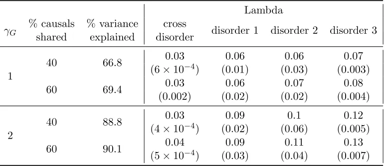
B Cross Disorder and Single Disorder Tuning Parameter Summaries
Table 2: Average optimal tuning parameter (and corresponding standard deviation) for the cross disorder and single disorder continuous trait kernel machine models over 100 simulations
Lambda
γG
% causals % variance cross
disorder 1 disorder 2 disorder 3 shared explained disorder
1
40 66.8 0.03 0.06 0.06 0.07
(6×10⁻⁴) (0.01) (0.03) (0.003)
60 69.4 0.03 0.06 0.07 0.08
(0.002) (0.02) (0.02) (0.004)
2
40 88.8 0.03 0.09 0.1 0.12
(4×10⁻⁴) (0.02) (0.06) (0.005)
60 90.1 0.04 0.09 0.11 0.13
(5×10⁻⁴) (0.03) (0.04) (0.007)