Scholarship at UWindsor
Scholarship at UWindsor
Electronic Theses and Dissertations Theses, Dissertations, and Major Papers
Winter 2014
Sparse machine learning models in bioinformatics
Sparse machine learning models in bioinformatics
Yifeng Li
University of Windsor
Follow this and additional works at: https://scholar.uwindsor.ca/etd
Recommended Citation Recommended Citation
Li, Yifeng, "Sparse machine learning models in bioinformatics" (2014). Electronic Theses and Dissertations. 5023.
https://scholar.uwindsor.ca/etd/5023
This online database contains the full-text of PhD dissertations and Masters’ theses of University of Windsor students from 1954 forward. These documents are made available for personal study and research purposes only, in accordance with the Canadian Copyright Act and the Creative Commons license—CC BY-NC-ND (Attribution, Non-Commercial, No Derivative Works). Under this license, works must always be attributed to the copyright holder (original author), cannot be used for any commercial purposes, and may not be altered. Any other use would require the permission of the copyright holder. Students may inquire about withdrawing their dissertation and/or thesis from this database. For additional inquiries, please contact the repository administrator via email
YIFENG LI
A Dissertation
Submitted to the Faculty of Graduate Studies through the School of Computer Science in Partial Fulfillment of the Requirements for
the Degree of Doctor of Philosophy at the University of Windsor
Windsor, Ontario, Canada 2013
c
YIFENG LI
APPROVED BY:
F. Wu, External Examiner
Department of Mechanical Engineering, University of Saskatchewan
R. Caron, Outside Department Reader Department of Mathematics and Statistics
R. Gras, Department Reader School of Computer Science
R. Kent, Department Reader School of Computer Science
L. Rueda, Co-Advisor School of Computer Science
A. Ngom, Advisor
School of Computer Science
Previous Publication
I
Co-Authorship Declaration
I hereby declare that this thesis incorporates material that is result of joint research, as
follows:
1. The decomposition method for sparse coding, covered in Chapter 2, is my work in collaboration with Professor R.J. Caron. The work is described in paper [Y. Li, R.J.
Caron, and A. Ngom, “A decomposition method for large-scale sparse coding in
rep-resentation learning,” IEEE World Congress in Computational Intelligence (WCCI),
July 2014, to be submitted.]. Y. Li proposed the initial idea, implemented it, and
wrote the draft of the paper. Y. Li conducted the experiments with the guidance of Professors R. Caron. Dr. R. Caron also evaluated the theoretical soundness of this
idea. All authors contributed to the final version of this paper.
2. The hierarchical model, described in Chapter 5, stems from the decision-tree based multi-class pair-wise strategy for linear dimensionality reduction and classification,
proposed in [L. Rueda, B.J. Oommen, and C. Henriquez, “Multi-class pairwise
lin-ear dimensionality reduction using heteroscedastic schemes,” Pattern Recognition, vol.
43, no. 7, pp. 2456 - 2465, 2010.]. The difference between the former and the
lat-ter is that the former learns the tree structure based on a one-versus-rest scheme,
while the latter based on a pair-wise scheme. We applied the hierarchical model in
[I. Rezaeian, Y. Li, M. Crozier, E. Andrechek, A. Ngom, L. Rueda, and L. Porter,
“Identifying informative genes for prediction of breast cancer subtypes,” IAPR
Inter-national Conference on Pattern Recognition in Bioinformatics (PRIB), Nice, June,
2013, LNBI 7986, pp. 138-148.] to identify the gene bio-markers of breast cancer
sub-types, under the supervision of Professors A. Ngom, L. Rueda, and L. Porter. In this
collaborative work, all authors contribute to the formulation of the hierarchical model.
Furthermore, Y. Li wrote the draft of the introduction, method, biological analysis,
and conclusions, I. Rezaeian surveyed the related work, conducted the experiments in Weka and wrote the experimental part. The rest of authors proof-read the paper.
In this dissertation, I re-implemented the hierarchical model in MATLAB, and redid
the experiments using my own implementations of linear models in the environment of MATLAB.
3. The nearest-border technique, covered in Chapter 5, is the outcome of our joint
research with Dr. B.J. Oommen with Carleton University, Ottawa. This
prelim-inary work has been accepted as [Y. Li, B.J. Oommen, A. Ngom, and L. Rueda, “A new paradigm for pattern classification: Nearest border techniques,” 26th
Aus-tralasian Joint Conference on Artificial Intelligence, New Zealand, Dec. 2013, pp.
441-446.]. Y. Li devised the nearest-border concepts, implemented them in
MAT-LAB, conducted the experiment, and wrote the draft of the methodology, under the
supervision of Professors B.J. Oommen, A. Ngom, and L. Rueda. B.J. Oommen
an-alyzed the experimental results, wrote the introduction and related work parts, and significantly polished the paper.
4. In Chapter 6, the time-series spectral clustering method is a joint work with Dr. A.
Ngom, L. Rueda, and N. Subhani, published as [Y. Li, N. Subhani, A. Ngom, and L.
Rueda, ”Alignment-based versus variation based transformation methods for clustering microarray time-series data,” ACM International Conference On Bioinformatics and
Computational Biology (BCB), Niagara Falls, NY, Aug. 2010, pp.53-61.]. The idea of
using spectral clustering was proposed by Professors A. Ngom. Professor A. Ngom also designed the algorithm. Y. Li implemented the methods including spectral clustering,
variation-based data transformation, and the new clustering validation index. Y. Li
also conducted the computational experiments in MATLAB. N. Subhani, draw the figures and computed the accuracy. A. Ngom wrote the draft of the paper. All
the authors contributed the final version of this paper. Professor L. Rueda is the
earliest contributor of the multiple alignment theory [L. Rueda, A. Bari, and A. Ngom, ”Clustering time-series gene expression data with unequal time intervals,” Springer
Trans. on Compu. Systems Biology X, vol. 10, no. 1974, pp. 100-123, 2008.].
5. In Chapter 7, Professor A. Ngom contributes to the theory and algorithm of
regula-tory networks from time-series microarray data,” IEEE Symposium on Computational
Intelligence in Bioinformatics and Computational Biology (CIBCB/SSCI), Singapore,
Apr. 2013, pp. 83-90.]. Y. Li implemented the algorithm, and did experiment on
artificial data and some real-life data. Y. Li wrote the draft of the above paper, and
Professor A. Ngom contributed to the final version. The experiment on real-life data
and sensitivity analysis were conducted by Dr. H. Chen and J. Zheng of National Technological University, Singapore, in order to test the performance of our
MMHO-DBN method. We are working on a journal paper to be submitted to Journal of
Computational Biology in October.
6. In Chapter 8, the main theory and algorithm of the imputation methods proposed in
[Y. Li, A. Ngom, and L. Rueda, “Missing value imputation methods for
gene-sample-time microarray data analysis,” IEEE Symposium on Computational Intelligence in
Bioinformatics and Computational Biology (CIBCB), Montreal, Canada, May 2010,
pp.183-189.], is contributed by Professor A. Ngom. Y. Li did literature survey,
imple-mented the algorithms, conducted experiments, and wrote the first draft of the paper.
A. Ngom contributed to the final version of this paper.
I am aware of the University of Windsor Senate Policy on Authorship and I certify that
I have properly acknowledged the contribution of other researchers to my thesis, and have
obtained written permission from each of the co-author(s) to include the above material(s) in my thesis.
II
Declaration of Previous Publication
This thesis includes 18 original papers that have been previously published/submitted for
publication in peer reviewed journals and conference proceedings, as follows:
Thesis ChapterPublication Title/Full Citation Publication Status Chapter 2 Y. Li and A. Ngom, “Classification approach based on non-negative
least squares,”Neurocomputing, vol. 118, pp. 41-57, 2013.
published
Chapter 2 Y. Li and A. Ngom, “Sparse representation approaches for the classification of high-dimensional biological data,” BMC Systems Biology, vol. 7, no. Suppl 4, pp. S6, 2013.
published
Chapter 2 Y. Li and A. Ngom, “Non-negative least squares methods for the classification of high dimensional biological data,” IEEE/ACM Transactions on Computational Biology and Bioinformatics, vol. 10, no. 2, pp. 447-456, 2013.
Chapter 2 Y. Li and A. Ngom, “Fast sparse representation approaches for the classification of high-dimensional biological data,”IEEE Inter-national Conference on Bioinformatics and Biomedicine (BIBM), Philadelphia, Oct. 2012, pp. 306-311.
published
Chapter 2 Y. Li and A. Ngom, “A new kernel non-negative matrix factoriza-tion and its applicafactoriza-tion in microarray data analysis,”IEEE Sympo-sium on Computational Intelligence in Bioinformatics and Compu-tational Biology (CIBCB), San Diego, CA, May 2012, pp. 371-378.
published
Chapter 2 Y. Li and A. Ngom, “Fast kernel sparse representation approaches for classification,”IEEE International Conference on Data Mining (ICDM), Brussels, Belgium, Dec. 2012, pp. 966-971.
published
Chapter 2 Y. Li and A. Ngom, “Supervised dictionary learning via non-negative matrix factorization for classification,”International Con-ference on Machine Learning and Applications (ICMLA), Boca Ra-ton, Florida, Dec. 2012, pp. 439-443.
published
Chapter 2 Y. Li and A. Ngom, “Versatile sparse matrix factorization and its applications in high-dimensional biological data analysis,” IAPR International Conference on Pattern Recognition in Bioinformatics
(PRIB), Nice, June, 2013, LNBI 7986, pp. 91-101.
published
Chapter 2 Y. Li, “Sparse representation for machine learning,”26th Canadian Conference on Artificial Intelligence (AI 2013), Regina, May, 2013, LNAI 7884, pp. 352-357.
published
Chapter 2 Y. Li, R.J. Caron, and A. Ngom, “A decomposition method for large-scale sparse coding in representation learning,”IEEE World Congress in Computational Intelligence (WCCI), July 2014.
in preparation
Chapter 3 Y. Li and A. Ngom, “The non-negative matrix factorization toolbox for biological data mining,” BMC Source Code for Biology and Medicine, vol. 8, pp. 10, 2013.
published
Chapter 4 Y. Li and A. Ngom, “Classification of clinical gene-sample-time microarray expression data via tensor decomposition methods,”
LNBI/LNCS: Selected Papers of 2010 International Meeting on
Computational Intelligence Methods for Bioinfomatics and Bio-statistics (CIBB), vol. 6685, pp. 275-286, 2011.
published
Chapter 4 Y. Li and A. Ngom, “Mining gene-sample-time microarray data,” in L. Rueda ed. Microarray Image and Data Analysis: Theory and Practice, CRC Press/Taylor & Francis, Dec. 2013.
in press
Chapter 4 Y. Li and A. Ngom, “Classification approach based on non-negative least squares,”Neurocomputing, vol. 118, pp. 41-57, 2013.
Chapter 5 Y. Li, B.J. Oommen, A. Ngom, and L. Rueda, “A new paradigm for pattern classification: nearest border techniques,” 26th Aus-tralasian Joint Conference on Artificial Intelligence, New Zealand, Dec. 2013, pp. 441-446.
in press
Chapter 5 I. Rezaeian, Y. Li, M. Crozier, E. Andrechek, A. Ngom, L. Rueda, and L. Porter, “Identifying informative genes for prediction of breast cancer subtypes,” IAPR International Conference on Pat-tern Recognition in Bioinformatics (PRIB), Nice, June, 2013, LNBI 7986, pp. 138-148.
published
Chapter 6 Y. Li, N. Subhani, A. Ngom, and L. Rueda, ”Alignment-based ver-sus variation based transformation methods for clustering microar-ray time-series data,” ACM International Conference On Bioin-formatics and Computational Biology (BCB), Niagara Falls, NY, Aug. 2010, pp.53-61.
published
Chapter 7 Y. Li and A. Ngom, “The max-min high-order dynamic Bayesian network learning for identifying gene regulatory networks from time-series microarray data,” IEEE Symposium on Computa-tional Intelligence in Bioinformatics and ComputaComputa-tional Biology
(CIBCB/SSCI), Singapore, Apr. 2013, pp. 83-90.
published
Chapter 8 Y. Li and A. Ngom, “Mining gene-sample-time microarray data,” in L. Rueda ed. Microarray Image and Data Analysis: Theory and Practice, CRC Press/Taylor & Francis, Dec. 2013.
in press
Chapter 8 Y. Li, A. Ngom, and L. Rueda, “Missing value imputation meth-ods for gene-sample-time microarray data analysis,” IEEE Sympo-sium on Computational Intelligence in Bioinformatics and Compu-tational Biology (CIBCB), Montreal, Canada, May 2010, pp.183-189.
published
Chapter 8 Y. Li and A. Ngom, “Classification approach based on non-negative least squares,”Neurocomputing, vol. 118, pp. 41-57, 2013.
published
I certify that I have obtained a written permission from the copyright owner(s) to include
the above published material(s) in my thesis. I certify that the above material describes work completed during my registration as graduate student at the University of Windsor.
I declare that, to the best of my knowledge, my thesis does not infringe upon anyone’s
copyright nor violate any proprietary rights and that any ideas, techniques, quotations, or any other material from the work of other people included in my thesis, published or
Furthermore, to the extent that I have included copyrighted material that surpasses the
bounds of fair dealing within the meaning of the Canada Copyright Act, I certify that I
have obtained a written permission from the copyright owner(s) to include such material(s) in my thesis.
I declare that this is a true copy of my thesis, including any final revisions, as approved
The meaning of parsimony is twofold in machine learning: either the structure or (and) the
parameter of a model can be sparse. Sparse models have many strengths. First, sparsity is an important regularization principle to reduce model complexity and therefore avoid
overfitting. Second, in many fields, for example bioinformatics, many high-dimensional
data may be generated by a very few number of hidden factors, thus it is more reasonable to use a proper sparse model than a dense model. Third, a sparse model is often easy to
interpret. In this dissertation, we investigate the sparse machine learning models and their applications in high-dimensional biological data analysis. We focus our research on five
types of sparse models as follows.
First, sparse representation is a parsimonious principle that a sample can be approxi-mated by a sparse linear combination of basis vectors. We explore existing sparse
repre-sentation models and propose our own sparse reprerepre-sentation methods for high dimensional
biological data analysis. We derive different sparse representation models from a Bayesian perspective. Two generic dictionary learning frameworks are proposed. Also, kernel and
supervised dictionary learning approaches are devised. Furthermore, we propose fast
active-set and decomposition methods for the optimization of sparse coding models.
Second, gene-sample-time data are promising in clinical study, but challenging in
compu-tation. We propose sparse tensor decomposition methods and kernel methods for the
dimen-sionality reduction and classification of such data. As the extensions of matrix factorization, tensor decomposition techniques can reduce the dimensionality of the gene-sample-time data
dramatically, and the kernel methods can run very efficiently on such data.
Third, we explore two sparse regularized linear models for multi-class problems in bioin-formatics. Our first method is called the nearest-border classification technique for data
with many classes. Our second method is a hierarchical model. It can simultaneously select
features and classify samples. Our experiment, on breast tumor subtyping, shows that this model outperforms the one-versus-all strategy in some cases.
Fourth, we propose to use spectral clustering approaches for clustering microarray
series data. The approaches are based on two transformations that have been recently
introduced, especially for gene expression time-series data, namely, alignment-based and
variation-based transformations. Both transformations have been devised in order to take
into account temporal relationships in the data, and have been shown to increase the ability
of a clustering method in detecting co-expressed genes. We investigate the performances of
these transformations methods, when combined with spectral clustering on two microarray time-series datasets, and discuss their strengths and weaknesses. Our experiments on two
well known real-life datasets show the superiority of the alignment-based over the
variation-based transformation for finding meaningful groups of co-expressed genes.
Fifth, we propose the max-min high-order dynamic Bayesian network (MMHO-DBN)
learning algorithm, in order to reconstruct time-delayed gene regulatory networks. Due
to the small sample size of the training data and the power-low nature of gene regulatory networks, the structure of the network is restricted by sparsity. We also apply the qualitative
probabilistic networks (QPNs) to interpret the interactions learned. Our experiments on
both synthetic and real gene expression time-series data show that, MMHO-DBN can obtain better precision than some existing methods, and perform very fast. The QPN analysis can
accurately predict types of influences and synergies.
Additionally, since many high dimensional biological data are subject to missing values,
we survey various strategies for learning models from incomplete data. We extend the
existing imputation methods, originally for two-way data, to methods for gene-sample-time data. We also propose a pair-wise weighting method for computing kernel matrices from
To my ancestors,
for their ceaseless struggles and immortal inspirations ...
To my parents and wife,
for their years of expectation ...
To my children, for their better tomorrow ...
First of all, I would like to greatly thank my supervisor, Dr. Alioune Ngom, who has
consistently supported and guided my thesis research, forged my personalities as a potential young scientist, and constantly encouraged me in both study and life.
I also want to express my gratitude to my co-advisor Dr. Luis Rueda, who shared many
works with me, gave me many useful suggestions during my research, and donated many toys to my son.
I want to give many thanks to all members of my doctoral committee: Dr. Fangxiang Wu, Dr. Robin Gras, Dr. Robert Kent, Dr. Richard Caron, and Dr. S´ev´erien
Nkurun-ziza, in my doctoral committee. They sacrificed a lot of valuable times in reviewing my
dissertation, giving me constructive feedbacks, and attending my seminars, comprehensive examination, proposal, and defense.
I would like to acknowledge the helps of my collaborators, Dr. John Oommen, Dr.
Richard Caron, Dr. Michael Ochs, Dr. Lisa Porter, Dr. Haifen Zhang, and Dr. Jie Zheng. The joint researches have dramatically widen my knowledge. And I enjoy a lot.
I wish to give a big thank to our department and the Office of Graduate Studies who
provided considerate services during my study.
I appreciate the sacrifice and understanding of my parents, my relatives, my wife, and
my son. During the period of my doctoral study, I had not visited my parents for four years.
My wife has accompanied me for four years, and sacrificed her own career. I feel regret to my son that I have had few time to play with him.
This research has been partially supported by IEEE CIS Walter Karplus Summer
Re-search Grant 2010, Ontario Graduate Scholarship 2011-2013, The Natural Sciences and Engineering Research Council of Canada (NSERC) Grants #RGPIN228117-2011,
confer-ence travel grants from IEEE CIBCB, IEEE BIBM, and Canadian AI conferconfer-ences, and
scholarships from The University of Windsor. I appreciate all the financial supports I re-ceived.
Declaration of Co-Authorship / Previous Publication iii
I Co-Authorship Declaration . . . iii
II Declaration of Previous Publication . . . v
Abstract ix Dedication xi Acknowledgements xii List of Figures xix List of Tables xxiv List of Abbreviations xxvii 1 Introduction 1 1 Bioinformatics Challenges . . . 1
2 Sparse Machine Learning Models . . . 2
3 My Contributions . . . 4
2 Sparse Representation for High-Dimensional Data Analysis 8 1 Introduction . . . 8
2 Bayesian Sparse Representation . . . 11
2.1 Sparse Bayesian (Latent) Factor Analysis . . . 11
2.2 Bayesian Sparse Representation . . . 13
3 Bayesian Sparse Coding . . . 15
4 Optimization for Sparse Coding . . . 17
4.1 The Optimizations are Quadratic Programmes and Dimension-Free . 17 4.2 Interior-Point Method . . . 18
4.3 Proximal Method . . . 19
4.4 Active-Set Algorithm forl1LS . . . 20
4.5 Active-Set Algorithm for NNLS andl1NNLS . . . 24
4.6 Parallel Active-Set Algorithms . . . 24
4.7 Decomposition Method . . . 27
4.8 Decomposition Method forl1QP . . . 28
4.9 Decomposition Method for NNQP . . . 31
4.10 Kernel Extensions . . . 32
5 The Performance of Sparse Coding . . . 33
5.1 The Performance of Active-Set Sparse Coding for Classification . . 33
5.2 The Performance of Decomposition Method . . . 35
6 Bayesian Dictionary Learning . . . 37
6.1 Dictionary Learning Models . . . 39
6.2 A Generic Optimization Framework for Dictionary Learning . . . 40
6.3 Classification Approach Based on Dictionary Learning . . . 41
6.4 Kernel Extensions . . . 43
6.5 Computational Experiments . . . 44
7 Versatile Sparse Matrix Factorization . . . 45
7.1 Versatile Sparse Matrix Factorization Model . . . 46
7.2 Optimization . . . 48
7.3 Computational Experiment . . . 53
7.4 Biological Process Identification . . . 54
8 Supervised Dictionary Learning . . . 55
8.1 Computational Experiments . . . 58
9 Local NNLS Method . . . 58
9.1 Related Work and Insights . . . 59
9.2 Local NNLS Classifier . . . 61
9.3 Repetitive LNNLS Classifier . . . 62
10 Conclusions . . . 70
3 The Non-Negative Matrix Factorization and Sparse Representation Tool-boxes 73 1 Introduction . . . 73
2 The Non-Negative Matrix Factorization Toolbox . . . 74
2.1 Background . . . 74
2.3 Results and Discussions . . . 82
3 The Sparse Representation Toolbox . . . 93
3.1 Introduction . . . 93
3.2 Implementations . . . 94
3.3 Conclusions . . . 96
4 Tensor Decompositions and Kernel Methods for The Classification of Gene-Sample-Time Data 97 1 Introduction . . . 97
2 Tensor Decomposition Methods for Classification . . . 99
2.1 Related Works . . . 100
2.2 Tensor Decomposition for Feature Extraction . . . 101
3 Kernel Methods for Classification . . . 107
3.1 Related Works . . . 107
3.2 Kernel Sparse Coding Method for Classification . . . 109
3.3 Kernel NMF and Dictionary Learning . . . 111
4 Conclusions . . . 112
5 Sparse Regularized Linear Models for Multi-class Classification 113 1 Introduction . . . 113
2 Nearest Border Technique . . . 114
2.1 Introduction . . . 114
2.2 Problem Formulation . . . 118
2.3 Theory of The Nearest Border (NB) Paradigm . . . 120
2.4 NB Classifiers: The Implementations of The NB Paradigm . . . 121
2.5 Experiments . . . 125
3 A hierarchical Model . . . 131
3.1 Training Phase . . . 131
3.2 Prediction Phase . . . 132
3.3 Characteristics of The Method . . . 133
3.4 An Application to Predict Breast Cancer Subtypes . . . 133
4 The Regularized Linear Models and Kernels Toolbox . . . 134
5 Conclusions . . . 135
2 Alignment-Based Data Transformation . . . 139
3 Variation-Based Data Transformation . . . 144
4 Time-Series Spectral Clustering . . . 146
5 Cluster Validity . . . 148
6 Experimental Results and Analysis . . . 149
7 Conclusions . . . 154
7 High-Order Dynamic Bayesian Network Approaches for Identifying Gene Regulatory Networks 156 1 Introduction . . . 156
2 Bayesian Network . . . 158
2.1 Concepts . . . 158
2.2 Learning the Model Structure . . . 159
2.3 Learning from Complete Data . . . 159
2.4 The Structure Prior . . . 166
2.5 Search Methods . . . 167
2.6 Reconstructing Gene Regulatory Networks by BN . . . 168
3 High-Order DBNs for Gene Regulatory Network Identification . . . 168
3.1 Introduction . . . 168
3.2 Modeling Time-Delayed Regulations with HO-DBNs . . . 169
3.3 Related Works . . . 176
3.4 Max-Min High-Order DBNs . . . 177
3.5 Preliminary Experiment . . . 181
4 Qualitative Probabilistic Networks . . . 184
4.1 Qualitative Influence and Synergy . . . 185
4.2 Related Works . . . 187
4.3 Post-Analysis Using QPN . . . 187
5 Implementation . . . 188
6 New Computational Experiments . . . 189
6.1 On Simulated Data . . . 190
6.2 On Real-Life Data . . . 194
7 Conclusions . . . 200
8 Dealing With Missing Values 202 1 Introduction . . . 202
3 Dealing With Missing Values in GST Data . . . 205
4 Pair-Wise Weighting Method . . . 206
4.1 Pair-Wise Weighting is A Local Method . . . 206
4.2 Experiment . . . 207
5 The Extensions of KNNimpute and SVDimpute . . . 209
5.1 Average Methods . . . 209
5.2 k-Nearest Neighbor Methods . . . 210
5.3 k-Nearest Neighbor with Multiple Time-Series Alignment . . . 211
5.4 Singular Value Decomposition . . . 211
5.5 Time-Point Estimation for GST Data . . . 212
5.6 Evaluation of Imputation Methods . . . 213
5.7 Experiment . . . 213
6 Conclusions . . . 220
Appendices 221 Appendix A An Introduction to Tensor Algebra 221 1 Notations and Tensor Manipulations . . . 221
2 Tensor Decomposition . . . 223
Appendix B An Introduction to Regularized Linear Models 227 1 Background . . . 227
2 A Review on Linear Models with Various Regularization and Loss Terms . 231 2.1 Hard-Marginl2-Regularized Linear Model . . . 231
2.2 Hard-Margin C-SVM:l2-Regularized Linear Model . . . 234
2.3 Soft-Margin C-SVM:l2-Regularized Hinge-Loss Linear Model . . . . 237
2.4 ν-SVM: Another l2-Regularized Hinge-Loss Linear Model . . . 239
2.5 l2-Regularizedl1-Loss Linear Model . . . 242
2.6 ε-SVR: l2-Regularized ε-Insensitive-Loss Linear Model . . . 245
2.7 ν-SVR: Anotherl2-Regularizedε-Insensitive-Loss Linear Model . . . 249
2.8 l2-Regularized Squared-Loss Linear Model . . . 252
2.9 l2-Regularized Logistic-Loss Linear Model . . . 254
2.10 Hypersphere One-Class SVM . . . 255
2.11 Hyperplane One-Class SVM . . . 258
3 A Review on Linear-Model Based Feature Selection . . . 260
3.2 SVM-Recursive Feature Elimination . . . 262
4 A Review on The Decomposition Methods for SVMs . . . 262
4.1 Decomposition Method for C-SVM . . . 264
4.2 SMO Method for C-SVM . . . 265
4.3 Decomposition Method forν-SVM . . . 271
4.4 SMO Method forν-SVM . . . 271
4.5 Decomposition Method for Hypersphere One-Class SVM . . . 273
4.6 SMO Method for Hypersphere One-Class SVM . . . 273
Bibliography 278
2.1 Accuracies of sparse coding and benchmark approaches. This is a color figure, thus the readability may be affected if printed in grayscale. The order of the
bars, from left to right, in the figure, is the same as these from top to bottom
in the legend. In the legend, the K-NN rule and NS rule is indicated in the corresponding parentheses for sparse coding classifiers. IP and PX are the
abbreviations of the interior-point and proximal methods, respectively. The
rest sparse coding models use active-set method without explicit notation. . 35 2.2 Computing time of sparse coding and benchmark methods. This is a color
figure, thus the readability may be affected if printed in grayscale. The order
of the bars, from left to right, in the figure, is the same as these from top to bottom in the legend. In the legend, theK-NN rule and NS rule is indicated in the corresponding parentheses for sparse coding classifiers. IP and PX are
the abbreviations of the interior-point and proximal methods, respectively. The rest sparse coding models use active-set method without explicit notation. 36
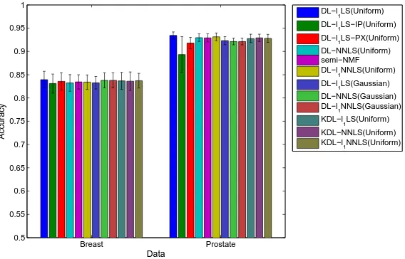
2.3 Accuracies of dictionary learning approaches. This is a color figure, thus the
readability may be affected if printed in grayscale. The order of the bars, from left to right, in the figure, is the same as these from top to bottom in
the legend. In the legend, the Gaussian and uniform priors are indicated
in the corresponding parentheses. IP and PX are the abbreviations of the interior-point and proximal methods, respectively. The rest dictionary
learn-ing models use active-set method without explicit notation. . . 45
2.4 Computing time of dictionary learning approaches. This is a color figure, thus the readability may be affected if printed in grayscale. The order of
the bars, from left to right, in the figure, is the same as these from top to
bottom in the legend. In the legend, the Gaussian and uniform priors are indicated in the corresponding parentheses. IP and PX are the abbreviations
of the interior-point and proximal methods, respectively. The rest dictionary learning models use active-set method without explicit notation. . . 46
2.5 The biological processes identified by our implementations of the standard
NMF (a) and VSMF (b), and by Ochset al.’s implementations of the standard
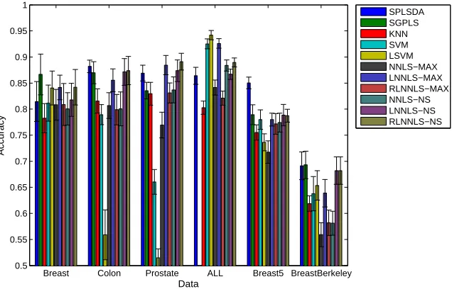
NMF (c) and CoGAPS (d) [1]. . . 56 2.6 Classification performance on six data sets. This is a color figure, thus the
readability may be affected if printed in grayscale. The order of the bars,
from left to right, in the figure, is the same as these from top to bottom in the legend. . . 66
2.7 Crucial difference diagram of the Nemenyi test (α= 0.05). . . 68 2.8 Computing time on six data sets. This is a color figure, thus the readability
may be affected if printed in grayscale. The order of the bars, from left to
right, in the figure, is the same as these from top to bottom in the legend. . 69
3.1 Heat map of NMF biclustering result. Left: the gene expression data where
each column corresponds to a sample. Center: the basis matrix. Right: the
coefficient matrix. This is a color figure, thus the readability may be affected if printed in grayscale. . . 84
3.2 Heat map of NMF clustering result on yeast metabolic cycle time-series data.
Left: the gene expression data where each column corresponds to a sample. Center: the basis matrix. Right: the coefficient matrix. This is a color figure,
thus the readability may be affected if printed in grayscale. . . 85
3.3 Biological processes discovered by NMF on yeast metabolic cycle time-series data. This is a color figure, thus the readability may be affected if printed in
grayscale. . . 86
3.4 Biological processes discovered by NMF on breast cancer time-series data. This is a color figure, thus the readability may be affected if printed in grayscale. 87
3.5 Mean accuracy and standard deviation results of NMF-based feature
extrac-tion on SRBCT data. This is a color figure, thus the readability may be affected if printed in grayscale. The order of the bars, from left to right, in
the figure, is the same as these from top to bottom in the legend. . . 89
3.6 The mean accuracy results of NNLS classifier for different amount of noise on SRBCT data. This is a color figure, thus the readability may be affected
if printed in grayscale. . . 91
3.7 The mean accuracy results of NNLS classifier for different missing value rates on SRBCT data. This is a color figure, thus the readability may be affected
3.8 The fitted learning curves of NNLS and SVM classifiers on SRBCT data. This
is a color figure, thus the readability may be affected if printed in grayscale. 92
3.9 Nemenyi test comparing 8 classifiers over 13 high dimensional biological data (α= 0.05). . . 93
4.1 A three-way tensor representation (left) and a heatmap representation (right)
of a GST data set. The black columns in the heatmap representation corre-spond to missing time points. . . 98
4.2 From Tucker3 decomposition (top) to Tucker1 decomposition (bottom). . . 102
4.3 Tensor factorization based feature extraction. . . 104
5.1 A schematic view which shows the difference between border patterns and
prototypes. . . 117
5.2 Plots of the synthetic data sets. This is a color figure, thus the readability
may be affected if printed in grayscale. . . 125
5.3 Performance on synthetic data. This is a color figure, thus the readability may be affected if printed in grayscale. The order of the bars, from left to
right, in the figure, is the same as these from top to bottom in the legend. . 127
5.4 The accuracies achieved on three-fold cross-Validation for the 17 real-life data sets. This is a color figure, thus the readability may be affected if printed in
grayscale. The order of the bars, from left to right, in the figure, is the same
as these from top to bottom in the legend. . . 130 5.5 An example of the hierarchical model. . . 132
6.1 (a) Unaligned profiles x(t) and y(t). (b) Aligned profilesx(t) and y(t), after applying y(t)←y(t)−amin. . . 141 6.2 (a) Yeast phases [2], (b) SCMA clusters , and (c) SCVV clusters for
Saccha-romyces cerevisiae. . . 150
6.3 (a) SCMA clusters and (b) SCVV clusters forSaccharomyces cerevisiae with
K = 10. . . 152 6.4 (a) SCMA clusters and (b) SCVV clusters with centroids shown, for
Schizosac-charomyces pombe. . . 153
7.1 An example of a Bayesian network representing a joint probability distribution.158
7.2 A Bayesian network, of which the BDeu and BIC scores are computed. . . . 165 7.3 An example of a second-order HO-DBN (top) and a non-stationary HO-DBN
7.4 An example of a DBN under the second-order stationary Markov assumption.
Left: stationary transition network. Right: the GRN obtained by folding the
transition network. . . 171 7.5 The true network and the predicted networks. . . 182
7.6 The gene regulatory network learned by MMHO-DBN. . . 183
7.7 The gene regulatory network learned by DBmcmc. . . 184 7.8 The gene regulatory network learned by DBN-ZC. . . 184
7.9 The true network from which simulated data are sampled. . . 191
7.10 The predicted networks using simulated data. . . 192 7.11 Effect of parameters on the performance of MMHO-DBN on the simulated
data. . . 193
7.12 The actualYeast5 networks and the predicted networks usingYeast5 data. 195 7.13 The actualYeast9 network and the predicted networks using Yeast9 data. . 196
7.14 Effect of parameters on the performance of MMHO-DBN when applied on
Yeast5on data. . . 198
7.15 Effect of parameters on the performance of MMHO-DBN when applied on
Yeast5off data. . . 199
7.16 Effect of parameters on the performance of MMHO-DBN when applied on
Yeast9 data. . . 199
8.1 Classification performance on SRBCT as missing rate increases. This is a color figure, thus the readability may be affected if printed in grayscale. . . 208
8.2 Graphical representation of Nemenyi test over microarray data with missing
rates 60% and 70%. . . 209 8.3 Tensor representation (a) and matrix representation (b) of a
gene-sample-time microarray data. . . 210
8.4 k-NN imputation with multiple-alignment. . . 212 8.5 Experimental procedure of imputation. . . 214
8.6 Errors of G*impute (a), S*impute (b), and GS*impute (c) methods, forg% = 0.1% to 20% andt= 1. . . 216 A.1 The mode-1 (a), mode-2 (b), and mode-3 (c) matricizations of the three-way
tensor shown in Figure 4.1. . . 222 A.2 PARAFAC decomposition. . . 224
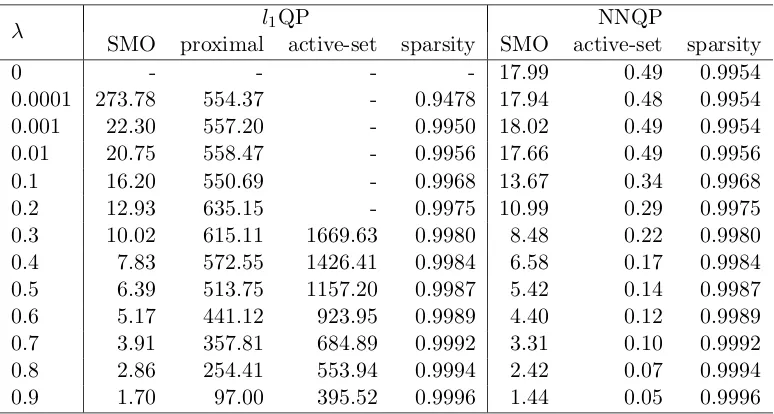
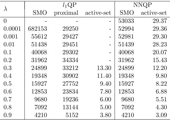
2.1 Mean computing time (in seconds) of each sample when using 5356 samples as training set. . . 37
2.2 Mean number of iterations of each sample when using 5356 samples as
train-ing set. . . 38 2.3 Mean prediction accuracies of the l1QP and NNQP models using 10-fold
cross-validation. . . 38
2.4 The existing NMF and SR models. . . 47 2.5 Classification performance of VSMF compared to the standard NMF. The
time is measure by stopwatch timer (theticandtocfunctions in MATLAB) in seconds. . . 54 2.6 The performance of MNNLS. . . 58
2.7 High dimensional microarray data sets. . . 65
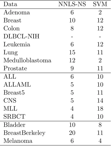
2.8 Minimum data size required to obtain significant accuracy (α= 0.05). NNLS-NS method only requires a very small number of training samples in order
to obtain significant accuracy. . . 70
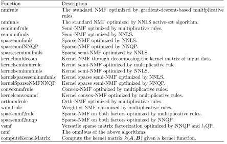
3.1 Algorithms of NMF variants. . . 77 3.2 NMF-based data mining approaches. . . 83
3.3 Gene set enrichment analysis using Onto-Express for the factor specific genes
identified by NMF. . . 85 3.4 Methods of sparse representation. . . 94
3.5 Sparse-representation based machine learning methods. . . 95
4.1 Classification performance of hidden Markov models on complete IFNβ data. 101 4.2 Classification performance of tensor factorization on complete IFNβ data. . 106 4.3 Comparison of running times on complete IFNβ data. . . 106 4.4 Comparison of classification performance of SVM on complete IFNβ data. . 109
4.5 Comparison of classification performance of sparse coding on complete IFNβ
data. . . 110
4.6 Comparison of classification performance of kernel dictionary learning on complete IFNβ data. . . 111 5.1 Summary of our NB methods and the benchmark methods used. . . 126
5.2 Results of the accuracies achieved by a three-fold cross-validation using the new and benchmark algorithms on the artificial data sets. . . 126
5.3 The real-life data sets used in our experiments. . . 128
5.4 Results of the accuracies achieved by a three-fold cross-validation using the new and benchmark algorithms on the real-life data sets. . . 129
5.5 The accuracy of the hierarchical model. . . 134 5.6 Current implementations of our RLMK toolbox. . . 135
6.1 Accuracies of SCMA and SCVV on two data sets. . . 153
7.1 Example data. . . 165 7.2 Frequency tables and (conditional) probability tables. . . 165
7.3 The comparison on simulated data. . . 181
7.4 The comparison of DBNs. . . 183 7.5 Current implementations of our probabilistic graphical models toolbox. . . . 189
7.6 Comparison on simulated data. . . 191
7.7 Comparison on real-life data. . . 197 7.8 Comparison of MMHO-DBN (first-order) and DBNmcmc on real-life data. . 197
7.9 Validating the time-delays on Yeast9. . . 198
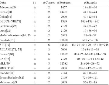
8.1 Microarray data sets. The sample size of each class and the total data size are in the last column. . . 208
8.2 Statistics for the five methods for 29 different percentages (from 0.1% to 20%) of genes which contain at most 1, 2, 3, 4, or 5 missing values, respectively.
There is no time point missing in this case. . . 215
8.3 Mean NRMS error for G*impute with at most one missing value for each selected time-series and one missing time point. . . 217
8.4 Mean NRMS error for S*impute with at most one missing value for each
selected time-series and one missing time point. . . 218 8.5 Mean NRMS error for GS*impute with at most one missing value for each
ν-NBN:ν-nearest border with normalized distance, 124
k-NN:k-nearest neighbors, 59, 115
l1LS:l1-least squares, 14
l1NNLS: l1-norm regularized non-negative least squares, 16 1-NN: 1-nearest neighbor, 90
3KNNimpute: three-wayk-nearest neighbor imputation, 211 3MAimpute: three-way multiple alignment imputation, 211
ALS: alternating least squares, 224
ANLS: alternating non-negative least squares, 224
ARLSimpute: autoregressive model based imputation, 204
BD: Bayesian decomposition, 75
BDe: Bayesian Dirichlet equivalence, 160
BDeu: Bayesian Dirichlet equivalence uniform, 162 BFRM: Bayesian factor regression model, 12
BI: border identification, 116
BIC: Bayesian information criterion, 160, 164 BN: Bayesian network, 157
BPCAimpute: Bayesian principal component analysis based imputation, 204
CANDECOMP: canonical decomposition, 223
CD: crucial difference, 67, 93
CMOS: classification by moments of order statistics, 118 CNN: condensed nearest neighbor, 116
CoGAPS: coordinated gene activity in pattern sets, 55, 75
CPD: conditional probability distribution, 158 CPT: conditional probability table, 158
DAG: directed acyclic graph, 157
DBmcmc: dynamic Bayesian network learning algorithm based on Markov chain Monte
Carlo, 181
DBN-ZC: Zou and Conzen’s dynamic Bayesian netowrk learning algorithm, 176
DBN: dynamic Bayesian network, 157
DiscHMMs: discriminative hidden Markov models, 100 DMMP: dynamic max-min parent, 177
ELM: extreme learning machine, 207
EM: expectation maximization, 82, 137, 159, 204
ENN: edited nearest neighbor, 116 ESS: equivalent sample size, 162, 180
FA: factor analysis, 9
FO-DBN: first-order dynamic Bayesian network, 157
GAimpute: gene-average imputation, 209
GenHMMs: generative hidden Markov models, 100
GIST: Gastrointestinal stromal tumor, 55
GKNNimpute: genek-nearest neighbor imputation, 210 GRN: gene regulatory network, 156
GSAimpute: gene-sample-average imputation, 209
GSEA: gene set enrichment analysis, 84
GSKNNimpute: gene-sample k-nearest neighbor imputation, 210
GSSVDimpute: gene-sample singular value decomposition imputation, 212
GST: gene-sample-time, 97, 202
GSVDimpute: gene singular value decomposition imputation, 212
HDI: highest density interval, 123
HDR: highest density region, 123
HK: hierarchical, 134
HO-DBN: high-order dynamic Bayesian network, 157
HONMF: high-order non-negative matrix factorization, 103, 225
HOOI: high-order orthogonal iterations, 104 HOOI: higher-order orthogonal iterations, 225
HOSVD: high-order singular value decomposition, 104, 225
IFNβ: interferon beta, 99
INDAFAC: incomplete data PARAFAC, 205
IRMA:in vivo reverse-engineering and modeling assessment, 194
KKT: Karush-Kuhn-Tucker, 21, 232
KNNimpute: k-nearest neighbor imputation, 90 KNNimpute: k-nearest-neighbor imputation, 203
KW-KPCA: kernel principal component analysis-based kernel whitening, 119
LASSO: least absolute shrinkage and selection operator, 14 LDR: linear dimension reduction, 101
LLSimpute: local least squares based imputation, 204
LNNLS: local non-negative least squares, 62 LRC: linear regression classification, 95, 207
LSVM: local support vector machine, 59
LTI: linear time invariant, 107
MA: multiple (time-series) alignment, 211
MAP: maximum a posteriori, 14
MCMC: Markov chain Monte Carlo, 12, 76, 167, 176 MDL: maximum description length, 176
ML: maximum likelihood, 163
MLDR: multilinear dimension reduction, 101 MLE: mixtures of local experts, 61
MMHC-BN: max-min hill-climbing Bayesian network, 168
MMHC: max-min hill-climbing, 157, 177
MMHO-DBN: max-min high-order dynamic Bayesian network, 157, 168
MMPC: max-min parent and children, 177
MNNLS: meta-sample based non-negative least squares, 57 mRMR: minimum redundancy maximum relevance, 262
MS: multiple sclerosis, 99
MSRC: meta-sample based sparse representation classification, 55, 207
NB-HP: nearest border approach based on hyperplane, 124
NB-HS: nearest border approach based on hypersphere, 124 NB: nearest border, 114
NMF: non-negative matrix factorization, 10
NN: nearest neighbor, 16, 115
NNLS: non-negative least squares, 15
NNQP: non-negative quadratic programming, 18, 79
NRMS: normalized root mean squared, 213
NS-NMF: non-smooth non-negative matrix factorization, 74 NS: nearest subspace, 16
NSPCA: non-negative sparse principal component analysis, 82
OBS: optimal brain surgery, 75
ODE: ordinary differential equation, 156
ortho-NMF: orthogonal non-negative matrix factorization, 81 OS: order statistics, 118
OVA: one-versus-all, 134
PARAFAC-ALS-SI: PARAFAC-alternating least squares with single imputation, 205 PARAFAC: parallel factors, 223
PC: parents and children, 167
PCA: principal component analysis, 9, 88 PGM: probabilistic graphical model, 157
PIN: protein interaction network, 176
PNN: prototypes for nearest neighbor, 116 PR: pattern recognition, 114
PRS: prototype reduction scheme, 116
PSVM: profile support vector machine, 60, 62
QP: quadratic programming, 17, 232
QPN: qualitative probabilistic network, 157, 184
RBF: radial basis function, 33
RLMK: regularized linear models and kernels, 134
RLNNLS: repetitive local non-negative least squares, 64 RNN: reduced nearest neighbor, 116
SAimpute: sample-average imputation, 209
SC: sparse candidate, 167
SCVV: spectral clustering with variation-based tranformation, 147
SGPLS: sparse generalized partial least squares, 65
SKNNimpute: sample k-nearest neighbor imputation, 210 SMO: self-organizing map, 137
SMO: sequential minimal optimization, 27, 264
SPLSDA: sparse partial least squares discriminant analysis, 65 SR: sparse representation, 9, 13
SRM: structural risk minimization, 229
SSVDimpute: sample singular value decomposition imputation, 212 STD: standard deviation, 53
SV: support vector, 238
SVDD: support vector domain description, 119, 255
SVDimpute: singular value decomposition based imputation, 204
SVM-RFE: support vector machine recursive feature elimination, 113, 262
SVM: support vector machine, 9, 113, 229 SVR: support vector regression, 242
TMG: text to matrix generator, 75
VC-dimension: Vapnik-Chervonenkis-dimension, 229
VCD: variation-based coexpression detection, 138, 144
VO-DBN: variable-order DBN, 176 VQ: vector quantization, 116
VSMF: versatile sparse matrix factorization, 45, 80
Introduction
1
Bioinformatics Challenges
In the area of biological and clinical study, a huge amount of various data, such as
genome-wide microarray gene expression data, proteomic mass spectrometry data, array compara-tive genomic hybridization data, and single nucleotide polymorphisms data, have been being
produced. These data provide us systemic information which allows us to conduct
genome-wide study, and therefore to reach more precise decisions and conclusions than ever before. Statistical learning and computational intelligence are among the main tools to analyze
these data. However, there are many difficulties that preventing an efficient and accurate
analysis. For example, there are usually tens of thousands of dimensions in microarray gene expression data, while its sample size is usually very small. With this problem, it may be
impossible to estimate the parameters of a model, as the number of sufficient samples needed increases exponentially as the number of dimensions. Second, the high-dimensional data
often have many redundant features when only few (maybe hidden) features correspond to
the desired study. This might drown useful information. In addition to the small sample size, the noise present in biological data and uncertainty in the target variable often lead to
overfitting of some models sensitive to noise and uncertainty. Furthermore, the structural
information in the data (for example the temporal information in time-series data) should be carefully taken into account in order to obtain better performance.
With the recent advances in microarray technology, the expression levels of genes with
respect to samples can be monitored synchronically over a series of time points. Such microarray data have three types of variables, genes, samples, and time points. Thus, they
can be represented by a three-way array data and are termed gene-sample-time (GST)
microarray data or GST data for short. The dimensionality of such data is much larger
than the two-way array data introduced above. Analyzing GST data can help discover the
pathway of many diseases due to genetic disorder, for example multiple sclerosis. Machine
learning and data mining approaches are among the main tools to analyzing GST data. First of all, since many existing machine learning methods are derived for two-way data
where each sample is represented by a vector, it is very challenging to cluster or classify
the three-way GST data where each sample is represented by a matrix. Second, the GST data may suffer from a much more severe issue of missing values, as the values of an entire
time point can be missing in a matrix sample. Many missing value imputation methods for
two-way data can not be directly applied on GST data.
Reconstructing gene regulatory networks (GRNs) is the key to understanding the
re-lations and pathways among thousands of genes and regulatory elements. One effort to
reach it is using high-throughput microarray gene time-series data. The rationality is based on the fact that the expression level of the genes at the current time can casually affect
the expression level of the genes in the subsequent time. There are many challenges in
reconstructing GRNs by learning a machine learning model on microarray gene time-series data. First, the expression levels of thousands of genes can only be sampled at a few time
points. If the number of the parameters of a model goes exponentially as the number of genes increases, we confront the curses of dimensionality. Second, the data are usually very
noisy, thus we should find a stochastic model to cope with it. Third, feedback regulation,
time-delayed interaction, and asynchronous regulation are the characteristics of the gene regulation events. A proper learning method should model all these features.
2
Sparse Machine Learning Models
The meaning of parsimony is twofold in machine learning: either the structure or (and) the parameter of a model can be sparse. Sparse models have many strengthes. First, sparsity
is an important regularization principle to reduce model complexity and therefore avoid
overfitting. Second, in many fields, for example bioinformatics, many high-dimensional data may be generated by a very few number of hidden factors, thus it is more reasonable
to use a proper sparse model than a dense model. Third, a sparse model is often easy to interpret. Therefore, in this dissertation, we investigate the sparse machine learning models
and their applications in high-dimensional biological data analysis. We focus our research
on five types of sparse models including sparse representation, sparse tensor factorization, sparse linear models, sparse spectral method, and sparse probabilistic graphical models.
by a sparse linear combination of basis vectors. From this point, we can also view the
well-known non-negative matrix factorization as a specific sparse representation model. Given a
new sample and basis vectors, learning the sparse coefficient is named sparse coding. Given the training data, learning the basis vectors is termed dictionary learning. Dictionary
learning is in essence the sparse matrix factorization. In the next chapter, we shall see
that, based on sparse representation, clustering, classification, and dimensionality reduction techniques can be devised for high-dimensional data.
Tensor factorization is the extension of matrix factorization in multi-way data which
is also called tensor. Basically matrix is a two-way tensor, and the GST data mentioned above can be represented as a three-way tensor. Therefore, sparse tensor factorization is
a suitable tool for analyzing GST data. In my thesis study, I investigate the high-order
non-negative factorization and other tensor decomposition models for the dimensionality reduction of GST data.
The parameter of the primal or dual form of the linear models (formulated as f(x) =
wTx+b) can be regularized to sparse. If the variable of a dual form is sparse, it implies that the model parameter w is a sparse linear combination of the training samples. The
training samples corresponding to non-zero coefficients are named support vectors. This can be applied as a sample selection technique for classification or regression. If the variable of
a primal form is sparse, that is the model parameterwis sparse, the target is approximated
as a sparse linear combination of features. The features corresponding to zero coefficients have no contribution, hence can be removed. This can serve as a feature selection technique
for high-dimensional data. In this thesis, I discuss many linear models using different
regularization terms and loss functions. Especially, I investigate novel techniques that extend linear models to multi-class data.
The spectral clustering method is a model that takes the similarity matrix as input,
and then solves the eigen-decomposition of the graph Laplacian matrix. If the weighted adjacency matrix (calculated based on the similarity matrix) is sparse, then the graph
Laplacian matrix is sparse as well. It has been shown that spectral clustering is very
efficient, because it is much more efficient to eigen-decompose a sparse matrix than a dense matrix. In my thesis study, I apply the spectral method to cluster microarray time-series
data. The alignment-based and variation-based transformations are used to compute the
similarity matrix.
In a graphical model with discrete variables, the number of parameters of a local
condi-tional distribution, corresponding to a node with its parents, increases exponentially as the
number of time points. Therefore, we have to limit the number of parents for each node
in order to learn the model parameters, which results in sparse structures. In my thesis
study, I investigate the high-order dynamic Bayesian networks to learn the gene regulatory networks from gene expression time-series data.
3
My Contributions
1. In Chapter 2, we explore sparse representation models for the classification and
di-mensionality reduction of various high-dimensional biological data. Our contributions
in this chapter include:
(a) We discuss the sparse representation from a Bayesian viewpoint.
(b) We propose the non-negative least squares based sparse coding model and inves-tigate their classification performance.
(c) We propose the weightedK-nearest neighbor rule for predicting class labels based on the sparse coefficient obtained by a sparse coding model.
(d) We propose kernel sparse coding models.
(e) We propose efficient active-set and decomposition methods for learning the pa-rameter of the sparse coding model.
(f) We propose two unified frameworks for dictionary learning. Under these
frame-works, we can easily extend the linear dictionary learning models to kernel ones.
(g) We investigate kernel-dictionary-learning based dimensionality reduction method
for high-dimensional biological data.
(h) We propose a supervised dictionary learning model for multi-class data based on sub-dictionary learning.
(i) We propose a cluster-and-classification approach, which is a local learning method, for classifying complexly distributed data.
2. In Chapter 3, we describe our implementations of the sparse representation models derived in Chapter 2 – non-negative matrix factorization toolbox (NMF toolbox) and
sparse representation toolbox (SR toolbox). The following are our contributions:
(a) The NMF algorithms, in our NMF toolbox, are relatively complete and
(b) Our NMF toolbox includes many functionalities for mining biological data, such
as clustering, biclustering, feature extraction, feature selection, and classification.
(c) The NMF toolbox also provides additional functions for biological data visual-ization, such as heat-maps and other visualization tools. They are pretty helpful
for interpreting some results. Statistical methods are also included for comparing
the performances of multiple methods.
(d) The SR toolbox include all the sparse coding and dictionary learning algorithms
mentioned Chapter 2.
(e) Based on the basic level of the SR algorithms, machine learning methods, in-cluding classification and dimensionality reduction, are implemented in our SR
toolbox.
3. In Chapter 4, we propose sparse tensor decomposition methods and kernel methods
for the dimensionality reduction and classification of gene-sample-time data. Our contributions are the following:
(a) We propose to apply the sparse tensor decomposition method, higher-order
non-negative matrix factorization, to reduce the dimensionality of the
gene-sample-time data efficiently.
(b) We apply kernel sparse coding and kernel dictionary learning methods for
clas-sifying matrix samples and extract vectorial features, respectively.
4. In Chapter 5, we propose two novel strategies to extend linear models to multi-class
data. The first one is an independent modeling, called nearest border method. The second one is a hierarchical model. Our contributions include:
(a) We propose the novel nearest border paradigm for multi-class classification
prob-lems, and implemented it by using a one-class SVM. This philosophy has not been
presented before in the literature.
(b) We propose the hierarchical model for multi-class classification problems. This
model is so flexible that any feature selection and classification methods can be
embedded in the model. We apply this model for gene selection and prediction of breast tumor subtypes, simultaneously.
(c) We realize most of the regularized linear models based methods mentioned in
Additionally, we conduct a thorough review on regularized linear models in Appendix
B where our contributions include:
(a) We review the main regularized (sparse) linear models using matrix notations,
unlike element-wise notations in most of the existing reviews. The formulations using matrices and vectors are succinct and easy to understand.
(b) Two main feature selection techniques based on SVM are also reviewed in details.
These techniques have been applied to gene selection in bioinformatics.
(c) We review the decomposition methods for two-class SVMs, and derive
decompo-sition methods for one-class SVMs.
5. In Chapter 6, we propose to use spectral method to cluster microarray time-series
data. We compare the alignment-based and validation-based transformations which are used to measure the similarities between pairs of time-series. The contributions
of this chapter are three-fold:
(a) We apply spectral clustering algorithms to expression time-series analysis.
(b) We propose new measurements for the quality of the spectral clustering approach.
(c) we empirically show that when applied to two well-known data sets, the
alignment-based transformation yields better clustering results than the variation-alignment-based
transformation.
6. In Chapter 7, we apply probabilistic graphical models on microarray gene expression time-series data to reconstruct the gene regulatory networks. We have the following
contributions:
(a) We propose themax-min high-order dynamic Bayesian network (MMHO-DBN)
learning algorithm, in order to reconstruct time-delayed gene regulatory
net-works.
(b) We apply the qualitative probabilistic networks (QPNs), after obtaining a DBN,
to interpret the interactions learned using the concepts of influence and synergy.
(c) We have implemented the MMHO-DBN and QPNs in MATLAB, and published
it online.
7. In Chapter 8, we explore various strategies for learning models from incomplete
(a) We extend the existing imputation methods, originally for two-way data, to
methods for gene-sample-time data.
Sparse Representation for
High-Dimensional Data Analysis
1
Introduction
1The studies in biology and medicine have been revolutionarily changed since the inventions
of many high-throughput sensory techniques. Using these techniques, the molecular
phe-nomena can be probed with a high resolution. In the virtue of such techniques, we are able to conduct systematic genome-wide analysis. In the last decade, many important results have
been achieved by analyzing the high-throughput data, such as microarray gene expression
profiles, gene copy numbers profiles, proteomic mass spectrometry data, next-generation sequences, and so on.
On one hand, biologists are enjoying the richness of their data; one another hand,
bioinformaticians are being challenged by the issues of high-dimensional data as well as by the complexity of bio-molecular data. Many of the analysis can be formulated as machine
learning tasks. First of all, we have to face the cures of high dimensionality, which means
that many machine learning models are unable to correctly predict the classes of unknown samples due to the large number of features and the small number of samples in such
data. In other words, the machine learning models can be overfitted and therefore have poor capability of generalization. Second, if the learning of a model is sensitive to the
dimensionality, the learning procedure could be extremely slow. Third, many of the data
are very noisy, therefore the robustness of a model is necessary. Fourth, the high-throughput data exhibit a large variability and redundancy, which make the mining of useful knowledge
1
This section is based on our publication [3].
difficult. Moreover, the observed data usually do not tell us the key points of the story. We
need to discover and interpret the latent factors which drive the observed data.
Many of such analyses are classification problems from the machine learning view-point. Therefore in this study, we focus our study on the classification techniques for
high-dimensional biological data. The machine learning techniques addressing the
chal-lenges above can be categorized into two classes. The first one aims to directly classify the high-dimensional data while keeping a good generalization ability and efficiency in
op-timization. The most popular method in this class is the regularized basis-expanded linear
model. The regularization aims to avoid overfitting a model by reducing the model
com-plexity while fitting it. One example is the state-of-the-artsupport vector machine (SVM)
[4]. SVM is sparse linear model that uses hinge loss andl2-norm regularization. It can be kernelized and its result is theoretically sound. Combining different regularization terms and various loss functions, we can have many variants of such linear models [5]. In addition
to classification, some of the models can be applied to regression and feature (bio-marker)
identification. However, most of the learned linear models are not interpretable, while inter-pretability is usually the requirement of biological data analysis. Moreover, linear models
can not be extended naturally to multi-class data, while in bioinformatics a class may be composed of many subtypes. See Appendix B for a through discussion on linear models.
Another technique of tackling with the challenges above is dimensionality reduction
which includes feature extraction and feature selection. Principal component analysis (PCA) [6] is one of the traditional feature extraction methods and is widely used in
process-ing high-dimensional biological data. The basis vectors produced by PCA are orthogonal,
however many patterns in bioinformatics are not orthogonal at all. The classicfactor anal-ysis (FA) [7] also has orthogonal constraints on the basis vectors, however its Bayesian
treatment does not necessarily produce orthogonal basis vectors. Bayesian factor analysis
will be introduced in the next section.
Sparse representation (SR) [8] is a parsimonious principle that a sample can be
approx-imated by a sparse linear combination of basis vectors. Non-orthogonal basis vectors can
be learned by SR, and the basis vectors may be allowed to be redundant. SR highlights the parsimony in representation learning [9]. This simple principle has many strengthes
that encourage us to explore its usefulness in bioinformatics. First, it is very robust to
redundancy, because it only selects few among all of the basis vectors. Second, it is very robust to noise [10]. Furthermore, its basis vectors are non-orthogonal, and sometimes are
interpretable due to its sparseness [11]. There are two techniques in SR. First, given a basis
training data, learning the basis vector is calleddictionary learning. As dictionary learning
is, in essence, a sparse matrix factorization technique. Non-negative matrix factorization
(NMF) [12] can be viewed a specific case of SR. For understanding sparse representation better, we will give the formal mathematical formulation from a Bayesian perspective in
the next section.
Contributions: In this chapter, we investigate sparse representation for high-dimensional
data analysis comprehensively. We explore various sparse representation models for the
classification and dimensionality reduction of high-dimensional biological data. We propose kernel and supervised sparse representation models. Efficient optimization algorithms are
devised for them. Our contributions in this chapter include:
1. We discuss the sparse representation from a Bayesian viewpoint.
2. We propose the non-negative least squares based sparse coding model and investigate
their classification performance.
3. We propose the weightedK-nearest neighbor rule for predicting class labels based on the sparse coefficient obtained by a sparse coding model.
4. We propose kernel sparse coding models.
5. We propose efficient active-set and decomposition methods for learning the parameter
of the sparse coding model.
6. We propose two unified frameworks for dictionary learning. Under these frameworks, we can easily extend the linear dictionary learning models to kernel ones.
7. We investigate kernel-dictionary-learning based dimensionality reduction method for
high-dimensional biological data.
8. We propose a supervised dictionary learning model for multi-class data based on
sub-dictionary learning.
9. We propose a cluster-and-classification approach, which is a local learning method,
for classifying complexly distributed data.
The rest of this chapter is organized as follows. First, we formulate sparse representation from a Bayesian viewpoint in Section 2. Then, we discuss sparse-coding based
investigate dictionary learning based dimension reduction techniques in Section 6. In this
section, we present a generic dictionary learning framework which can be easily kernelized.
In Section 7, a more general model called versatile sparse matrix factorization is proposed. We then propose a supervised dictionary learning method for multi-class data in Section 8.
Finally in Section 9, we propose a novel local classification approach, called
clustering-and-classifying, that combines both dictionary learning and sparse coding.
2
Bayesian Sparse Representation
2Both (sparse) factor analysis and sparse representation models can be used as dimension reduction techniques. Due to their intuitive similarity, it is necessary to give their definitions
for comparison. In this section, we briefly survey the sparse factor analysis and sparse
representation in a Bayesian viewpoint. The introduction of sparse representation is helpful to understand the content of the subsequent sections. Hereafter, we use the following
notations unless otherwise stated. Suppose the training data is D ∈ Rm×n (m is the
number of features and n is the number of training instances (samples or observations)), the class information is in the n-dimensional vector c. Suppose p new instances are in
B ∈Rm×p.
2.1 Sparse Bayesian (Latent) Factor Analysis
The advantages ofBayesian (latent) factor analysis model[13] over likelihood (latent) factor analysis model are that
1. The knowledge regarding the model parameters from experts and previous
investiga-tions can be incorporated through the prior.
2. The values of parameters are refined using the current training observations.
The Bayesian factor analysis model [13] can be formulated as
(b|µ,A,x, k) =µ+Ax+, (2.1)
where b ∈ Rm×1 is an observed multivariate variable, µ ∈
Rm×1 is the population mean,
A∈Rm×k islatent factor loading matrix, andx∈
Rk×1islatent factor score (km), and
∈Rm×1 is an idiosyncratic error term. In Equation (2.1), we list the model parameters,
{µ,A,x, k}, explicitly on the righthand side of “—”. This model is restricted by the following constraints or assumptions:
1. The error term is normally distributed with mean0 and covarianceΦ: ∼N(0,Φ).
Φis usually diagonal.
2. The factor score vector is also normally distributed with mean 0 and identity covari-ance R = I: x ∼ N(0,R); and the factor loading vector is normally distributed:
ai ∼N(0,∆) where ∆ is diagonal. Alternatively, the factor loading vectors can be
normally distributed with mean0and identity covariance∆=I; and the factor score vector is normally distributed with mean0 and diagonal covariance R. The benefit
of identity covariance either on xorAis that arbitrary scale interchange between A
and xdue to scale invariance can be avoided.
3. xis independent of .
For ntraining instancesD, we have the likelihood:
p(D|µ,A,Y,Φ, k) = 1 (2π)mn2 |Φ|
n 2
e−12 Pn
i=1(di−µ−Ayi)TΦ−1(di−µ−Ayi)
= 1
(2π)mn2 |Φ| n 2
e−12trace[(D−µ1
T−AY)TΦ−1(D−µ1T−AY)]
, (2.2)
where trace(M) is the trace of square matrix M.
The variants of Bayesian factor analysis models differ in the decomposition of the joint
priors. The simplest one may be p(µ,A,Y) =p(µ)p(A)p(Y). Suppose k is fixed a priori. The posterior therefore becomes
p(µ,A,Y|D, k)∝p(D|µ,A,Y,Φ, k)p(µ)p(A)p(Y). (2.3) The model parameters are usually estimated via Markov chain Monte Carlo (MCMC)
techniques.
Sparse Bayesian factor analysis model imposes a sparsity-inducing distribution over
the factor loading matrix instead of Gaussian distribution. In [14], the following mixture of
prior is proposed:
p(aij) = (1−πij)δ0(aij) +πijN(aij|0,1), (2.4)

![Figure 2.5: The biological processes identified by our implementations of the standardNMF (a) and VSMF (b), and by Ochs et al.’s implementations of the standard NMF (c)and CoGAPS (d) [1].](https://thumb-us.123doks.com/thumbv2/123dok_us/1411362.1173731/88.612.122.526.118.495/figure-biological-processes-identied-implementations-standardnmf-implementations-standard.webp)