Performance and Analysis of Channel Estimation Techniques for LTE Downlink System under Fading with Mobility

Performance and Analysis of Channel

Estimation Techniques for LTE Downlink

System under Fading with Mobility

Khushboo A. Parmar1, Saurabh M. Patel2

ME Student, Dept. of E&C, Sardar Vallabhbhai Patel Institute of Technology, Vasad, Gujarat, India1

Asst. Professor, Dept. of E&C, Sardar Vallabhbhai Patel Institute of Technology, Vasad, Gujarat, India2

ABSTRACT: The Long term evolution (LTE) is the current extension of the third generation (3G) mobile

communication system that provides high improvement in data rate, coverage and spectral efficiency. Since downlink is always an important factor in coverage and capacity aspects, special attention has been given in selecting technologies for LTE downlink. In proposed work, least square error (LSE) and minimum mean square error (MMSE) channel estimation techniques are presented for long term evolution (LTE). The performance of two channel estimators for LTE Downlink systems, the Least Square Error (LSE) and the Minimum Mean Square Error (MMSE) are studied and finally compared their simulation results under different multipath fading. The proposed work will demonstrate the efficiency of LSE and MMSE over different Fading channel like AWGN, Rayleigh fading and Nakagami fading with mobility and without mobility. Then, a polynomial interpolation algorithm using the method of Lagrange is represented which greatly reduces the complexity of the transceiver. MATLAB simulations are used to evaluate the performance of the studied estimators. These simulation results show that Lagrange interpolation technique performs better than MMSE and LSE for both the case without mobility and with mobility under all three multipath fading channels. Further, mobility increases the Mean Square Error (MSE) of the system.

KEYWORDS: Long Term Evolution (LTE); Orthogonal Frequency Domain Multiple (OFDM); Multiple Input

Multiple Output (MIMO); Channel Estimation; Pilot Symbol; Least Square Error (LSE); Minimum Mean Square Error (MMSE); Mean Square Error (MSE); Signal-to-Noise Ratio (SNR);

I. INTRODUCTION

To satisfy an increasing demand for high data rate with available limited spectrum for wireless communication, 3rd Generation Partnership Project (3GPP) introduces Long Term Evolution (LTE). LTE provides high data-rate, low latency and flexible bandwidth [1]. Theoretically, LTE offers a speed of 100 and 50 Mbits/s in the Downlink and Uplink transmissions respectively with 20 MHz bandwidth [2],[3]. LTE Downlink systems take on Orthogonal Frequency Division Multiple (OFDM) and MIMO to provide up to 100 Mbps for 2x2 MIMO systems [3]. OFDM is used to combat the effect of frequency selective fading and can improve the spectral efficiency of the system [2],[3]. OFDM converts the frequency selective channel into parallel flat-fading sub-channels. Increase in the capability of channel and reduction of signal fading are achieved by MIMO system which sends particular information through multiple antennas simultaneously [3].

Bandwidth offered to wireless communication systems is limited by a series of factors, the most important of which is the nature of the wireless channel. A significant characteristic of the wireless channel is multipath fading, which consists in the variation of the channel strength over time and frequency, due to constructive and destructive superposition of multiple paths travelling from the transmitter to the receiver through the wireless medium.

systems occurs if the estimation at the receiving end is not correct. Multiple channel estimation algorithms can be employed for estimation purpose.

This project is aimed to perform Least Square estimation (LSE) and Minimum Mean Square estimation (MMSE) for different fading channel which include AWGN, Rayleigh fading and Nakagami fading Channel. Finally we will demonstrate the efficiency of our LSE and MMSE over different Fading channels with mobility and without mobility. Further, to make the estimation more efficient, a polynomial interpolation algorithm will be presented using the Lagrange method.

This paper organized as follows. Section II contains related work of channel estimation on LTE Downlink system, section III provides the system model and the channel estimation techniques of LTE downlink systems, section IV describes of LTE under multipath fading and then section V explains the Lagrange polynomial interpolation algorithm for channel estimation of LTE. Finally, the results and the conclusion are specified in section VI and section VII respectively.

II. RELATED WORK

In [1] four channel estimation algorithms for the MIMO LTE downlink systems have been compared. For uncoded systems, the simulation results show that the LS estimation combined with Linear interpolation affords very good performances and moderate complexity as well as strength to channel conditions. Linear and Spline interpolations are lower complex than LS and perform worst. Lattice interpolation is not suitable for the LTE downlink systems because of the reference signals grid design. For the coded system, the same trends are experienced but the performance improves appreciably.

In [2] channel estimation for LTE downlink based on the interpolation to estimate channel coefficients. Lagrange polynomial interpolation method is proposed. Here, they perform the estimation for downlink LTE system for Single-Input Single- Output (SISO) and MIMO transmission then compare the obtained results with linear and Sinus Cardinal Interpolations. The simulation results show that the Lagrange method outperforms the linear interpolation in term of Block Error Rate (BLER) and throughput vs. Signal to Noise Ratio (SNR). Despite the complexity of this algorithm, it offers significant improvement of the performance of LTE downlink system.

In [3] the performance of two linear channel estimators for LTE Downlink systems, the Least Square Error (LSE) and the Linear Minimum Mean Square Error (LMMSE) using QPSK and 16 QAM modulation techniques are studied and also studied the effect of channel length on the performance of channel estimation. Matlab simulations are used to evaluate the proposed work for 2 x 2 LTE downlink system. Simulation of results for length of CP greater or equal to channel length indicate superior performance of LMMSE compared to LS estimator at the cost of the increased complexity since it depends on statistics of channel and noise . In the other case, LMMSE provides better performance only for low SNR values and begins to lose its performance for higher SNR values. Whereas, LS gives superior performance than LMMSE in this range of SNR values.

In [4] an optimum pilot pattern design can improve the spectral efficiency and reliability of an OFDM system. In this paper the problem of pilot pattern design is solved for SISO-OFDM system. In this work, the same average power in pilot symbols and the data symbols are kept maintained but the distance between the pilots varies. The new pilot design gives the best performance in terms of BER is established as the optimum pilot pattern. Equi-powered and equi-spaced pilot-symbols gives the lowest MSE and maximum channel capacity.

In [9] hardware implementation aspects of the channel estimator in 3GPP LTE terminals are investigated. In this, the channel estimator presented boosts the throughput at feasible silicon by adopting estimation method named Approximate Linear Minimum Mean Square Error (ALMMSE). Simulation results shows that the LMMSE channel estimator outperforms the LS and ALMMSE estimators. However, its hardware implementation requires the most computational power. It supports 20MHz downlink bandwidth.

III. LTEDOWNLINK SYSTEM

A. System model of LTE Downlink :

system and provides strength to the transmitted signal against the multipath effect. By transmitting the same information simultaneously through multiple antennas, channel capability is increased by MIMO system along with reduced signal fading. Without increasing resources for base bands and power output, LTE system combines these two powerful technologies (MIMO-OFDM) to delivers superior spectral efficiency and successful message delivery rate [2].

X(k) x(n) xf(n)

Y(k) y(n) yf(n)

Output Data

W(n)

Fig.1 Baseband OFDM System [5]

Figure 1 shows basic block diagram of OFDM transceiver architecture. Suppose the serial data X is first converted into the parallel streams x1,x2,x3,...,xk. Then pilots are inserted either to all sub-carriers with a specific period or uniformly

between the information data sequence. After that the Inverse Fast Fourier Transform (IFFT) is performed on parallel data stream. IFFT transforms the data sequence of length N{X(k)} into time-domain signal {x(n)}. Then the parallel data stream is converted back to the serial data and guard interval is inserted. Between consecutive OFDM symbols, a guard interval is inserted to avoid the Inter Symbol Interference (ISI). Then the ISI can be eliminated almost entirely, but a rapid change of waveform contains higher spectral components, so they produce Inter Carrier Interference (ICI). So a guard interval with cyclic prefix is used to avoid the Inter Carrier Interference (ICI). A copy of the last part of the OFDM symbol is attached to its front is called a Cyclic Prefix (CP). The transmitted signal xf(n) will pass through the

frequency selective time varying fading channel with additive noise. The received signal is given by [5]:

yf(n) = xf(n) O h(n) + w(n) (1)

Where, w(n) is additive white Gaussian noise and h(n) is channel impulse response.

At the receiver, guard time is removed after passing to discrete domain through LPF. Then y(n) is sent to FFT block to recover the time domain signal [5].

Y(k) = X(k)H(k) + I(k) + W(k) k=0,1,...N-1 (2) After FFT block, pilot signals are extracted and estimated channel He(k) for the data sub-channels is obtained in

channel estimation block. Then the transmitted data is estimated by [5]: Xe =

( )

( ) k=0,1,2,...,N-1 (3)

Then the binary information data is obtained back in “signal demapper” block.

MIMO multiplies capacity by transmitting different signals over multiple antennas, and, OFDM divides a radio channel into a large number of closely spaced sub-channels to provide more reliable communications at high speeds. Consider 2X2 MIMO system (2 Transmitter & 2 Receiver) which is shown in figure 2.

Pilot

Insertion _IFFT Guard

Insertion P/S

Map S/P

S/P Guard

Removal FFT

Channel Estimation P/S

Demap

Channel

Fig. 2 2X2 MIMO system

Here two transmitter antennas (TX#1 and TX#2) and two receiver antennas (RX#1 and RX#2) are used. The received signal on first receiver antenna (RX#1) is

= ℎ +ℎ + (4) The received signal on second receiver antenna (RX#2) is

= ℎ +ℎ + (5) The matrix representation of the received signal is

= ℎ ℎ

ℎ ℎ + (6)

During OFDM signal production, cyclic prefix (CP) insertion is an essential function. In order to prevent interference from OFDM symbols which are earlier transmitted, it is required to have cyclic prefix. The CP represents redundant information and an important overhead. The name “prefix” implies discarding the first portion of the received OFDM signal at the receiver. Hence it is necessary for LTE to specify smallest possible CP to get maximum spectral efficiency with a minimum overhead.

Table 1. Normal and extended cyclic prefix specifications [14]

Configuration Subcarrier spacing (Δf)

(kHz)

No. Of sub-carrier per resource block

No. Of OFDM symbols per resource

block

Normal cyclic prefix 15 12 7

Extended cyclic prefix 15 12 6

Table 1 depicts LTE standard having two CP values for subcarrier spacing of 15 kHz i.e. normal (4.7 μs) and

extended (16.6 μs). For transmissions over most urban and suburban environments normal CP length is appropriate

which reflects typical delay spread values for those environments. The extended CP length is associated with excess overhead and is required for rural areas which need long delay spreads and for broadcasting services [14].

Fig.3 LTE time-domain structure [14] _{Fig.4Resource elements, blocks, and grid}[14]

Figure 3 shows the time-domain structure of the LTE. It assembles the transmission as a sequence of 10 ms length radio frames which are further divided into 10 subframes of 1 ms lengths. A typical subframe contains two 0.5 ms slot lengths. Each slot contains seven or six OFDM symbols considering usage of a normal or an extended CP [14].

Resource grid is a plot of time (x-axis) and frequency (y-axis). Time wise OFDM symbol of a resource element is indicated by x-coordinate whereas the frequency wise OFDM subcarrier is indicated by y-coordinate [14]. It is also called time-frequency representation of signal. Figure 4 shows the LTE downlink resource grid containing normal CP. A resource element is indicated at the meeting point of an OFDM symbol with a subcarrier of 15 kHz spacing. Normal CP contains 7 symbols for each slot or 14 OFDM symbols for each subframe. Resource elements are grouped in the frequency domain pertaining to 12 subcarriers i.e. 180 kHz (12 subcarriers x 15kHz spacing) and in the time domain with one 0.5ms slot. Such group is defined as a Resource block. Each resource block contains 84 resource elements (12 subcarriers x 7 OFDM symbols) for a normal CP with 7 OFDM symbols for each slot. On the other hand, the resource block contains 72 resource elements (12 subcarriers x 6 OFDM symbols) for extended CP with six OFDM symbols for each slot. In terms of frequency-domain arrangement, the resource block (RB) is an important unit of LTE frame structure as it is a representation of the smallest unit of transmission [14].

In LTE standard pilot symbols are inserted at specific position in each PRB. Pilot symbols are also referred as reference signals. These pilots transmitted from multiple antennas are orthogonal to each other [5]. The null sub-carriers are represented by black crosses in order to protect interference of the reference signals of a particular antenna with data and pilots of remaining antennas [5].

B. Channel Estimation Techniques for LTE Downlink System:

In pilot-based channel estimation of LTE downlink, performance of below two estimators are efficient. 1. Least Square Error (LSE) Channel estimator

2. Minimum Min Square Error (MMSE) Channel estimator.

1. LSE channel estimator:

The Least Square (LS) channel estimator for subcarriers on which pilot symbols are located, is given by[5],

ℎ = yp (7)

ℎ ℎ = LS estimation channel frequency response = transmitted symbols

The LS estimate of such system is obtained by minimizing the square distance between the received signal and the original signal. This estimation procedure is simple and easy to implement. But it has high mean square error (MSE). The error is given by the difference between expected output Y′ and the received symbol Y [10],

E = Y′ – Y (8) The MSE is defined as [10],

MSE = E [(Y′ – Y)2] (9) The MSE should be reduced in order to recover the original transmitted symbol at receiver [10].

2.MMSE channel estimator:

The MMSE channel estimation employs the channel statistics to minimize the MSE estimate of the channel responses given by [3],

= RHHp (RHpHp + (XXH)-1) ℎ (10)

Where, RHHp = Cross correlation matrix between all subcarriers and the subcarriers with reference signals

RHpHp = Autocorrelation matrix of the subcarriers with reference signals

Due to the inversion matrix lemma, the complexity of MMSE estimator is high. Every time inversion is needed, data changes. By averaging the transmitted data, the complexity of this estimator can be reduced. Therefore we replace the term,

(XXH)-1 = E[(XXH)-1] Therefore the simplified MMSE estimator becomes,

= RHHp (RHpHp+(β/SNR)Ip)-1 ℎ (11)

Where, β is scaling factor depending upon the constellation value of 1 for QPSK and 17/9 for 16 QAM.

IV. LTEUNDER MULTIPATH FADING

Fading is rapid fluctuations of the amplitudes, phases or multipath delays of a signal over a short period of time or travel distance. Fading is caused by interference between two or more transmitted signals which arrive at the receiver at slightly different times [13].

For mobile communication, multipath propagation causing selective frequency channels may causes serious problems. Therefore, Multicarrier modulation (MC), especially Orthogonal Frequency Division Multiplexing (OFDM) which is used to conflict the effect of frequency selective fading. OFDM consists of converting a frequency-selective fading channel into parallel flat-fading sub-channels [12].

Frequency selective fading is due to time dispersion of the transmitted symbols within the channel. Thus the channel includes intersymbol interference (ISI). Frequency selective fading channels are much more complicated to model, since each multipath signal must be modelled and the channel must be considered to be linear filter [13]. When analyzing mobile communication systems, statistical impulse response models such as Gaussian model, Rayleigh fading and Nakagami fading model are generally used for analyzing frequency selective small scale fading.

1. Gaussian Distribution (AWGN Channel):

The Gaussian distribution has a probability density function (pdf) given by [13]

p (r) =

√ exp( -

( )

) (12)

where, r is a random variable with mean μ and variance σ.

2. Rayleigh Distribution:

When during the signal propagation in wireless communication, there is no (Line Of Sight) LOS component between mobile and BS, received signal consist of reflection and scattering wave from different directions and follow Rayleigh distribution[13].

The Rayleigh distribution has a probability density function (pdf) given by

p (r) = exp( - ) ;(0<=r<=∞)

In this paper, channel estimation is performed for LTE downlink under these two- Gaussian and Rayleigh fading. Their simulation results for both the channel estimation techniques- LSE and MMSE- are compared for 16 QAM and 64 QAM techniques.

3. Nakagami Fading Channel:

Rayleigh fading falls brief in describing long-distance fading outcomes with sufficient accuracy. This truth changed into first determined by way of Nakagami, who then formulated a parametric gamma distribution-primarily based density characteristic, to explain the experimental data he acquired. It become then showed by way of many researchers the use of actual-life information that the model proposed via Nakagami gives a better clarification to much less and more extreme situations than the Rayleigh and Ricean version and affords a better in shape to the mobile communication channel information [11].

Nakagami distribution does not assume a LOS conditions, but use a parametric gamma distribution-based density function. The PDF of Nakagami distribution is [11]

( ) =2

Ω Γ(m) exp

−

≥1

2, ≥0 (14) Where, = average power of multipath scatter scattered field

Γ(m) = the gamma function

At the physical layer, channel characteristics vary with the location of the user and because of mobility, vary in time. The Doppler shift defines the coherence time, which is the duration of time. The separation of the pilot tones in the LTE is 0.5ms. Pilot tones or reference signals are used to sample the channel to perform equalization and other tricks. The Doppler shift defines the maximum sampling period that will allow to sample the channel correctly. If the channel can change as fast as every 0.5ms, one needs to have one sample at least ever 0.5ms. Therefore, the reference signals are separated every 0.5ms.

V. LAGRANGE POLYNOMIAL INTERPOLATION

Fig.5 Flow chart of Lagrange Polynomial Interpolation algorithm[2]

The Lagrange polynomial is given by the following expression,

( ) = ( ) (15) Initialization

Extract Pilots

LS ( )

Put ( ) in

(i,k)

≠

(i,k)(P

Rank of Poly n

Calculate L0……..Ln

Calculate N0...Nn-1

= Poly(n)

BLER optimum

= ( )

Index of

( )

(i.k)++

Yes

No

n++

Yes _No

( )

( ) = −

− (16)

Where yi = pilots

L = coefficient of Lagrange n = Lagrange polynomial order

For MIMO system model, the received signal consisting of NTtransmits antennas and NR receives antennas can be represented by the following Equation:

( ) ( )

= _{( )}( ) _{( )}( )+ (17) Where ( )

( )

= [ ⋯ ⋯ ] is the received vector _{( )}( ) = Channel coefficient matrix of the dimensions NTxNR

N = [n1, n2, ...nNR ] is the noise vector

Here, for temporary, the Lagrange polynomial interpolation is used for frequency domain and linear interpolation. The steps for interpolation algorithm are represented as follow:

1. Extract ( ) pilots from received signal .

2. Calculate channel coefficients of pilots symbols with LS estimator

( )=

( )

( )

(a)

3. Calculate L0,……..,Ln coefficients of Lagrange with n order of Lagrange Polynomial and p index of pilots. For

n=2 and in order to estimate first 12 coefficients we use 3 pilots to be placed at xp0 = 0, xp1 = 6 and xp2 = 12.

L0 = ((xi-xp1)*(xi-xp2)) / (xp0-xp1)*(xp0-xp2)) (b)

L1 = ((xi-xp0)*(xi-xp2)) / (xp1-xp0)*(xp1-xp2)) (c)

L2 = ((xi-xp0)*(xi-xp1)) / (xp2-xp0)*(xp2-xp1)) (d)

where, xi is freq. index of to estimate

4. Estimate using Lagrange polynomial:

= L0 * ( ) + L1 * ( ) + L2 * ( ) (e)

where, ( ), ( ) and ( ) are three successive pilots.

5. Testing the operation performance by incrementing the polynomial of order n until having optimal performance.

VI. SIMULATION RESULTS

Table 2. Simulation Parameter

Parameter Value

Bandwidth 20MHz

No. Of subcarriers NSC 2048

Subcarrier spacing ∆ 15KHz

No. Of RB 10

Modulation scheme 16-QAM, 64-QAM

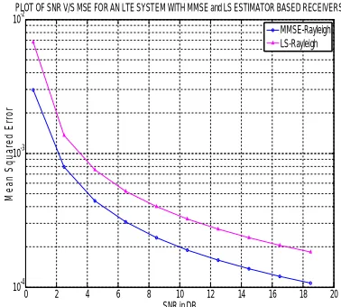
fig. 6 MSE vs SNR plot of LS and MMSE channel estimation for Fig.7 SNR vs MSE for an LTE with LS and MMSE estimators for

an LTE system with AWGN channel Rayleigh fading channel

Fig.6 shows that MMSE gives less MSE compared to LS, hence it is best technique. But it has higher computational complexity. Fig. 7 demonstrates the simulation results which show the comparison between LS and MMSE channel estimation for Rayleigh fading with zero mobility. The performance of LS and MMSE channel estimators are simulated in terms of Mean Square Error (MSE) and Signal-to-Noise Ratio (SNR) for Rayleigh fading. From fig.6, it is seen that MMSE gives approximately 3dB better performance than LS, but with computational complexity

.

Fig. 8 MSE Vs SNR plot of LS and MMSE for an LTE system Fig. 9 MSE Vs SNR plot of LS, MMSE and proposed Lagrange

for Nakagami fading channel interpolation techniques for an LTE system for Gaussian channel

From fig.8, it is seen that MMSE gives approximately 3dB better performance than LS, but with computational complexity. Figure 9 shows the simulation plot of MSE vs SNR of Lagrange polynomial interpolation technique and further its comparison with the previous estimation techniques-LS and MMSE. From the graph, it is seen that Lagrange interpolation is little bit better than MMSE, but computationally Lagrange is less complex compared to MMSE. So it can be concluded that Lagrange interpolation technique is better than LS and MMSE.

0 2 4 6 8 10 12 14 16 18 20

10-2

10-1

100

101

102

SNR in DB

M e a n S q u a re d E rr o r

PLOT OF SNR V/S MSE FOR AN LTE SYSTEM WITH MMSE and LS ESTIMATOR BASED RECEIVERS

MMSE LS

0 2 4 6 8 10 12 14 16 18 20

10-4

10-3

10-2

SNR in DB

M e a n S q u a re d E rr o r

PLOT OF SNR V/S MSE FOR AN LTE SYSTEM WITH MMSE and LS ESTIMATOR BASED RECEIVERS

MMSE-Rayleigh LS-Rayleigh

0 2 4 6 8 10 12 14 16 18 20

10-2

10-1

100

SNR in dB

M e a n S q u a re d E rr o r

PLOT OF MSE V/S SNR FOR AN LTE SYSTEM WITH NAKAGAMI FADING CHANNEL

LS-Nakagami MMSE-Nakagami

0 2 4 6 8 10 12 14 16 18 20

10-4 10-3 10-2 10-1 100

SNR in dB

M e a n S q u a re d E rr o r

PLOT OF MSE V/S SNR FOR AN LTE SYSTEM

Fig. 10 MSE Vs SNR plot of LS, MMSE and Lagrange interpolation Fig. 11 MSE Vs SNR comparison plot of LS, MMSE and Lagrange

techniques for an LTE system under Rayleigh fading interpolation techniques for an LTE system under Nakagami fading

Figure 10 shows the simulation plot of MSE vs SNR of Lagrange polynomial interpolation technique and further its comparison with the previous estimation techniques-LS and MMSE under the effect of Rayleigh fading. It is seen that Lagrange interpolation is little bit better than MMSE, but computationally Lagrange is less complex compared to MMSE. So it can be concluded that Lagrange interpolation technique is better than LS and MMSE. Figure 11 shows MSE plot of LS, MMSE and Lagrange interpolation technique under the effect of Nakagami fading channel for LTE system. Here, Lagrange interpolation technique gives better performance than LS and MMSE.

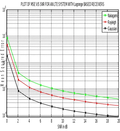
Fig. 12 MSE Vs SNR comparison plot of Lagrange interpolation

techniques for Nakagami, Rayleigh and Gaussian channel mobility

Figure 12 shows MSE vs SNR plot of Lagrange interpolation technique under the effect of Gaussian, Rayleigh and Nakagami fading channel for LTE system. Here, Lagrange interpolation technique gives better performance under the effect of Gaussian channel. Performance of Lagrange interpolation becomes poor for Rayleigh fading than Gaussian

0 2 4 6 8 10 12 14 16 18 20

10-3 10-2 10-1 100

SNR in dB

M e a n S q u a re d E rr o r

PLOT OF MSE V/S SNR FOR AN LTE SYSTEM UNDER RAYLEIGH FADING

Lagrange LS MMSE

0 2 4 6 8 10 12 14 16 18 20

10-3 10-2 10-1 100 101

SNR in dB

M e a n S q u a re d E rr o r

PLOT OF MSE V/S SNR FOR AN LTE SYSTEM under Nakagami Fading

Lagrange LS MMSE

0 2 4 6 8 10 12 14 16 18 20

10-4 10-3 10-2 10-1 100

SNR in dB

M e a n S q u a re d E rr o r

PLOT OF MSE V/S SNR FOR AN LTE SYSTEM WITH Lagrange BASED RECEIVERS

Nakagami Rayleigh Gaussian

0 2 4 6 8 10 12 14 16 18

10-2 10-1 100

SNR in dB

M e a n S q u a re d E rr o r

channel. And under the effect of Nakagami, Lagrange method gives worst MSE. Figure 13 shows MSE plot of LS and MMSE under the effect of mobility for LTE system. Here, MSE is plotted for 50Hz and 100Hz for LS, MMSE and Lagrange interpolation. It is seen that with mobility, mean square error is increased for LS and MMSE. Still MMSE performs better than LS under the effect of mobility. Lagrange interpolation method gives minimum MSE.

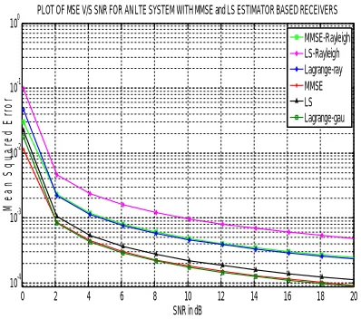
Fig. 14 MSE Vs SNR comparison plot of LS and MMSE for an LTE Fig. 15 MSE Vs SNR comparison plot of LS, MMSE and Lagrange

system under AWGN and Rayleigh fading with mobility and without method for LTE system under different multipath fading channel

mobility

Fig. 14 shows the comparison of LS and MMSE under the effect of AWGN and Rayleigh fading with and without mobility. It is seen that mobility gives higher MSE for LS and MMSE. So it degrades the performance of the system. Further, with zero mobility AWGN has less MSE than Rayleigh fading. Figure 15 shows the comparison of all the channel estimation techniques for LTE downlink system under different multipath fading channels-Gaussian, Rayleigh and Nakagami fading. Simulation results shows that among all the CE techniques, Lagrange polynomial interpolation performs better than all other for all multipath fading channels. Further, from the simulation results it is seen that among all three fading channels, AWGN has minimum MSE and Nakagami fading has higher MSE than other two.

VII. CONCLUSION

Here, LTE downlink channel is estimated under Gaussian channel, Rayleigh fading and Nakagami multipath fading channels by using LSE and MMSE estimation techniques with and without mobility. Further, to improve the channel efficiency Lagrange Polynomial Interpolation technique is proposed. From the simulation results, it is concluded that MMSE gives less MSE compared to LS for all three fading channels and also for with mobility. LSE is simple technique, whereas MMSE is complex because it includes auto correlation and cross-correlation functions. Proposed Lagrange Polynomial Interpolation technique offers a considerable improvement of the performance of Downlink LTE system. It makes the estimation more efficient and reduces the complexity of transceiver. By comparing all these techniques for different multipath fading-Gaussian, Rayleigh and Nakagami under the effect of mobility, it is concluded that Lagrange polynomial interpolation technique is much better than LS and MMSE. Moreover, it reduces the complexity of the transceiver. But mobility increases the MSE of the system for all the estimation techniques under all multipath fading channels. From all the simulation plots, it can be concluded that among all these multipath fading channels, we get minimum MSE under the effect of Gaussian channel and maximum MSE under Nakagami fading channel.

0 2 4 6 8 10 12 14 16 18 20

10-4 10-3 10-2 10-1 100

SNR in dB

M e a n S q u a re d E rr o r

PLOT OF MSE V/S SNR FOR AN LTE SYSTEM WITH MMSE and LS ESTIMATOR BASED RECEIVERS

MMSE-Rayleigh LS-Rayleigh Lagrange-ray MMSE LS Lagrange-gau

0 2 4 6 8 10 12 14 16 18 20

10-4 10-3 10-2 10-1 100

SNR in dB

M e a n S q u a re d E rr o r

COMPARISON PLOT OF MSE V/S SNR ALL FADING CHANNELS FOR AN LTE SYSTEM WITH MMSE,LS AND lAGRANGE ESTIMATOR

REFERENCES

1. Simone Morosi, Fabrizio Argenti, Massimiliano Baigini, Enrico Del Re “Comparison of Channel Estimation Algorithms for MIMO

Downlink LTE System” 9th International Wireless Communications and Mobile Computing Conference (IWCMC), IEEE, pp. 953 – 958,

July 2013.

2. Mallouki Nasreddine, Nsiri Bechir, Walid Hakimiand Mahmoud Ammar “Channel Estimation for Downlink LTE System Based on

LAGRANGE Polynomial Interpolation” The 10th _{International Conference on Wireless and Mobile Communications. IARIA 2014.}

3. Maulik J. Darji, Prof. Vanrajsinh B Vaghela “Channel Estimation for LTE Downlink using Various Techniques under the Effect of

Channel Length” IJSRD-International Journal for Scientific Research & Development, Vol.2, Issue 03, pp. 182-186, June 2014.

4. Bouchibane, F.Z., Ghanem, K. And Bensebti, M“Performance analysis of pilot pattern design for channel estimation in LTE downlink”

Antennas and Propagation Society International Symposium (APSURSI), IEEE, pp. 408-409, July 2014 .

5. Sinem coleri, Mustafa Ergen, Anuj Puri and Ahmad Bahai, “ Channel Estimation Techniques Based on Pilot Arrangement in OFDM

Syatems” IEEE Transactions on Broadcasting, Vol.48, Issue-.3, pp. 223-229, September 2002.

6. Muntadher Qasim Abdulhasan, Mustafa Ismael Salman, Chee Kyun Ng, Nor Kamariah Noordin “Approximate Linear Minimum Mean

Square Error Estimation Based on Channel Quality Indicator Feedback in LTE Systems” 11th Malaysia International Conference on

Communications, IEEE, pp.446 – 451, November 2013.

7. Liang Heng and Louay M.A. Jalloul “Performance of the 3GPP LTE Space–Frequency Block Codes in Frequency-selective Channels

With Imperfect Channel Estimation”, IEEE Transactions on Vehicular Technology, Vol. 64, Issue-5, pp.1848 – 1855, May 2015.

8. F.Z. Bouchibane, K. Ghanem, M. Bensebti, “Impact of Pilot Symbols Design on the Performance of the LTE System”, 1 st International

Conference on Electrical and Inforrnation Technologies (ICEIT) IEEE,pp-385 – 389, 2015.

9. Michel Simko, Di wu, Chritian Mehlfuhrer, John Eilert and Dake Liu “Implementation Aspects of Channel Estimation for 3GPP LTE

Terminals.” Proc. 17th _{European Wireless Conference (EW 2011), pp-1-5, April 2011.}

10. Sorna Keerthi R and Meena alias Jeyanthi K “Improved Channel Estimation Using Genetic Operators for LTE Downlink System”

International Conference on Science, Engineering and Management Research(ICSEMR) , IEEE, pp. 1-6, November 2014.

11. Li Tang, Zhu Hongbo “Analysis and Simulation of Nakagami Fading Channel with MATLAB*” In Proceeding Asia-Pacific Conference

on Environmental Electromagnetics, CEEM, pp.490-494, November 2003.

12. Rana M.M. “Channel estimation techniques and LTE terminal implementation challenges” 13th _{International Conference on Computer and}

Information Technology (ICCIT), pp. 545-549, December 2010.

13. Theodore S. Rappaport “Wireless Communications Princilples and Practice” 2nd _edition.

14. Houman Zarrincoub “Understanding LTE with Matlab”

BIOGRAPHY

Khushboo Arvindbhai Parmar is an M.E. student in the Electronics & Communication

Department, Sardar Vallabhbhai Patel Institute of Technology, Vasad, Gujarat, India. She received degree of B.E.in Electronics & Communication in 2010 from VNSGU, Surat, Gujarat, India. Her areas of interest are wireless communication system, wireless sensor networks, digital electronics and microwave engineering.

Prof. Saurabh M. Patel is an Asst. Professor in the Electronics & Communication Department,