R E S E A R C H
Open Access
Perceptually controlled doping for audio
source separation
Gaël Mahé
1*, Everton Z Nadalin
2, Ricardo Suyama
3and João MT Romano
2Abstract
The separation of an underdetermined audio mixture can be performed through sparse component analysis (SCA) that relies however on the strong hypothesis that source signals are sparse in some domain. To overcome this difficulty in the case where the original sources are available before the mixing process, the informed source separation (ISS) embeds in the mixture a watermark, which information can help a further separation. Though powerful, this technique is generally specific to a particular mixing setup and may be compromised by an additional bitrate compression stage. Thus, instead of watermarking, we propose a ‘doping’ method that makes the
time-frequency representation of each source more sparse, while preserving its audio quality. This method is based on an iterative decrease of the distance between the distribution of the signal and a target sparse distribution, under a perceptual constraint. We aim to show that the proposed approach is robust to audio coding and that the use of the sparsified signals improves the source separation, in comparison with the original sources. In this work, the analysis is made only in instantaneous mixtures and focused on voice sources.
Keywords: Informed source separation (ISS); Sparse component analysis (SCA); Doping watermarking; Sparsification
1 Introduction
Blind source separation (BSS) methods have been increas-ingly present in the signal processing literature since the first efforts in the area in the middle 80s. The BSS approach based on independent component analysis (ICA) is certainly consolidated as a fundamental unsuper-vised method [1], being employed especially in scenarios where the number of sources to be recovered is not greater than the number of sensors.
When dealing with the underdetermined case, i.e., sce-narios with more sources than sensors, methods usually associated with the idea of sparse component analysis (SCA) [1], which assume that the sources are sparse in some domain, are able to identify the mixing model or even, in some cases, perfectly separate the underlying sources [2].
Several SCA approaches explore the fact that source signals are disjoint in the time-frequency domain [3,4], which means that there are regions in the time-frequency domain in which there is at most one source active. These
*Correspondence: [email protected]
1LIPADE, Université Paris Descartes, Sorbonne Paris Cité, Paris 75006, France Full list of author information is available at the end of the article
methods operate in a similar fashion, performing the fol-lowing steps: (1) identify time-frequency regions in which at most one of the sources is active, (2) estimate the mixing parameters (or the direction of arrival (DOA)) associated with the active source, (3) gather all results in a histogram of estimates, and (4) process the histogram in order to obtain the mixing parameters (or the DOAs) and/or the number of sources [4-8].
If more than one source is active in each time-frequency region, but this number is smaller than the number of sensors, some methods try to identify the subspaces con-taining the sources and afterwards estimate the mixing parameters based on the information about these sub-spaces [9-11]. Another interesting approach is followed in [12] and [13], which combine SCA and ICA meth-ods, proposing that ICA be performed in time-frequency regions in which the number of active sources do not exceed the number of sensors.
It is important to mention that the performance of these methods, however, is strongly dependent on the key assumption that the source signals have a sparse repre-sentation in some given basis. In this sense, a different approach, the ‘informed source separation’ (ISS), was pro-posed [14]. In some particular audio applications, it is
possible to have access to the sources before the mixing process; for example, in a professional studio, the source signals are usually recorded separately and then mixed together to compose the final recording. Thus, one can embed at this stage additional information about the mix-ing process within the signals in an inaudible manner. This extra information can later be employed by the receiver to help recovering the sources and let the listener manipulate them separately.
For example, in [15], the time-frequency plane is divided in ‘molecules’ and the watermark information is either the energy contribution of each source to each molecule of the mixture or a coarse description of each molecule of each source. This watermark helps the separation of a linear instantaneous monophonic mixture of four or five sources. In the stereophonic case, [16] proposed to embed the information about the mixture matrix and, for each molecule, the index of the zero, one, or two dominating sources in the molecule. At the receiver’s end, thanks to this information, each molecule undergoes the separation process as a (over)determined mixture. Other methods [17-19] are described and evaluated in [14] that generally require the transmission of a compressed representation of the sources spectrograms and the mixing filters.
These methods achieve very good performance com-pared to BSS but require a considerable bit overhead (at least 5 kbit/s per source according to [14]). The com-patibility of the ISS with the current normalized formats implies to transmit this information through watermark-ing. Although high-capacity watermarking was recently proposed [20] for this purpose, it is dedicated to uncom-pressed formats (16 bits PCM) and would not be robust to bitrate compression.
This difficulty is overcome by the coding-based ISS approach [21], where the mixture and the sources are jointly coded. But in the context of audio broadcasting using standard compressed stereo formats, the water-marking approach should be chosen and the watermark should be robust to bitrate compression.
In an attempt to avoid the overhead inherent to ISS and the limitation regarding an additional coding step, we explored the concept of doping watermarking [22]. The principle is to imperceptibly change the properties of an audio signal in order to improve a particular processing task. For example, in [23], this idea was employed to ‘sta-tionarize’ audio signals, aiming to enhance acoustic echo cancelation; in [24], the authors proposed a ‘gaussianiza-tion’ procedure for non-linear system identification and [25] proposed a method for reducing the spectral support of the probability density function (PDF) of an audio sig-nal in order to match the conditions of the quantization theorem.
The method initially proposed in [22] aims at increasing the sparsity of the source signals without compromising
the perceptual audio quality, in order to enhance the per-formance of sparsity-based source separation methods [1]. Some issues remain however:
• Although it was experimentally shown that, for given parameters, this method sparsifies efficiently audio signals without audible distortion, the trade-off between sparsification and audio quality was not explored. In other terms, how sparse can we make the sources without audible distortion?
• The robustness of the sparsification against audio coding must be assessed.
• The improvement of source separation in [22] was studied only with regard to sources counting and sources direction estimation. The impact of the sparsification on the source separation itself should be studied.
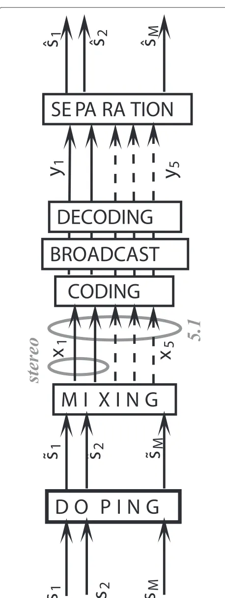
In this paper, we present a extension of this method that will deal with these issues. The studied scheme is repre-sented on Figure 1. We will focus on stereo mixtures of speech signals, which are a more homogeneous material than music and thus provide more easily reliable mean results from corpus of reasonable size.
As in [22], our goal is to imperceptibly sparsify the whole signal, although it would be possible to focus on the time-frequency bins where separation fails, which could distort less the signal for the same result in the separation process. This approach would however restrict the spar-sification of a signal to a given mixing scenario, which is another limitation of the ISS that we want to overcome. Our purpose is to facilitate the separation for any mixing scenario, i.e., without knowing in which time-frequency bins the separation will fail.
In order to expose our new methodology, the paper is organized as follows. In Section 2, we present a percep-tually controlled sparsification method, trying to increase the sparsity of the signals in the time-frequency domain but maintaining the same level of perceptual audio quality. Section 3 is dedicated to the impact of bitrate compres-sion on sparsity and vice-versa: how sparse signals remain after coding-decoding stages? How sparsification modi-fies the quality of coded-decoded signals? Finally, we study in Section 4 how the proposed sparsification improves source separation.
2 Sparsification 2.1 State of the art
Figure 1Doping watermarking scheme for audio source separation.Block diagram of the application considered in the present paper.
other frequency components (which is quite different from a masking threshold computed for coding or water-marking purpose, i.e., for noise addition). Each frequency component falling below this masking threshold shifted by some decibels (typically -6.6 dB), called ‘irrelevance func-tion’, is simply removed. According to the experimental results presented in [26], this method allows to remove around 36% of the Gabor coefficients, for sources sampled at 16 kHz.
However, as indicated by Balazs et al. [26], the Gabor scheme of analysis-synthesis implies overlapping synthe-sis windows with a high redundancy factor, which reduces the efficiency of the algorithm:‘components whose levels vary around the irrelevance threshold from one analysis interval to the next are not completely removed’. We ran a preliminary experiment of the irrelevance filter with the same masking model and an overlap-add scheme of analysis-synthesis (which was the one chosen in this paper), on a sequence of 5 s of speech sampled at 16 kHz. Although 32% of the TF coefficients can be removed (an amount similar to that found by Balazs et al. [26], a time-frequency analysis of the filtered signal exhibits almost the same histogram of the TF coefficients as the original signal, with the same amount of coefficients near zero.
To overcome this drawback, the principle of the irrel-evance filter was revisited by [27], in the framework of modified discrete cosine transform (MDCT)-based analysis-synthesis. This scheme avoids the effects of over-lapping in the temporal reconstruction. In other words, going back to the TF representation of a sparsified signal gives again exactly the MDCT resulting from the irrele-vance filter, so that the amount of zeroed TF coefficients remains the same.
The algorithm of [27] reaches ca. 75% of the coeffi-cients set to zero without audible distortion. Note that this result was obtained with audio signals sampled at 44.1 kHz, where a larger amount of frequential compo-nents are inaudible than in 16 kHz-sampled signals. This method was used as a pre-processing step in the ISS algo-rithm described in [16], which applies an ICA algoalgo-rithm to each TF bin of a stereo mix, based on the assumption that there are at most two dominating sources in each bin. Since this sparsification increases the amount of TF bins without any active sources, which do not need to be separated, it reduces the computational complexity of the separation. Nevertheless, as pointed out by the authors, this sparsification procedure leads to a small improvement in separation quality because the bins for which a perfect separation is possible (zero to two sources) represent only 10% of the energy of the mix in the presented experiments, with mixtures of five sources each (real music tracks).
does not provide satisfactory results. Instead of the binary sparsification proposed by the latter, a ‘smooth’ sparsifi-cation, robust to the inter-blocks effects of the temporal reconstruction, was proposed in [22].
The sparsification described in [22] is based on a para-metric approach of the source TF coefficients distribution. Denoting by|S(m,f)|the TF coefficients (in modulus) of an audio signals, their distribution can be approximately modeled by a generalized Gaussian distribution, with a form factor β varying between 0.2 and 0.4 [28]. Thus, the idea is to design a time-varying filter that will trans-form the original sources(n)into a new signal˜s(n), such that its time-frequency coefficients modulus|˜S(m,f)|are also distributed according to a generalized Gaussian dis-tribution but with a smaller form factorβ. In this sense, the probability density function of the filtered signal time-frequency coefficients modulus should be equal to
ftarget(|˜S(m,f)|)=
withα denoting the scale factor of the original distribu-tion, in order to maintain the same variance as the original signal.
The sparsifying method can be summarized as follows:
1. Compute the time-frequency representationS(m,f), using non-overlapping windows of 32 ms.
2. Estimate the form factorβof the distribution of
|S(m,f)|, assuming a generalized Gaussian distribution.
3. For a fixed target form factorβ< β, obtain the target time-frequency representation as
|˜S(m,f)| =Ftarget−1 Femp(|S(m,f)|) (3)
whereFemp(.)denotes the empirical cumulative distribution of|S(m,f)|andFtarget(.)the target cumulative distribution.
4. For each frame, obtain the sparsifying filter frequency response as
H(m,f)= |˜S(m,f)|
|S(m,f)| (4)
and apply it to each time frame.
It was shown experimentally that this method effi-ciently sparsifies speech signals, while preserving a good audio quality. This sparsification led to better results in
SCA, concerning the estimation of the number of sources present in a mixture and the estimation of the mixing matrix. However, the method does not ensure in itself the preservation of the audio quality. Hence, the ques-tion of the tradeoff between the sparsificaques-tion and the audio quality remains open. In other terms, how could we make an audio signal as sparse as possible, while keeping it perceptually unchanged?
2.2 Perceptually controlled sparsification
The perceptual cost of the previous algorithm could be reduced by procesing each frequency bin independently, i.e., in each frequency bin reducing the form factor of the distribution while keeping the variance unchanged. Since the range of TF coefficients strongly depends on the frequency, this would avoid the risk of excessive modifi-cation of the variances due to processing the whole TF plane globally. However, in this framework, we consider instantaneous mixtures, for which the separation is per-formed using the whole signal. Consequently, the sparsity is required for the distribution of the whole TF plane, so that we chose to base the sparsification on the distribution of all TF coefficients of the whole signal, while ensuring the perceptual control by other means.
Following the same framework as in [22], our goal is to find a transformation of the spectrogram|S(m,f)|into |˜S(m,f)|so that the empirical distribution of the latter,f|˜S|, is as close as possible toftarget, while the modified signal˜s is perceptually equivalent to the original signals. This may be expressed by the following optimization problem:
min d(f|˜S|,ftarget) under the constraint: dpercept(s,s˜) <dth (5)
where d is a distance between distributions (for example the Kolmogorov-Smirnov distance, denoted by dKSin the following), dperceptis a perceptual distance between audio signals anddthis the audibility threshold for this distance. We propose to solve this problem in an iterative way, i.e., by reducing step by step dKS(f|˜S|,ftarget) while keep-ing dpercept(s,˜s) < dth. Initially,|S˜| = |S|andH(m,f) = 1 ∀(m,f). For each time-frequency bin (m,f), we shift |˜S(m,f)|according to the goal of reducing dKS(f|˜S|,ftarget), under the constraint dpercept(s,˜s) < dth. This pro-cedure is repeated until f|˜S| is close enough to ftarget (i.e., dKS(f|˜S|,ftarget) lower than a given threshold ε) or dpercept(s,˜s)reachesdth(see Algorithm 1).
The rule for shifting |˜S(m,f)| is based on a compar-ison between the values of the cumulative distribution functionsF|˜S| andFtarget in a neighborhood of|˜S(m,f)|. Considering an arbitrary small value in dB, if F|˜S|
Algorithm 1Iterative modification of the histogram of the
dpercept>dth¯ ∨ number of iterations>MAX_IT
10/20|˜S(m,f)|[), then HdB(m,f) decreases (resp. increases) of (in dB), as well as |˜S(m,f)|dB. Conse-quently,|F|˜S|−Ftarget|decreases on the intervalI.
Since the Kolmogorov-Smirnov distance is the max of |F|˜S|−Ftarget|onR, it decreases if this max belongs to the intervalI or remains constant otherwise. The proposed rule does not ensure a strict decrease of dKS(f|˜S|,ftarget) at each step, but it reduces step by step the difference betweenF|˜S| and Ftarget, which contributes, in the long term, to a decrease of dKS(f|˜S|,ftarget).
The choice ofdetermines the convergence.
We experimentally observed that higher values can speed up the decrease of the distance to minimize, but too large values make the condition for shifting more difficult to verify, which may stop the algorihtm before its conver-gence or at least slow it down. Note that the algorithm is sensitive to the order in which the TF bins are processed. Choosing a smaller value for reduces this sensitivity. Finally, the value ofinfluences the audio quality of the
transformed signal since too high values may cause an audible spectral distortion.
Differences between neighboring binsH(m,f)have also an impact on the audio quality. We observed experimen-tally that letting each bin evolve independently from its neighbors leads to an audible distortion: the sound is per-ceived as ‘robotic’. Thus, we fixed an additional condition for shiftingH(m,f)and|˜S(m,f)|: the difference between two neighboring bins HdB(m,f) should not exceed an arbitrary thresholdfreqmax(f) in the frequency dimension andtimemax(f)in the time dimension. These values depends on the frequency sensitivity of the ear that depends on the frequency.
Many objective perceptual distances between audio sig-nals were proposed in the literature [29], with various complexities and correlations with the real perception. In our case, i.e., a spectral distortion caused by filtering, the Bark spectral distortion (BSD) [30] was shown to be well correlated with the perceived distortion of speech signals [29] and its complexity is moderate. Thus, it is an adequate perceptual distance here.
For two signalssand˜s(distorted version ofs), for each frame m, the power spectra are converted in loudness spectra, representing the perceived loudnesses, in Sones, on a Bark frequency scale, using a basic psychoacoustic model. Hence, the spectrograms ofsand˜sresult in loud-ness spectrogramsSs(m,b)andS˜s(m,b), respectively. The normalized local BSD for a framemis defined as:
BSD(m)=
whereNbis the number of considered critical bands. The global BSD for the whole signal is the mean of the local BSDs.
In the proposed algorithm, we chose the BSD as percep-tual distance and fixed two thresholds: one for the global BSD of the distorted signal, denoted byd¯th, and another for the local BSD of each frame, denoted bydth, greater thand¯th.
2.3 Implementation in the time domain
2.4 Experimental results
In this experiment as well as in the following ones, the estimation of the distributions and the sparsification is performed only on the non-silent parts of the signal. The form factors are estimated by the moments method [31].
As in [22], we set the target form factor at half of the original one.
We fixed = 0.2 dB and freqmax(f) according to the frequential sensivity of the ear, which is constant below 500 Hz and decreases beyond 500 Hz. Hence, we set freqmax(f) proportional to the width of the critical bands, i.e., inversely proportional to the derivative db/df, where
bdenotes the Bark frequency, which can be approximated by [29]:
b=sinh−1(f/600) (7)
Thus, we get:
freqmax(f)=0
(f/600)2+1 (8)
where 0is fixed to 3 dB. The value oftimemax(f) is less critical, in particular because of the inter-frames smooth-ing in the temporal implementation of the filter. We fixed timemax(f)=4freqmax(f).
Concerning the stop criteria, we fixed ε = 10−4 and dth = 1. Whereas we observed that the algorithm is not very sensitive to dth, the final quality depends crucially ond¯th. In preliminary experiments, we output the spar-sified signal ˜s at each iteration and estimated its mean opinion score (MOS) compared to the original signal s
by PESQ [32]. For any source, the MOS decreases as the global BSD increases, unsurprisingly. But the relationship between the MOS and the BSD is not the same for all sources, which makes difficult to fix a BSD threshold cor-responding to the inaudibility threshold for any source. Consequently, the optimal BSD threshold d¯th has to be learned on a training corpus.
2.4.1 Training corpus
The training corpus was constituted from the TIMIT database [33] in the same manner as the test corpus used in [22] but with different speakers. The corpus is composed of 32 source signals, each consisting in three sentences pronounced by the same speaker (32 different speakers), sampled at 16 kHz, truncated to 5 s.
The algorithm was run on this training corpus, with the following stop criteria:d¯th= ∞, MOS=3.5, MAX_IT= 200. As shown by Figure 2, the relationship between MOS and BSD is very variable. However, according to these results, fixing d¯th = 0.12 should provide a good MOS (≥4) for most of the sourcesa.
Figure 2MOS/BSD relationship.Each line represents, for one of the 32 sources of the training corpus, the trajectory of the pair (BSD, MOS) during the sparsification process. For all the sources, the first point is (0, 4.64), but as soon as the second point (end of the first iteration), the MOS is very variable according to the source.
2.4.2 Test corpus
The test corpus is the same as that used in [22], with 96 different speech sources of 5 s. In this experiment, the MOS was not output at each iteration and we fixed the fol-lowing stop criteria:ε = 10−4,d¯th = 0.12,dth = 1, and MAX_IT=100.
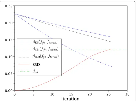
As an example, Figure 3 displays the convergence of the algorithm in terms of Kolmogorov-Smirnov distance, in parallel with the Bark spectral distortion, for one of the source signals, which original form factor is 0.32. At the end of the algorithm, the form factor of the spectrogram
Figure 3Convergence of the sparsification algorithm.For a 5-s speech signal, evolution of the Kolmogorov-Smirnov distance (dKS),
the Cramér-von Mises distance (dCM), and the chi squared distance
(dchi squared) betweenf|˜S|andftarget, in parallel with the Bark spectral
distribution is 0.24 and the MOS is 4.5. The original and sparsified distributions are represented on Figure 4.
Figure 3 displays also two other distances between the empirical and the target distribution, which evolution show the robustness of the algorithm to the choice of the distance. They were normalized so that their first value matches that of dKS.
The Cramér-von Mises distance (dCM) measures a Euclidian distance between the empirical and the target cumulative distributions, defined as:
dCM(f|˜S|,ftarget)= 1 12N +
N
i=1
2i−1
2N −Ftarget(Xi)
2
(9)
whereNis the number of TF coefficients and(Xi)1≤i≤N denotes the ordered sequence of the TF coefficients |˜S(m,f)|. Unsurprisingly, this distance decreases, since the algorithm is based on a decrease of|F|˜S|−Ftarget|on small intervals.
The chi squared distance (dchi squared) is based on a com-parison between the distributions themselves. Since the empirical distribution is discrete whereas the theoritical distribution is continuous, the distance is quantile-based. We definerintervals(Ii)1≤i≤r, containing approximately the same number of coefficients |˜S(m,f)|. Denoting by P|˜S|(Ii) andPtarget(Ii), respectively, the empirical and the target probabilities of the ith interval, the chi squared distance is defined as:
dχ2(f|˜S|,ftarget)=
r
i=1
P|˜S|(Ii)−Ptarget(Ii) 2
Ptarget(Ii)
(10)
We choser=1, 000. This distance decreases in the same manner as the others.
Figure 4Original and sparsified distributions.Zoom on a part of the distributionf|S˜|of the sparsified signal after convergence, compared to the original onef|S|.
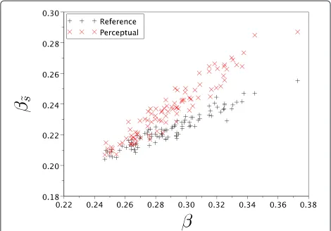
For the whole corpus, Figure 5 shows for both algo-rithms (this one, calledperceptual, and [22], called refer-ence) the couples(β,β˜s), where for each source signalβ denotes the original form factor and β˜s the form factor of the sparsified signal. The latter was computed from a time-frequency analysis of the sparsified signalafterthe reconstruction in the time domain. The time-frequency analysis was based on the same segmentation as for the original signal. The sources are slightly less sparsified with the proposed algorithm, but thanks to the perceptual con-trol, the audio quality is ensured (see Figure 6): only 1 of the 96 sparsified speech sources have a MOS lower than 4 and 80% of the sparsified signals have a MOS greater than or equal to 4.4. The mean MOS on the corpus is 4.4 instead of 4.1 with the previous algorithm [22]. A chi squared test of similarity between the previous distribu-tion of the MOS values and this distribudistribu-tion, with classes of width 0.1, provides a p value of 9.6 × 10⁻³, which indicates that the distributions are significantly different. Figure 7 illustrates the trade-off sparsity/quality, compar-ing the proposed algorithm to the reference algorithm [22].
2.4.3 Robustness to time/frequency operations
One could wonder if the obtained form factors are differ-ent from these computed directly after the sparsification in the frequency domain, before the time-domain recon-struction. In other terms, since this step was a critical issue in the sparsification method of [26], what is the effect of the synthesis through the overlap-add method?
The mean values of the form factors before and after the time-domain reconstruction are, respectively, 0.2315 and 0.2366. Assuming a normal distribution of the form
Figure 5Estimated form factor of the sparsified signal vs estimated form factor of the original signal.Estimated form factor
Figure 6Histograms of the estimated MOS of the sparsified signals.Histograms of the estimated MOS of the sparsified signals, for the reference algorithm [22] and the proposed algorithm.
factors, a Student test indicates apvalue of 0.051. Hence, the difference between the mean values is weak com-pared to the sparsity improvement and weakly significant. We can conclude that our sparsification is robust to the overlap-add synthesis.
Another question is the robustness of the sparsity to the frame desynchronization between the transmitting and the receiving part of the communication chain. Since the system is more intended for file transfer than for broadcast, this question is not a critical issue: the beginning of the file remains the same and the frame length can be transmitted through the metadata of the file header. Consequently, we just tested this issue for one speaker of the corpus.
Figure 7Audio quality vs sparsity.For each of the 96 sources, estimated MOS vs form factorβ˜sof the sparsified signal. Comparison between the previous algorithm [22] (refered asreference) and the proposed algorithm (refered asperceptual).
For this speaker, the original form factor of the spectro-gram computed with non-overlapping frames of 32 ms is 0.26 and the sparsification leads to a form factor of 0.22. Shifting the time-frequency analysis of the sparsified sig-nal of 16 ms (half of a frame) increases the form factor of only 0.004. Choosing another frame length for the analy-sis (respectively, 16 and 64 ms) modifies the form factor of the original signal (respectively, 0.30 and 0.24) and the form factor of the sparsified signal (respectively, 0.24 and 0.21) in the same way, so that the sparsified signal is kept sparser than the original one.
3 Quality and sparsity of sparsified coded signals We have proposed a sparsification algorithm that reduces the form factor of the generalized Gaussian model of the source distribution, while preserving the audio quality. Nevertheless, as indicated in Figure 1, a more realis-tic scenario should also consider the possible distortion introduced by a coding scheme. In this section, we will consider two codecs: the GSMb [34], which is intended for speech and allows to test the effect of a deep mod-ification of the signal; the MP3c [35], since it includes natively a stereo mode (unlike GSM) and is more appro-priate for the future extention of this work to music signals.
3.1 Robustness of the sparsity against coding
To test how sparse signals remain after coding-decoding, we coded each source signal separately, as well as its spar-sified version. Hence, the MP3 codec works on mono mode, with a bitrate of 96 kbps, known to provide a transparent quality for mono signals. Figure 8 shows the couples (β,βcodec), for the original and the sparsi-fied signals, in both coding cases, where β and βcodec denote the form factors of respectively the uncoded and the coded-decoded signal. The coding-decoding process causes almost no variation of the form factors in the MP3 case and a very small variation in the GSM case, even neg-ative. Hence, speech coding, even with a low bitrate, does not alter the sparsity of the signals.
3.2 Quality of the coded sparsified signals
As in Section 2, we used PESQ to estimate the per-ceived audio quality. In the practical scheme presented in Figure 1, the quality should be measured on various mix-tures after decoding. But since PESQ is not validated for a mixture of speech signals, we only measured the quality for each source signal coded separately. In the GSM case, the MOS were estimated using 8 kHz sampled signals, since the GSM works only at this frequency.
For each source signal, taking as reference the original signal, we computed two values:
• The MOS of the coded-decoded version of the original signal
• The MOS of the coded-decoded version of the sparsified signal
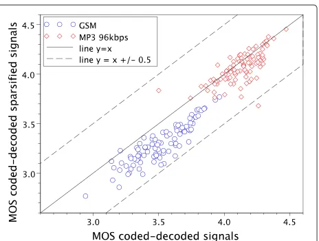
As shown by Figure 9,
• In the MP3-coding case, the impairment due to the sparsification is small compared to this due to the coding.
Figure 9Impact of sparsification on the quality loss due to coding.MOS variation due to the sparsification: taking in both cases the original signals as references, MOS of the coded-decoded sparsified signals vs MOS of the coded-decoded signals, for GSM and MP3 coding.
• In the GSM-coding case, the sparsification increases slightly the impairment due to the coding.
Note that we discarded two outliers in the MP3 case, with coordinates (1.75,4.23) and (2.51,4.15). In both orig-inal signals, there was a slight whistling, which caused an artefact in the coded signals. The sparsification smoothed this artefact, so that the quality is good for the decoded sparsified signal, whereas it is poor for the coded-decoded signal.
4 Separation of mixtures of sparsified signals 4.1 Methods
In SCA approaches, source separation techniques are usu-ally divided in three steps: (i) identification of the number
Figure 8Robustness of the sparsity against coding.Form factorsβcodecof the coded-decoded signals vs form factorsβof the uncoded signals
of sources in the mixtures, (ii) identification of the mixing system, and (iii) source separation itself. In this section, we verify the performance of each aforementioned step when the doping watermarking procedure is employed. For the first two steps, we will use the ICA-SCA based approach proposed in [13,36] that was also used in [22]. In a stereo mixing situation, the algorithm can be summarized as follows:
1. Compute FFT of the mixing signals using the same parameters as in the sparsification process. 2. Divide the FFT data in blocks and for each block
apply ICA to the mixing signals, assuming that there are two or less sources active in the block. The ICA method will provide a ‘local separation matrix’W2×2. 3. Compute and store all the anglesθi(two for each
block) obtained by:
θi=tan−1[W −1]
2,i
[W−1]1,i,i=1, 2. (11)
4. Apply K-means [37], or other clustering method inθ, to find the number of clusters that better fits the data. This number will be the amount of sources present in the mixture.
5. The centroid of each cluster indicates a value ofθ that will be related to the direction of one of the columns of the global mixing matrix.
Finally, after estimating the mixing matrix, we used the flexible audio source separation toolbox (FASST) [38] to separate the sources. This comprehensive toolbox con-tains some of the most common approaches of audio source separation. A set of prior constraints and a decom-position based on local Gaussian modeling of the sources are used to find which framework is more suitable to separate each set of sources. In this work,
• The mixture is stereo, instantaneous, and underdetermined in most of the cases.
• The STFT was used for signal representation, and the mixing parameters were estimated using the
SCA/ICA approach presented in [13]d, giving GEM algorithm a ‘good initialization’. The parameters settings used in FASST correspond to the
multichannel NMF method presented in [39] in the instantaneous case.
In the following experiments, each step is run with the perfect estimation of the previous step, in order to study separately the impact of the sparsification on each part of the source separation.
4.2 Experimental results
In order to verify the improvement provided by the pro-posed sparsification method in each of the three steps of the source separation, we proposed some simulation
scenarios. In each of them, the algorithms were run 100 times and results are an average of them. In each case, the sources were randomly chosen among the 96 speech sig-nals of the test corpus described earlier. The number of sources in the mixtures varied from two to six, and only stereo mixtures were considered. The FFT window had 512 samples and an overlap of half window. All the tests were made with 1- and 5-s sampled sources. The mixing matrix was the same in all the runs and its directionsθ were chosen to be equally spaced.
4.2.1 Estimation of the number of sources
In this first scenario, we applied the fourth step of the aforementioned algorithm in order to estimate the num-ber of sources. In the case of samples with 5 s, considering both cases - original sources and sparsified sources - all simulations found the correct number of sources.
With 1-s samples, the sparsification procedure was able to reduce the estimation errors when the number of source is higher than 2. Using the original sources, the estimation errors are 0%, 2%, 2%, 8%, and 11%, for two, three, four, five, and six sources, respectively. However, when the sparsifcation procedure is employed, the estima-tion errors are 1%, 0%, 0%, 5%, and 9%, for two, three, four, five, and six sources, respectively.
4.2.2 Estimation of the mixing matrices
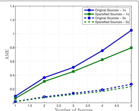
Considering now that the number of sources was cor-rectly found, we applied the fifth step of the aforemen-tioned algorithm to estimate the direction of each column of the mixing matrix. We computed the angular mean error (AME) between the directions θ of the mixing matrix A and its estimation. The results presented in Figure 10 show that sparsification was able to reduce the
Table 1 Source separation results for 1 s of speech
No. of sources SDR (dB) SDRsparse (dB) SIR (dB) SIRsparse (dB) SAR (dB) SARsparse (dB)
2 50.4 49.9 60.4 59.8 51.5 51.2
3 14.0 15.1 18.6 19.8 16.3 17.5
4 9.5 10.7 13.5 14.7 12.2 13.4
5 5.8 6.6 9.1 9.8 9.7 10.7
6 3.5 4.5 6.5 7.3 8.2 9.3
SDR, SIR, and SAR for original and sparsified signals. Mean values of 100 simulations with 1-s speech signals.
AME, being even more effective as the number of sources increases.
4.2.3 Source separation
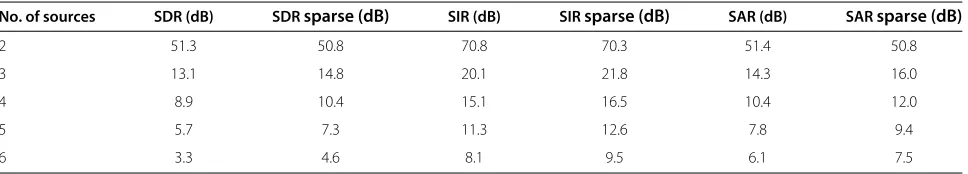
With the same configuration, but now assuming that both the number of sources N and the mixing matrixA are known, the source separation was performed using the FASST algorithm. Tables 1 and 2 (for 1- and 5-s sources, respectively) show the result of signal-to-distortion ratio (SDR), interference ratio (SIR), and signal-to-artifact ratio (SAR), calculated as described in [40].
For the sparsified signals, these metrics were computed taking as references the sparsified signals. Since the goal of the proposed scheme is to objectively distort the original sources while maintaining them perceptually unchanged, taking the original sources as references would lead to a meaningless distortion of objective metrics like SDR, SIR, and SAR, masking the performance of the source separation algorithm. This choice has the further advan-tage of assessing the performance of each processing step separately.
Observing the values obtained for the sparsified sources (correspond to the values SDRsparse, SIRsparse, and SAR
sparsein Tables 1 and 2), the gain found for the proposed scheme, except for the case with two sources, is around 1.5 dB for 5-s samples, and around 1.2 dB for 1-s samples, for the three ratios. For two sources, we are operating in a condition in which it is possible, in theory, to perfectly recover the original signals, and therefore the use of the sparsification does not significantly change the separation results - the three ratios are around 50 dB, indicating a good source recovery.
We also tested the proposed methodology using per-ception evaluation methods for audio source separation
(PEASS) toolkit [41], which describes a set of four per-ceptual scores (PS): overall (OPS), target-related (TPS), interference-related (IPS), and artifacts-related (APS), generated through a nonlinear mapping of the PEMO-Q auditory model [42]. Figure 11 shows the results of OPS, TPS, IPS, and APS for the 5-s sources, for the separation of the signals without sparsification (‘Normal’), the sepa-ration of the sparsified signals using the sparsified signals as reference signals (‘Sparsified’), and using the original sources as reference signals (‘Original as ref ’). The use of the original signals as reference would, in theory, give us an overall subjective performance.
Using the sparsified signals as reference, one can observe that there is an improvement using the sparsified sources in some cases, but the difference between the scores obtained when no sparsification procedure is employed and with the proposed sparsification method is small.
When the original sources are used as reference signals, three of the scores show that the performance of the pro-posal does not meet the expectations, the only exception being the TPS results, for which the proposed method presents a significant improvement in scenarios with a large number of sources. These results can be explained by the fact that the processing steps performed until the sources have been estimated introduce two percep-tual impairments: one due to the sparsification procedure (which is inaudible as a single step) and one due to the separation step, since we are operating, in most of the simulated cases, in an underdetermined mixture scenario. Nevertheless, it should be mentioned that PEASS is not intended to evaluate distortions like those introduced by the sparsification process, and therefore the evaluation of the cumulative effect of the perceptual impairments may not be completely reliable.
Table 2 Source separation results for 5 s of speech
No. of sources SDR (dB) SDRsparse (dB) SIR (dB) SIRsparse (dB) SAR (dB) SARsparse (dB)
2 51.3 50.8 70.8 70.3 51.4 50.8
3 13.1 14.8 20.1 21.8 14.3 16.0
4 8.9 10.4 15.1 16.5 10.4 12.0
5 5.7 7.3 11.3 12.6 7.8 9.4
6 3.3 4.6 8.1 9.5 6.1 7.5
Figure 11Source separation subjective results for 5 s of speech. OPS, TPS, IPS, and APS for original and sparsified signals (sparsified and original sources used as reference). Mean values of 100 simulations with 5-s speech signals.
4.3 Robustness to coding
As explained before, one disadvantage of traditional ISS approaches is that the watermarking information can be corrupted due to a signal compression. The robust-ness of the proposed sparsification to compression (see Subsection 3.1) let expect that the separation should also be robust. In order to verify it, an MP3 coding was consid-ered in the simulations, following the application diagram block depicted in Figure 1, at a bitrate of 192kbit/s. The configuration of the simulations is the same as described before.
When the number of sources are estimated, both orig-inal and sparsified sources generated exactly the same results. For the estimation of the mixing matrices, there were no significant difference for 1-s sources and the bet-ter performance achieved for the sparsified 5-s sources was maintained but with smaller differences among the results.
For the source separation, the results are very similar both using and not using the MP3 coding. For example, Table 3 shows the results of SDR, SIR, and SAR using
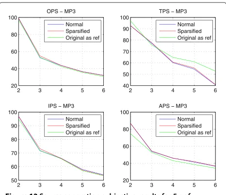
Figure 12Source separation subjective results for 5 s of MP3-coded speech.OPS, TPS, IPS, and APS for original and sparsified signals (sparsified and original sources used as reference). Mean values of 100 simulations with 5-s speech signals.
the 5-s samples, and Figure 12 shows the results for the perceptual evaluation.
5 Conclusions
We have proposed a doping process that makes audio signals more sparse while preserving their audio quality, thanks to a perceptually controlled algorithm based on a generalized Gaussian model of the time-frequency coef-ficients. This built sparsity is robust to compression and leads to an improvement of source separation.
Although the improvement of SDR, SIR, SAR, and even of the perceptual evaluation metrics is weak compared to usual results of ISS (1 to 2 dB instead 5 to 20 dB in [14] for the objective metrics), this method has two advantages: it is robust to compression, and the sparsification of each source is valid for any mixture, whereas the information watermarked in ISS is specific to one particular mixture.
Relaxing this specification could however allow to pro-cess only the time-frequency bin where the separation fails and hence potentially improve the separation for the same quality of the sparsified sources.
Table 3 Source separation results for 5 s of MP3-coded speech
No. of sources SDR (dB) SDR sparse (dB) SIR (dB) SIR sparse (dB) SAR (dB) SAR sparse (dB)
2 30.3 33.3 53.0 55.8 30.4 33.3
3 13.2 14.8 20.4 22.0 14.4 16.0
4 9.0 10.4 15.2 16.5 10.5 12.1
5 5.8 7.3 11.2 12.7 7.8 9.5
6 3.3 4.8 8.1 9.4 6.1 7.6
Beyond classical indices as SDR, SIR, and SAR (or their perceptual equivalents provided by PEASS) that evalu-ate the quality of each separevalu-ated source individually, the proposed method should be evaluated in the context of remixing that ISS is intended to. A specific protocol must be designed to evaluate the quality of mixtures of the sep-arated sources where various new mixing matrices are applied.
The proposed sparsification was experimentally val-idated on speech, which has the advantage of being a homogeneous test material. Further studies should enlarge the study to music that is the original application of ISS.
Endnotes
aAccording to [32], PESQ provides scores between 1
(very annoying impairment) and 4.5 (no perceptible impairment). Actually, the software provided by the ITU yields a maximum score of 4.64.
bWe used the GSM conversion of sox
(|http://sox.sourceforge.net|)., which
implements the version 06.10 of GSM. cWe used the codec LAME 3.98.3
(|http://lame.sourceforge.net|).
dIt should be mentioned that FASST is able to estimate
the signals even if this information is not available. Nevertheless, after some simulations, it could be noted that the estimation performance is clearly improved if such information is provided to the FASST method.
Abbreviations
AME: angular mean error; BSD: Bark spectral distortion; BSS: blind source separation; ICA: independent component analysis; ISS: informed source separation; MOS: mean opinion score; PCM: pulse-code modulation; PDF: probability density function; PESQ: perceptual evaluation of speech quality; SAR: signal-to-artifact ratio; SCA: sparse component analysis; SDR: signal-to-distortion ratio; SIR: signal-to-interference ratio; TF: time-frequency.
Competing interests
The authors declare that they have no competing interests.
Acknowledgements
The authors would like to thank CNPq, FAPESP (process no.2012/08212-4), and CAPES-COFECUB (project no. Ph 772-13) for the financial support.
Author details
1LIPADE, Université Paris Descartes, Sorbonne Paris Cité, Paris 75006, France. 2DSPCom Lab, School of Electrical and Computer Engineering (FEEC), University of Campinas, Campinas, SP 13083-970, Brazil.3Centro de Engenharia, Modelagem e Ciências Sociais Aplicadas (CECS), Universidade Federal do ABC (UFABC), Santo André 09210-170, Brazil.
Received: 1 July 2013 Accepted: 11 February 2014 Published: 4 March 2014
References
1. P Comon, P Jutten,Handbook of Blind Source Separation(Academic Press, Oxford, 2010)
2. S Rickard, Sparse sources are separated sources, inProceedings of the 14th Annual European Signal Processing Conference(Eurasip, Florence Italy, September 2006)
3. O Yilmaz, S Rickard, Blind separation of speech mixtures via time-frequency masking. IEEE Trans. Signal Process.52(7), 1830–1847 (2004)
4. S Arberet, R Gribonval, F Bimbot, A robust method to count and locate audio sources in a multichannel underdetermined mixture. IEEE Trans. Signal Process.58, 121–133 (2010)
5. JD Xu, XC Yu, D Hu, LB Zhang, A fast mixing matrix estimation method in the wavelet domain. Signal Process.95(0), 58–66 (2014). [http://www. sciencedirect.com/science/article/pii/S0165168413003241] 6. D Pavlidi, A Griffin, M Puigt, A Mouchtaris, Real-time multiple sound
source localization and counting using a circular microphone array. IEEE Trans. Audio Speech Lang. Process.21(10), 2193–2206 (2013) 7. S Araki, T Nakatani, H Sawada, Simultaneous clustering of mixing and
spectral model parameters for blind sparse source separation, in2010 IEEE International Conference on Acoustics Speech and Signal Processing (ICASSP), Piscataway: IEEE; 2010:5–8 (Dallas USA, March 2010)
8. G Zhou, Z Yang, S Xie, JM Yang, Mixing matrix estimation from sparse mixtures with unknown number of sources. IEEE Trans. Neural Netw.
22(2), 211–221 (2011)
9. MN Syed, PG Georgiev, PM Pardalos, A hierarchical approach for sparse source Blind Signal Separation problem. Comput. Oper. Res.41(0), 386–398 (2014). [http://www.sciencedirect.com/science/article/pii/ S0305054812002699]
10. JJ Thiagarajan, KN Ramamurthy, A Spanias, Mixing matrix estimation using discriminative clustering for blind source separation. Digit. Signal Process.23, 9–18 (2013). [http://www.sciencedirect.com/science/article/ pii/S1051200412001716]
11. FM Naini, GH Mohimani, M Babaie-Zadeh, C Jutten, Estimating the mixing matrix in Sparse Component Analysis (SCA) based on partial
k-dimensional subspace clustering. Neurocomputing.71(10-12), 2330–2343 (2008). [http://www.sciencedirect.com/science/article/pii/ S0925231208001033]. [Neurocomputing for Vision Research Advances in Blind Signal Processing]
12. F Nesta, M Omologo, Generalized state coherence transform for multidimensional TDOA estimation of multiple sources. IEEE Trans. Audio Speech Lang. Process.20, 246–260 (2012)
13. EZ Nadalin, R Suyama, R Attux, An ICA-based method for blind source separation in sparse domains, inProceedings of the 8th International Conference on Independent Component Analysis and Signal Separation (ICA 2009)(ICA Research Network Paraty, Brazil, March 2009), pp. 597–604 14. A Liutkus, S Gorlow, N Sturmel, S Zhang, L Girin, R Badeau, L Daudet, S
Marchang, G Richard, Informed Source Separation: a Comparative Study, inProceedings European Signal Processing Conference (EUSIPCO 2012) (Eusipco Bucharest, Romania, August 2012)
15. M Parvaix, L Girin, J Brossier, A watermarking-based method for informed source separation of audio signals with a single sensor. IEEE Trans. Audio Speech Lang. Process.18(6), 1464–1475 (2010). [http://hal.archives-ouvertes.fr/hal-00486809]
16. M Parvaix, L Girin, J Brossier, Informed source separation of linear instantaneous under-determined audio mixtures by source index embedding. IEEE Trans. Audio Speech Lang. Process.19(6), 1721–1733 (2011)
17. A Liutkus, J Pinel, R Badeau, L Girin, G Richard, Informed source separation through spectrogram coding and data embedding. Signal Process.92(8), 1937–1949 (2012)
18. S Gorlow, S Marchand, Informed Source Separation: Underdetermined Source Signal Recovery from an Instantaneous Stereo Mixture, in Proceedings of the 2011 IEEE Workshop on Applications of Signal Processing to Audio and Acoustics (WASPAA 2011)(IEEE New Paltz, USA, October 2011), pp. 309–312. [http://hal.archives-ouvertes.fr/hal-00646276] 19. N Sturmel, L Daudet, Informed source separation using iterative
reconstruction. IEEE Trans. Audio Speech Lang. Process.21, 178–185 (2013)
20. J Pinel, L Girin, A high-rate data hiding technique for audio signals based on IntMDCT quantization, inProceedings of the DAFx Conference(IRCAM Paris, France, September 2011), pp. 353–356. [http://hal.archives-ouvertes. fr/hal-00695759]. [DAFx-11 Proceedings ISBN: 978-2-95403-510-9 ANR] 21. A Liutkus, A Ozerov, R Badeau, G Richard, Spatial Coding-Based Informed
Source Separation, inProceedings European Signal Processing Conference (EUSIPCO 2012)(Eurasip Bucharest, Romania, August 2012)
23. S Djaziri-Larbi, M Jaidane, Audio watermarking: a way to stationnarize audio signals. IEEE Trans. Signal Process. Suppl. Secure Media.
53(2), 816–823 (2005)
24. I Mezghani-Marrakchi, G Mahe, S Djaziri-Larbi, M Jaidane, M
Turki-Hadj Alouane, Nonlinear audio systems identification through audio input Gaussianization. IEEE/ACM Trans. Audio Speech Lang. Process.
22, 41–53 (2014)
25. H Halalchi, G Mahé, M Jaidane, Revisiting quantization theorem through audiowatermarking, inProc. of IEEE Int. Conf. on Acoustics, Speech and Signal Processing(IEEE Taipei, Taiwan, April 2009), pp. 3361–3364 26. P Balazs, B Laback, G Eckel, WA Deutsch, Time-frequency sparsity by
removing perceptually irrelevant components using a simple model of simultaneous masking. IEEE Trans. Audio, Speech and Lang. Proc.
18, 34–49 (2010). [http://dx.doi.org/10.1109/TASL.2009.2023164] 27. J Pinel, L Girin, “Sparsification” of audio signals using the MDCT/IntMDCT
and a psychoacoustic model – application to informed audio source separation, inProc. of the 42nd Audio Engineering Society Conference: Semantic Audio(AES Ilmenau, Germany, July 2011). [http://www.aes.org/ e-lib/browse.cfm?elib=15956]
28. E Vincent, Y Deville,Handbook of Blind Source Separation. (Academic Press, Oxford, 2010, chap. Audio applications), pp. 779–820
29. PC Loizou,Speech Enhancement: Theory and Practice (Signal Processing and Communications), 1st edn. (CRC, Boca Raton, USA, 2007)
30. S Wang, A Sekey, A Gersho, An objective measure for predicting subjective quality of speech coders. IEEE J. Selected Areas Commun.
10(5), 819–829 (1992)
31. MK Varanasi, B Aazhang, Parametric generalized Gaussian density estimation. J. Acoust. Soc. Am.86(4), 1404–1415 (1989)
32. Perceptual evaluation of speech quality (PESQ),an objective method for end-to-end speech quality assessment of narrow-band telephone networks and speech codecs. (International Telecommunication Union, 2001). [ITU-T Rec. P.862]
33. JS Garofolo, LF Lamel, WM Fisher, JG Fiscus, DS Pallett, NL Dahlgren, V Zue,TIMIT Acoustic-phonetic continuous speech corpus, (1993) 34. ETSI, Digital cellular telecommunications system (Phase 2+); Full rate
speech; Transcoding (GSM 06.10 version 8.1.1 Release 1999) (2000). [ETSI EN 300 961 V8.1.1]
35. ISO/IEC, Information technology - Generic coding of moving pictures and associated audio information Part 3: Audio. (International Organization for Standardization / International Electrotechnical Commission, 1998). [ISO/IEC 13818-3]
36. EZ Nadalin, R Suyama, R Attux, Estimating the number of audio sources in a stereophonic instantaneous mixture, inProceedings of 7o Congresso de Engenharia de Áudio - AES2009(AES São-Paolo, Brazil, May 2009) 37. C Chinrungrueng, C Sequin, Optimal adaptive K-Means algorithm with
dynamic adjustment of learning rate. IEEE Trans. Neural Netw.
6, 157–169 (1995)
38. A Ozerov, E Vincent, F Bimbot, A general flexible framework for the handling of prior information in audio source separation. IEEE Trans. Audio Speech Lang. Process.20(4), 1118–1133 (2012)
39. A Ozerov, C Févotte, Multichannel nonnegative matrix factorization in convolutive mixtures for audio source separation. IEEE Trans. Audio Speech Lang. Process.18(3), 550–563 (2010)
40. E Vincent, R Gribonval, C Fevotte, Performance measurement in blind audio source separation. IEEE Trans. Audio Speech Lang. Process.
14(4), 1462–1469 (2006)
41. V Emiya, E Vincent, N Harlander, V Hohmann, Subjective and objective quality assessment of audio source separation. IEEE Trans. Audio Speech Lang. Process.19(7), 2046–2057 (2011)
42. R Huber, B Kollmeier, PEMO-Q: A new method for objective audio quality assessment using a model of auditory perception. IEEE Trans. Audio Speech Lang. Process.14(6), 1902–1911 (2006)
doi:10.1186/1687-6180-2014-27
Cite this article as: Mahé et al.: Perceptually controlled doping for
audio source separation.EURASIP Journal on Advances in Signal Processing
20142014:27.
Submit your manuscript to a
journal and benefi t from:
7 Convenient online submission
7 Rigorous peer review
7 Immediate publication on acceptance
7 Open access: articles freely available online
7 High visibility within the fi eld
7 Retaining the copyright to your article
![Figure 6 Histograms of the estimated MOS of the sparsified signals. Histograms of the estimated MOS of the sparsified signals, for thereference algorithm [22] and the proposed algorithm.](https://thumb-us.123doks.com/thumbv2/123dok_us/899198.1108384/8.595.56.291.502.680/histograms-estimated-sparsified-histograms-estimated-sparsified-thereference-algorithm.webp)