Morphometry of the Wheat Spike by Analyzing 2D Images

(1)

Supplementary materials for

Recognition of the Wheat Spike in 2D Images 1. Algorithm for Color Scale Identification 1.1. Identifying Color Scale

The ColorChecker scale is identified by comparing it in a calibratable image (spike image) to a reference image. Initially, key points are found in the calibrated image using ORB algorithm (Oriented FAST and Rotated BRIEF, Feature2D::detect method; see the manual to OpenCV library, https://opencv.org, [1]). The key points are transformed to a form invariant relative to scaling and rotation, i.e., descriptors (Feature2D::extract). Each descriptor is a numerical vector.

Then, two descriptors of the calibrated image closest in the Hamming distance (

firstDescriptor

and

secondDescriptor

) are selected for each descriptor of the reference image (

refDescriptor

) using DescriptorMatcher::knnMatch method. The pairs of (

refDescriptor

,

firstDescriptor

) type that meet the below condition are selected from the obtained pairs:

distance

[

refDescriptor , firstDescriptor

]

<

t hres h old

_¿

[

refDescriptor , secondDescriptor

]

The following projective transformation between the key points is constructed according to the obtained pairs of descriptors with the help of RANSAC algorithm implemented Calib3d.findHomography:

[

x '

y '

1 ]

=

[

h

₁₁

h

₁₂

h

₁₃

h

₂₁

h

₂₂

h

₂₃

h

₃₁

h

₃₂

h

₃₃

]

[

x

y

1 ]

The transformation is applied to the known angles of the reference image; this gives the angles of the region that contained the color scale on the calibrated image (Core.perspectiveTransform). The region is cut off from the image and is rotated so to match the reference image.

The scale of image (pixel size in mm) is computed from the ratio of the known color scale area and its area in the image (taking into account the correction for orientation).

1.2. Correcting Colors

The image color was calibrated with the color correction method used in epiluminescence [2]. Nine points are selected in each square of the palette in the cut-off and rotated image to be used in further calibration. For each point, the feature vector is constructed using one of the polynomial regression methods:

x

=

[

R G B

]

(1)

x

=

[

R G B

1]

(2)

x

=

[

R G B R

2

RG RBG

2

GB B

2

]

(3)

x

=

[

R G B R

2

RG RBG

2

GB B

2

1 ]

(4)

x

=

[

R G B R

2

RG RBG

2

GB B

2

R

3

R

2

G R

2

B R G

2

¿

R B

2

_G

3

_G

2

_{BG B}

2

_B

3

_]

₍₅₎

x

=

[

R G B R

2

RG RBG

2

GB B

2

R

3

R

2

G R

2

B R G

2

¿

_{R B}

2

_G

3

_G

2

_{BG B}

2

_B

3

1]

, (6)

where R, G, and B are the values of color components and y =

[

R G B

]

is the vector of components from the color scale specification.

The values of RGB components for the feature vectors in this case is transferred from a standard RGB space to a linear RGB space by the following transformations:

if

¿

0.04045 :

linearColor

=

¿

12.92 else

:

linearColor

=

(

¿

0.055

1.055 )

2,4

(2)

[

y

1

⋯

y

9⋅24

]

=

[

x

₁

⋯

x

9⋅24

][

β

₁₁

⋯

β

₁₃

⋮

⋱

⋮

β

n1

⋯

β

n3

]

The resulting coefficients are then used to transform the color components of the pixels of the overall image.

To assess the differences between the color components of the initial and corrected images, we used a parameter, Dcol, calculated as

[

~

y

1

⋯

~

_y

9⋅24

]

=

[

x

1

⋯

x

₉_⋅₂₄

]

[

~

β

11

⋯

~

β

1n

⋮

⋱

⋮

~

β

_n₁

⋯

~

β

_nn

]

D

_col

=

1 −

det ⁡

[

~

β

]

Correspondingly, the feature vectors constructed analogously to x, rather than just colors, are used as

~

y

and the resulting matrix

~

β

is square. The closer the corrected color values to the initial ones, the closer is

~

β

to unit matrix and, correspondingly, the closer is Dcol to zero.

2. Calculated Model Parameters

Table S1. Parameters determined by the application for recognizing spike shape.

Parameter Measurement unit Description

L mm Length of the broken line along the spike axial line

P mm Perimeter of spike contour without awns

Ea mm2 Area of spike contour without awns

Aa mm2 Total awn area

Ea/L2 – Ratio of spike area to its squared length

C –

Circularity index, the ratio of the perimeter of the circle with the area equal to the area of spike contour to perimeter of the contour; this index shows the degree to which the contour shape is

close to a circle and ranges from 0 to 1

R –

Roundness, the ratio of spike contour area to the area of the circle with a diameter equal to the

rotation axis of the contour (major axis) Rg – Rugosity index, the ratio of contour perimeter to

convex perimeter

S – Solidity index, the ratio of contour area to the area of its convex hull

xu1 mm

Distance from the spike tip to projection B’ of top B onto base AD

xu2 mm

Distance from B’ to projection C’ of top C onto base AD

yu1 mm

Distance from top B to its projection B’ onto base AD

yu2 mm

Distance from top C to its projection C’ onto base AD

αu1 Degrees

Inclination of edge AB relative to the base of the upper quadrilateral

αu2 Degrees Inclination of edge BC

αu3 Degrees

Inclination of edge CD relative to the base of the upper quadrilateral

(3)

tu2 – Tangent of angle αu2

tu3 – Tangent of angle αu3

Su1 mm2 Area of triangle ABB’

Su2 mm2 Area of trapezium BB’C’C

Su3 mm2 Area of triangle DCC’

Su mm2 Area of upper quadrilateral

yum mm Mean height of the upper quadrilateral

AIx2 mm Asymmetry index for the lengths of segments

AIy2 mm Asymmetry index for the heights of segments

AIxy2 mm Total asymmetry index

Sections of spike contour (20 + 20 sections)

mm Lengths of contour sections from the spike axial line: profile_1, profile_2, profile_3, …, profile_40 Radial spike model

(360 length of intervals)

mm

Intervals from the center of mass to the nearest point of contour in 360 directions with a step of 1 degree starting from the major axis of the contour:

radial_1, radial_2, radial_3, …, radial_360

Table S1 lists the parameters of the quadrilateral model only for the upper quadrilateral. The parameters for the lower quadrilateral correspond to those of the upper one: xb1, xb2, yb1, yb2, ab1, ab2, ab3, tb1,

tb2, tb3, Sb1, Sb2, Sb3, Sb, and ybm. 3. Illustration

0 50000 100000 150000 200000 250000 300000 350000

0 50 100 150 200 250 300 350 400 450 500

Scale 1 Linear (Scale 1)

Total awn area (pixels)

T ot al a w n ar ea , S a ( m m 2)

(4)

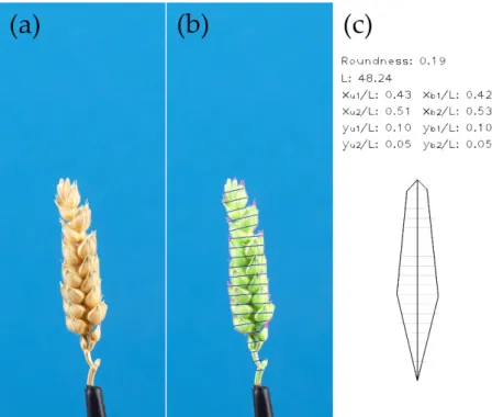
Figure S2. Stages of algorithm operation for compact spike type: (a) initial spike image; (b) the recognized spike body is highlighted with green; awn regions, with red; and sections, with blue; spike axis is denoted with red; and (c) Model of two adjacent quadrilaterals constructed based on extracted parameters.

(5)

denoted with red; and (c) Model of two adjacent quadrilaterals constructed based on extracted parameters.

(6)

(7)

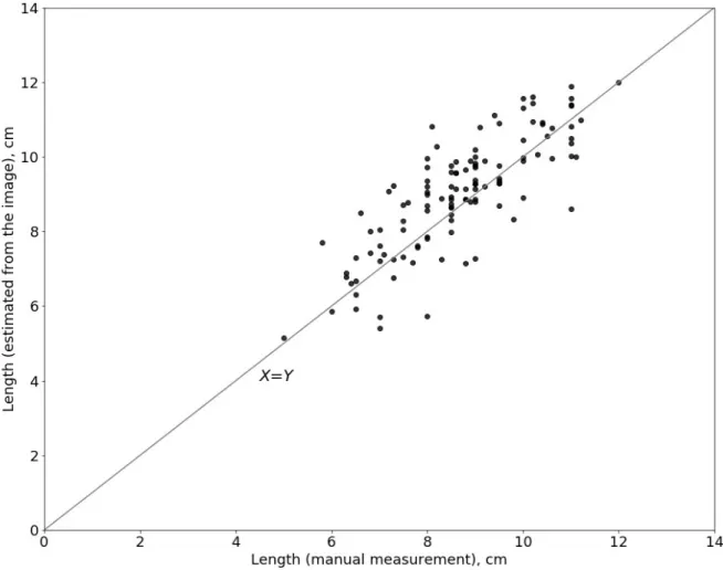
Figure S6. Scatterplot diagram for the main spike length for Triple Dirk B × KU506 F2 hybrid plants estimated manually (X axis) and from the 2D image analysis (Y axis). The solid line is Y=X line.

References

1. Kaehler, A.; Bradski, G. Learning OpenCV 3: computer vision in C++ with the OpenCV library. O'Reilly Media, Inc.2016.

2. Quintana, J.; Garcia, R.; Neumann, L.A novel method for color correction in epiluminescence microscopy.