Key-Alternating Ciphers in a Provable Setting:
Encryption Using a Small Number of Public
Permutations
Andrey Bogdanov1, Lars R. Knudsen2, Gregor Leander2, Francois-Xavier Standaert3, John Steinberger4, and Elmar Tischhauser1
1 KU Leuven and IBBT{Andrey.Bogdanov,Elmar.Tischhauser}@esat.kuleuven.be 2
Technical University of Denmark {G.Leander,Knudsen}@mat.dtu.dk 3
Universit´e catholique de Louvain, UCL Crypto Group
Tsinghua University
Abstract. This paper considers—for the first time—the concept of key-alternating ciphers in a provable security setting. Key-key-alternating ciphers can be seen as a generalization of a construction proposed by Even and Mansour in 1991. This construction builds a block cipherP X from an
n-bit permutationPand twon-bit keysk0andk1, settingP Xk0,k1(x) =
k1⊕P(x⊕k0). Here we consider a (natural) extension of the
Even-Mansour construction with t permutations P1, . . . , Pt and t+ 1 keys,
k0, . . . , kt. We demonstrate in a formal model that such a cipher is secure
in the sense that an attacker needs to make at least 22n/3 queries to the
underlying permutations to be able to distinguish the construction from random. We argue further that the bound is tight fort= 2 but there is a gap in the bounds fort >2, which is left as an open and interesting problem. Additionally, in terms of statistical attacks, we show that the distribution of Fourier coefficients for the cipher over all keys is close to ideal. Lastly, we define a practical instance of the construction witht= 2 using AES referred to as AES2. Any attack on AES2 with complexity below 285 will have to make use of AES with a fixed known key in a non-black box manner. However, we conjecture its security is 2128. Keywords: Block ciphers, provable security, Even-Mansour construc-tion, AES
1
Introduction
the wide-trail strategy [14] that lead to the design of the AES Rijndael [13]. Another line of research is the so-called provable security approach against sta-tistical attacks, that served as foundation for the block cipher MISTY [26, 27]. One can also mention the decorrelation theory [32] and the design of the ci-phers C [1] and KFC [2]. At a high level, the three main design paradigms for block ciphers are Feistel structures such as DES, Lai-Massey ciphers such as IDEA [23], and key-alternating ciphers [11, 13, 14] for which the AES Rijndael is a prominent representative. State-of-the-art block ciphers are quite well under-stood and provide security against all known attacks. Though there has recently been remarkable progress in the cryptanalysis of AES [7], these results are far from being any threat for the use of AES in practice. Thus, from a practical point of view, block ciphers in general and key-alternating ciphers in particular can be seen as a success story.
Given the degree of confidence in properly designed key-alternating ciphers on the practical side (e.g. with AES approved for the encryption of secret and top secret data in the USA), it is even more surprising that there has been no provable setting developed so far for the design of key-alternating ciphers on the theoretical side. Nobody seems to have even formulated the problem of whether the key-alternating cipher makes sense from this point of view. Clearly, given the state of the art, proving AES secure in any strict sense is out of reach. However, by modeling the round functions as fixed public randomly chosen permutations, we are able to precisely formulate and—as we shall see—prove the soundness of the key-alternating cipher design. The cipher we are dealing with is depicted in Figure 2 and detailed in Section 2.
We note the difference of our setting to that of an idealized Feistel cipher, often called the Luby-Rackoff construction [25], or to that of similar results obtained for the Lai-Massey schemes [33]. In these former works, for each key it is assumed that the function used in the Feistel (resp.Lai-Massey) construction is chosen at random. Directly adopting this model to the case of a key-alternating cipher immediately results in an ideal cipher (even for one round). At the same time, in most key-alternating ciphers including AES, the key is the only part of the design to define the cipher permutation and all round permutations are fixed for the entire cipher, not varying from key to key. In other words, working along the lines of [25] does not elucidate how to mix the key into the state. It is exactly this point we deal with in the present paper, both at a high-level, i.e. in a provable setting, as well as at lower-levels, i.e. considering statistical attacks and as a guideline for actually designing ciphers.
relatively slow diffusion in the backward direction. It is precisely these properties that facilitated the related-key cryptanalysis of the full AES-192 and AES-256, e.g. [5,6] as well as the recent biclique cryptanalysis of all three full AES versions in the classical single-key model [7]. In general, these examples emphasize a relatively weak understanding of key scheduling algorithms, compared to the design of block cipher rounds. In this context, the results of this paper can be seen as a case for simple key schedules (or even no key scheduling at all). Hence, they provide new insights into the design of block ciphers.
1.1 Related Work
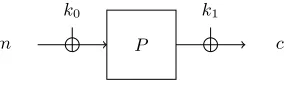
An exception from the above-mentioned lack of theoretical studies of key-alternating block ciphers is the Even-Mansour construction [15] depicted in Figure 1. This
m
k0
P
k1
c
Fig. 1.The Even-Mansour construction
construction can be seen as a one-round variant of a key-alternating cipher. Informally, Even and Mansour proved that in order to have a reasonable suc-cess probability in decrypting an (unqueried) message, an attacker has to make roughly 2n/2 queries to the permutationP. In this setting, the attacker is given oracle access toP, its inverse, and to an encryption and decryption oracle. Later, Daemen [10] showed that this bound is actually tight. He presented a differential attack on the Even-Mansour scheme that allows to successfully recover the key with a good probability, after 2n/2 evaluations of both the permutation P and the encryption oracle.
1.2 Our Contribution
Our contributions in this paper are twofold.
On the theoretical side (cf. Section 3), we provide the first treatment of the concept of key-alternating ciphers in a provable security setting. We prove below that, for anyt-round version of the cipher with randomly drawn and fixed underlying permutations,t≥2, depicted in Figure 2, an attacker needs to make at least 22n/3queries before being able to distinguish the encryption oracle from a random permutation. Here nis the block size of the cipher. Furthermore, we provide a simple attack that shows that an attacker, by making 2t+1t n queries,
leave proving this as an important open question (see also Section 7). Note that in this setup, we necessarily only consider the query complexity of an attacker, ignoring the computational complexity. It seems unlikely that an attack with a comparable computational complexity exists. Such an attack would in particular imply an attack on e.g. AES-256 with a complexity of around 2120 operations.
On the practical side, we propose to actually use the construction of Figure 2. Given our theoretical results, the merit of this approach is the following: Any attack on a key-alternating cipher with complexity below 22n/3will have to make use of the round functions in a non-black box manner.
However, and we feel that it is important to make this point explicit even though it might be obvious, the theoretical result does not carry over to any efficient instance, as one must consider the round functions as black-boxes— i.e. objects which the adversary must query to evaluate—in order to meaningfully discuss the distinguishability of the cipher from a random permutation by an information-theoretic adversary.
This fact and the fact that, as mentioned above, the theoretical bounds are likely to be lower than the computational complexity of any attack, motivates us to study the security of our proposal with respect to such statistical attacks as linear cryptanalysis (see Section 5).
To capture the difference between the single-round Even-Mansour cipher and the multiple-round key-alternating construction with respect to linear cryptanal-ysis, we study the Fourier spectrum of the ciphers. We prove that once the fixed underlying permutations are close to average (which is the case for randomly drawn permutations with high probability), the distribution of Fourier coeffi-cients for the key-alternating cipher over all keys for t ≥ 2 gets close to that over all permutations — the natural reference point for any block cipher. At the same time, we demonstrate that this is not the case for the original Even-Mansour construction with t = 1 where the Fourier coefficients almost do not change from key to key. It seems therefore unlikely that linear attacks are able to break the multiple-round key-alternating cipher witht≥2.
Finally, as the crypto community likes targets and we anticipate that having a concrete proposal is a valuable stimulation for further research, we propose an actual cipher called AES2following the 2-round version of the general construc-tion (see Secconstruc-tion 6). Here we replace the random permutaconstruc-tions by two instanti-ations of AES-128 with fixed known keys. Given the new AES instructions on recent Intel processors, AES2 performs very competitively on those platforms, with as few as 2.65 cycles per byte required in the counter mode.
We conclude with a section dedicated to open questions and further work (Section 7), discussing how to possibly improve and extend the research we consider in the paper.
2
The Construction
AES and used without being explicitly named even before that [11] in simi-lar contexts. Such a cipher consists of round functions interleaved with xoring round keys to the current state. In our idealized model, the round functions are the public, randomly chosen permutations Pi and the key consists of t+ 1 independent round-keys are ki. More precisely, let P1, . . . , Pt be permutations from{0,1}n to{0,1}n,t≥1. Letk
0, . . . , kt∈ {0,1}n be keys. The block cipher E=Ek0,...,kt :{0,1}
n→ {0,1}n we consider is defined by
E(x) =Ek0···kt(x) =Pt(. . . P2(P1(x⊕k0)⊕k1). . .)⊕kt (1)
forx∈ {0,1}n. The cipher is shown in Figure 2.
m
k0
P1
k1
P2 Pt
kt
c
Fig. 2.A key-alternating cipher
3
Indistinguishability Analysis
Putting N = 2n, we define the PRP security of E against an adversary A expecting a (t+ 1)-tuple of oracles as
AdvPRPE,N,t(A) = Pr[k0· · ·kt← {0,1}n;AEk0···kt,P1,...,Pt = 1]−Pr[AQ,P1,...,Pt= 1]
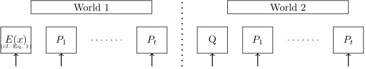
where in each experimentQ, P1, . . . , Ptare independent and uniformly sampled random permutations. Here A can make inverse queries to each of its oracles. Thus, an attacker has to tell apart two worlds, depicted below.
World 1
E(x)
(cf. Eq. 1) P1 Pt
World 2
Q P1 Pt
We note that one must consider the permutations P1, . . . , Pt as random (or pseudorandom) black-boxes—i.e. objects which the adversary must query to evaluate—in order to meaningfully discuss the distinguishability ofEk0,...,kt from a random permutation by an information-theoretic adversary.
We define
AdvPRPE,N,t(q) = max
A Adv
PRP
where the maximum is taken over all adversariesAmaking at mostqqueries. (We note the parametersnandt are elided from both of the notationsAdvPRPE (A) and AdvPRPE (q); but it should be understood thatAdvPRPE (q) is a function n andt as well as ofq.)
Our main security result is the following:
Theorem 1. Let N = 2n and let q=Nt+1t /Z for some Z ≥1. Then, for any
t≥1, and assumingq < N/100, we have
AdvPRPE,N,t(q)≤4.3q
3t
N2 + t+ 1
Zt .
For t ≥ 2 the limiting term in the above bound is 4q3t/N2, which caps q at aroundN2/3. The following corollary is more telling.
Corollary 1. Assume t≥2. Letq=N23/λ3
√
tfor someλ≥1. Then, assuming
q < N/100,
AdvPRPE,N,t(q)≤4.3
λ3 + t+ 1 (√3tλ)t.
We also note that q < N/100 as long as n ≥ 20; this condition is therefore compatible with practical parameters. We note that Corollary 1’s security of q≈N23 is optimal fort= 2 (cf. Section 3.1) and suboptimal fort >2, in which
case we conjecture a security ofq ≈Nt+1t . Closing this gap might be obtained
by a tightening of Proposition 2 below.
Theorem 1 is proved by a hybrid argument involving an intermediate game. In order to outline this hybrid argument we start by developing some new notation. Note firstly that ifE is defined as in (1) then, puttingP0=E−1, we have
P0(Pt(· · ·P1(· ⊕k0)· · ·)⊕kt) =id.
ApplyingP0−1 to both sides and then substitutingP0(·) for the input, we find
Pt(· · ·P2(P1(P0(·)⊕k0)⊕k1)· · ·)⊕kt=id. (2)
It is easy to see that, for fixedk0, . . . , kt, randomly samplingP1, . . . , Pt, defining E as in (1) and giving an adversary access to the tuple of oracles (E, P1, . . . , Pt) (and their inverses) is equivalent to sampling P0, . . . , Pt uniformly at random from all (t+ 1)-tuples of permutations satisfying (2) and giving the adversary access to (P0−1, P1, . . . , Pt) (and their inverses). Moreover, it is just a notational change to give the adversary access to (P0, P1, . . . , Pt), since the adversary is allowed inverse queries anyway (of course, the adversary is alerted to the fact that its first oracle is now P0 and notP0−1).
precisely,P0, . . . , Ptare initially set to be undefined everywhere. When the ad-versary makes a queryPi(x) orPi−1(y), the adversary definesPi at the relevant point using the following procedure, illustrated for the case of a forward query Pi(x) (the case of a backward query is analogous):
• Let P = P(P0, . . . , Pt) be the set of all (t+ 1)-tuples of permutations (P0, . . . , Pt) such that Pi extends the currently defined portion ofPi, and such that
Pt(· · ·P2(P1(P0(·)⊕k0)⊕k1)· · · ⊕kt−1)⊕kt=id. (3)
ThenO(N, t) samples uniformly at random an element (P0, . . . , Pt) fromP. The adversary setsPi(x) =Pi(x) and returns this value.
After the above, the adversary “forgets” about P0, . . . , Pt, and samples these afresh at the next query. It is clear that this lazy sampling process gives the same distribution as sampling the tuple (P0, . . . , Pt) at the start of the game. Thus, giving the adversary oracle access to O(N, t) is equivalent to giving the adversary oracle access to (E, P1, . . . , Pt), up to the cosmetic change thatE is replaced byE−1. We therefore have:
Proposition 1. WithO(N, t)defined as above, we have:
AdvPRPE,N,t(A) = Pr[k0· · ·kt← {0,1}n;AO(N,t)= 1]−Pr[AQ0,Q1,...,Qt = 1]
whereQ0, . . . , Qtare independent random permutations.
(We emphasize that k0, . . . , ktare implicit arguments toO(N, t).)
Our hybrid will be an oracle ˜O(N, t) (also takingk0, . . . , ktas implicit inputs) that uses a slightly different lazy sampling procedure to define the permutations P0, . . . , Pt. Say that a sequence of partially defined permutations is consistent if P(P0, . . . , Pt)6=∅, with P(·) defined as in the description of O(N, t) above. Initially, ˜O(N, t) also sets the permutations P0, . . . , Pt to be undefined every-where. Upon receiving (say) a forward query Pi(x), ˜O(N, t) uses the following lazy sampling procedure to answer:
• LetU ⊆ {0,1}nbe the set of valuesysuch that definingPi(x) =ymaintains the consistency ofP0, . . . , Pt, besides maintaining the fact that Pi is a per-mutation. Then ˜O(N, t) samples a valueyuniformly fromU, setsPi(x) =y, and returnsy.
Inverse queries are lazy sampled the same way. While not immediately apparent, the above lazy sampling procedure produces a slightly different distribution of outputs than the first lazy sampling procedure.
Theorem 1 is an direct consequence of Proposition 1 and of the following two propositions.
Proposition 2. Let q < N/100. WithO(N, t)andO(N, t)˜ defined as above,
Pr[k0, . . . , kt← {0,1}n;AO(N,t)= 1]−Pr[k0, . . . , kt← {0,1}n;A ˜
O(N,t)= 1]≤ 4.3q3t N2
Proposition 3. Let q=Nt+1t /Z for some Z ≥1 be such that q < N/3. With
˜
O(N, t)defined as above,
Pr[k0, . . . , kt← {0,1}n;A ˜
O(N,t)= 1]−Pr[AQ0,...,Qt = 1]≤t+ 1 Zt+1.
for every adversaryA making at mostq queries, whereQ0, . . . , Qt are
indepen-dent random permutations.
Proposition 2 is the main technical hurdle in our proof. Its proof, however, is entirely combinatorial, given that we actually show this bound holds even when A sees the keysk0, . . . , kt. The presence of keys is therefore actually irrelevant for this proposition1. We refer to Appendix A for more details.
The proof of Proposition 3, on the other hand, is fairly accessible, and also contains those ingredients that have the most “cryptographic interest”.
Proof (of Proposition 3.).We make the standard assumption that the adversary never makes a redundant query (queryingPi±1(x) twice or querying, e.g.,Pi(x) after obtainingxas an answer to a queryPi−1(y)).
We modify ˜O(N, t) to use a slightly different lazy sampling method, equiva-lent to ˜O(N, t)’s original sampling method. In this new method, we also maintain a flagbadwhich is originally set to false.
˜
O(N, t)’s new sampling method is as follows: when faced with a queryPi(x), ˜
O(N, t) samples a value y uniformly at random from the remaining range of Pi(x), that is, uniformly at random from
{0,1}n\{Pi(x0) :x0∈ {0,1}n, Pi(x0) is defined}.
˜
O(N, t) then checks if settingPi(x) =y would makeP0, . . . , Ptinconsistent; if so, it setsbad=true, and resumes its original sampling method for the rest of the game (including to answer the last query); otherwise, it setsPi(x) =y, and returnsy. Inverse queries are treated the same.
We can also define a value for thebad flag when the adversary has oracle access to the random permutations (Q0, Q1, . . . , Qt). Originally, setbad=false and select random valuesk0, . . . , kt. SetQ0, . . . , Qtto be undefined at all points, and use lazy sampling to define them by simulating the lazy sampling process for P0, . . . , Pt up until bad=true; after bad=true, simply keep lazy sampling each permutationQi while ignoringbadas well ask0, . . . , kt.
Obviously, the probabilitybadis set totrueis equal in both worlds, and the two worlds behave identically up until bad=true. Thus (a standard argument shows that) the adversary’s advantage is upper bounded by the probability that badis set totrue.
For simplicity, we upper bound the probability thatbadbecomes truewhen the adversary has oracle access toQ0, . . . , Qt. In this case, note that it is equiv-alent to set the badflag by sampling the valuesk0, . . . , kt randomly at the end
1 We note that the bound of Proposition 2 is the bottleneck of Theorem 1. A potential
of the game, and then checking whether these values are inconsistent with the partially defined permutationsQ0, . . . , Qt. (To recall,k0, . . . , ktare inconsistent withQ0, . . . , Qtif there exist no permutationsQ0, . . . , Qtsuch that
Qt(· · ·Q2(Q1(Q0(·)⊕k0)⊕k1)· · · ⊕kt−1)⊕kt=id.)
Given the partially defined permutations Q0, . . . , Qt and values k0, . . . , kt a contradictory path is a sequence of values (x0, y0), . . . ,(xt, yt) such that (i) Qi(xi) =yi for all iand (ii) |{i:yi⊕xi+1 =ki,0≤i≤t}|=t, where we put xt+1=x0. Because q < N/3, Lemma 3 of Section A implies2 thatQ0, . . . , Qtis consistent withk0, . . . , ktif and only if there exists no contradictory path. Since eachQi contains at mostqdefined input-output pairs (xi, yi) at the end of the game, there are at most qt+1 possible different sequences ((x0, y0), . . . ,(xt, yt)) such that Q(xi) =yi for 0≤i≤t. For each of these sequences, the probability that the random selection of k0, . . . , kt creates a contradictory path is upper bounded by (t+ 1)N−t, since the conditionk
i =yi⊕xi+1 must be satisfied for all but one value ofi, 0≤i≤t, and we can union bound over this value of i. Hence, by a union bound over the (at most) qt+1 possible different sequences, the probability thatbadis set totrueis at most (t+1)Nqtt+1 =
t+1
Zt as desired.
3.1 An upper bound
For any number of roundst, there is an (non-adaptive) attack with a query com-plexity of roughlyt2t+1t n, thus meeting the bound on the query complexity for
t= 2. Note that this is not an attack in the practical sense, as the computational cost is higher than brute force. The idea of this attack is to actually construct (with high probability) a contradictory path for each possible key.
1. Make 2t+1t nqueries to Eand each of the oraclesP1 toPt. Denote the set of
queries toPi byPi and queries toEk byM. 2. For each key candidate (k0, k1, . . . , kt) do:
(a) Find all sequences of values (x1, . . . , xt−1) such thatx1 ∈ Mand xi⊕ ki−1∈ Pi, ∀1≤i≤t andPi(xi⊕ki−1) =xi+1, ∀1≤i≤t−1.
(b) Check ifPt(xt⊕kt−1)⊕kt=E(x1) for all these sequences. (c) If so, assume (k0, k1, . . . , kt) is the correct value of the key; (d) otherwise, it is certainly the wrong value of the key.
To get a better reduction on key-candidates, a bit more thant2t+1t n queries are
sufficient.
2 More precisely, Lemma 3 is applied by setting the edges of the matchingM
ito be all pairs (xi, yi⊕ki) such thatQi(xi) is defined; that isMiencodes the permutation
4
Attacks
The bounds proved earlier are information-theoretic bounds which take into account only the number of queries of the random permutations made by an adversary. Of equal interest are attacks which take the computational complexity into account. In this section we consider only attacks in the single key-model. Note that, in the case where all round-keys are independent, related-key attacks exist trivially. However, the situation might be very different in the case where all round-keys are identical, see Section 7 for further discussion on this point.
4.1 Daemen’s attack for t= 1
For the original Even-Mansour construction (in our setting, this corresponds to t = 1), a differential attack has been published by Daemen [10] meeting the lower bound of 2n/2 evaluations of P proven by Even and Mansour. It can be described as follows:
1. Choose s plaintext pairs (mi, m∗i), 1 ≤ i ≤ s, with mi⊕m∗i =∆ for any nonzero constant∆.
2. Get the encryptions (ci, c∗i) of thespairs. 3. For 2n/svaluesv:
(a) Compute w0:=P(v)⊕P(v⊕∆).
(b) Ifw0=ci⊕c∗i for somei: Outputk0:=v⊕m1andk1:=c1⊕P(m1⊕k0) and stop.
For a random permutationP, only very few values ofv are expected to satisfy P(v) +P(v+∆) = ci ⊕c∗i. The wrong candidates can be easily filtered in step (3b) by testing them on a few additional encryptions. After encrypting s plaintext pairs, one has to perform about 2·2n/sevaluations ofP. The expression 2(s+ 2n/s) is minimal for s = 2n/2. In this case, the time complexity is 2n/2 with a storage requirement of 2n/2 plaintext pairs.
4.2 A meet in the middle attack
There is a meet in the middle attack on the t-permutation construction which finds the keys in time and space 2tn/2fort >1. This is a straight-forward attack given here for the caset= 2:
1. From a pair of messages (m1, m2), compute and save in a sorted table,T, the valuesP(m1⊕k)⊕P(m2⊕k) for all possible 2n values ofk.
2. Get the encryptions c1 andc2 ofm1 respectivelym2.
3. For all 2npossible values ofk0computeQ−1(c1⊕k0)⊕Q−1(c2⊕k0) and look for a match inT.
5
Statistical Properties
A fundamental cryptographic property of a block cipher is its Fourier spectrum that completely defines the cipher via the Fourier transform and whose distri-bution is closely related to the resistance against linear cryptanalysis [9].
To support security claims, block cipher designs usually come with arguments why these Fourier coefficients cannot take values exploitable by an attacker. In most cases, however, formal proofs of these properties appear technically infeasible and designers limit themselves to demonstrating upper bounds on trail probabilities, that can be seen as summands to obtain the actual Fourier coefficients. This solution is usually denoted as the practical security approach for statistical cryptanalysis. Such an approach does not allow an accurate estimation of the data complexity of statistical attacks, that typically depends on numerous trails [24, 28].
As opposed to that, we analyze the construction of key alternating cipher following a provable security approach, by directly investigating its Fourier co-efficients. In addition, we provide a more informative analysis than for standard block ciphers, as we study the distribution of the Fourier coefficients for the cipher over all keys, rather than bounding the mean value of this distribution. This is made possible by the use of fixed public permutations in our construction. More precisely, in a key-alternating cipher usingt≥2 fixed public permutations, we study the distribution of the Fourier coefficients over all cipher keys. If these permutations are close to the average over all permutations, we show that this distribution turns out to be very close to that over all permutations, suggesting that the t-round key-alternating construction is theoretically sound from this perspective. This implies that it behaves well with respect to linear cryptanaly-sis.
On the contrary, the distribution of Fourier coefficients for a fixed point in the Fourier spectrum is nearly degenerated for the key-alternating cipher with t = 1 (the Even-Mansour cipher). This emphasizes the constructive effect of having 2 and more rounds in the key-alternating cipher.
5.1 Fourier coefficients over all permutations
Here we recall the definitions of Fourier coefficients and Fourier spectrum as well as the distribution of Fourier coefficients over all permutations. We also introduce some notations we will be using throughout the section.
Notations. The canonical scalar product of two vectorsa, b∈ {0,1}nis denoted by aTb. We denote the normal distribution with mean µ and variance σ2 as
N(µ, σ2). ByX ∼
v D, we denote a random variableX following a distribution
Fourier coefficients and Fourier spectrum. For a permutationP :{0,1}n →
{0,1}n, itsFourier coefficient at point (α, β) is defined as
Wα,βP def= X x∈{0,1}n
(−1)αTx+βTP(x).
The collection of Fourier coefficients at all points (α, β) ∈ {0,1}n× {0,1}n is called theFourier spectrum of P. For a block cipher F, we denote the Fourier coefficient at point (α, β) asWα,βF [K] to emphasize its dependency on keyK. If F is thet-round key-alternating cipher, this is denoted byWP1,...,Pt
α,β [K]. The following characterisation for the distribution of Fourier coefficients in a Boolean permutation has been proven.
Fact 1 ([12, Corollary 4.3, Lemma 4.6]). When n≥5, the distribution of the Fourier coefficientWαP
0,β0 withα0, β06= 0over alln-bit permutations can be
approximated by the following distribution up to continuity correction:
WαP0,β0 ∼P N(0,2n). (4)
The distribution of Fact 1 is the reference point throughout the section: A block cipher cannot have a better distribution of Fourier coefficients than that close to Fact 1.
5.2 Fourier coefficients in the single-round Even-Mansour cipher
Let F be the basic single-round Even-Mansour cipher, that is, a fixed public permutation P surrounded by two additions with keys k0 and k1, respectively (see Figure 1). IfWP
β0,β1 is the Fourier coefficient for the underlying permutation
P at point (β0, β1), then the Fourier coefficient for the cipher at this point is
WβF0,β1= (−1)
βT
0k0⊕β
T
1k1WP
β0,β1.
Now consider the distribution ofWβF
0,β1 withβ06= 0,β16= 0 taken over all keys
(k0, k1). Its support contains exactly two points:WβP0,β1 and−W
P
β0,β1. Thus, the
value ofWF
β0,β1 almost does not vary from key to key. This is crucially different
from the reference point – the distribution over all permutations of Fact 1.
5.3 Fourier coefficients in the t-round key-alternating cipher
Now we state the main result of this section. The proof is given in Appendix B.
Theorem 2. Fix a point(β0, βt)withβ0, βt6= 0in the Fourier spectrum of the t-round key-alternating n-bit block cipher with round permutations P1, . . . , Pt
fort≥2 and sufficiently highn. Then the distribution of the Fourier coefficient
WP1,...,Pt
β0,βt at this point over all keysK is approximated by:
WP1,...,Pt
β0,βt [K]∼KN(0,(1 +ε)
2n−1 2n
t−1
assuming that the distributions over points of the Fourier spectra of the permu-tations Pi,1≤i≤t, have variances satisfying
Var (βi−1,βi)
h
WPi βi−1,βi
i
≥2n/2, (6)
and that for any given key K, the signs of the Fourier coefficients behave in-dependently for different points. The deviation of the permutationsPi from the mean over all permutationsQi is quantified by factor (1 +ε):
P
(β1,...,βt−1)
WP1
β0,β1· · ·W
Pt βt−1,βt
2
= (1 +ε)·EQ1,...,Qt
P
(β1,...,βt−1)
WQ1
β0,β1· · ·W
Qt βt−1,βt
2
.
(7)
Interestingly, the latter deviation ε from the mean in (7) is small for most choices of the Pi. For instance, in case t = 2, it can be shown that over all permutations, mean and variance of each summand in (7) are 22n and 24n+2, respectively. The whole sum then approximately follows a normal distribution
N(23n−22n,25n+2−24n+2). This means that forrandomly drawn permutations
P1, P2, the sumPβ1
WP1
β0,β1W
P2
β1,β2 2
will be withindstandard deviations from
its mean with probability erf d/√2. Notably, this implies Pr(|ε| ≤2−n/2+3)≈
0.9999, i.e.|ε|only very rarely exceeds 2−n/2+3.
Theorem 2 gives the distribution over all keys of the Fourier coefficient WP1,...,Pt
β0,βt individually for each nontrivial point (β0, βt). Appropriate choices for thePi should have distributions close to N(0,2n) for each nontrivial point, not only for some of them. Conversely, the distribution of the Fourier coefficient at the (trivial) point (β0,0) differs from (5) for any choice of the Pi, since it is constant over the keys.
Note also that the result of Theorem 2 does not require the underlying per-mutations to be different. Moreover, it does not require the perper-mutationsPi to be randomly drawn from the set of all permutations, but holds for any fixed choice of permutations satisfying (6). To obtain a distribution close to ideal, however, the set of underlying permutations has to ensure a small deviation ε in (7). As argued above, drawing the underlying permutations at random from the set of all permutations is highly likely to result in a very small deviation ε from the average.
Summarising, the results of Theorem 2 suggest that once the small number oft≥2 underlying permutations are carefully chosen and fixed, thet-round key-alternating cipher for each secret key is likely to be statistically sound which rules out some crucial cryptanalytic distinguishers. More precisely, the distributions of the Fourier coefficients for the t-round key-alternating cipher over all keys become close to those over all permutations.
one fixes all keys k1 up to kt−1. For any point (β0, β1) the value of W P1,...,Pt β0,βt takes on only two possible values - over all possible sub-keysk0, kt. However, it seems unlikely that this can be used in an attack.
6
Practical constructions
In this section, we discuss possible practical realisations of the t-round key-alternating cipher.
A natural approach to building a practical cipher following thet-permutation construction is to base thetfixed permutations on a block cipher by fixing some keys. Witht= 1, this corresponds to the original Even-Mansour construction, so the security level is limited to 2n/2operations withndenoting the cipher’s block length. With a 128-bit block cipher such as the AES, we therefore only obtain a security level of 264 in terms of computational complexity, so it is advisable to choose t >1.
In the following we describe a sample construction with t = 2, that is, we consider the 2-round key alternating construction with permutationsP1 andP2 and the keysk0, k1, k2.
6.1 AES2: a block cipher proposal based on AES
The construction is defined by fixing two randomly chosen 128-bit AES-128 keys, which specifies the permutationsP1andP2. The key is comprised by three independently chosen 128-bit secret keysk0, k1, k2.
Let AES[k] denote the (10-round) AES-128 algorithm with the 128-bit key k and the 128-bit quantitiesπ1, π2be defined based on the first 256 bits of the binary digit expansion ofπ= 3.1415. . .:
π1:=0x243f6a8885a308d313198a2e03707344 and π2:=0xa4093822299f31d0082efa98ec4e6c89.
Then we denote the resulting 2-permutation construction by AES2[k0, k1, k2]. Its action on the 128-bit plaintextmis defined as:
AES2[k0, k1, k2](m) := AES[π2](AES[π1](m⊕k0)⊕k1)⊕k2. (8)
Performance. AES2can be implemented very efficiently in software on general-purpose processors. The two AES keys π1 and π2 are fixed and, therefore, the round keys for the two AES transformations can be precomputed, so there is no need to implement the key scheduling algorithm of AES. This ensures high key agility of AES2.
On the Westmere architecture generation of Intel general-purpose proces-sors, AES2 can be implemented using the AES-NI instruction set [18]. As the AES round instructions are pipelined, we fully utilise the pipeline by processing four independent plaintext blocks in parallel implementing the basic electronic codebook mode (ECB) and counter mode (CTR). The performance of these im-plementations on recent processors is demonstrated and compared to two con-ventional implementations of AES-128 (i.e. without AES-NI instructions) – the bitsliced implementation of [20] and the OpenSSL 1.0.0e implementation based on lookup tables. All numbers are given in cycles per byte (cpb).
Intel Xeon X5670 Intel Core i7 640M
2.93 GHz, 12 MB L3 cache 2.8 GHz, 4 MB L3 cache
AES2, AES-NI, ECB 2.54 cpb 2.69 cpb
AES2, AES-NI, CTR 2.65 cpb 2.76 cpb
AES-128, AES-NI, ECB 1.18 cpb 1.25 cpb
AES-128, AES-NI, CTR 1.32 cpb 1.36 cpb
AES-128, bitsliced, CTR 7.08 cpb 7.84 cpb
AES-128, OpenSSL, CTR 15.73 cpb 16.76 cpb
It turns out that on both platforms, the performance of AES2is almost equal to half that of AES, indicating that the overhead is very low. Compared to the best implementations of the AES which are in widespread use now on standard platforms, AES2provides a performance improvement of almost factor three and higher with the AES-NI instruction set.
7
Conclusion, Open Problems and Future Work
In this paper we gave the first formal treatment of the key-alternating cipher in a provable setting. For two or more rounds an attacker needs to query the oracles at least 22n/3 times for having a reasonable success probability. Furthermore, we studied the security of the construction with respect to statistical attacks, arguing that even fort= 2 linear attacks do not seem to be applicable. Finally we gave a concrete proposal mimicking the construction for t = 2. There are several lines of future work and open problems we like to mention.
independent. For aesthetical reasons, but also from a practical point of view (see below) it would be nice to prove bounds for the case that all round keys are identical.
On the practical side, mainly for efficiency reasons but also due to resistance against related-key attacks, several variants for t= 2 are worth studying. First of all, since the security level is at most 2n, due to the meet in the middle attack, one could be tempted to derive threen-bit keys k0, k1,and k2 from one n-bit word. The simplest case here is to have all three keys identical. TakingP andQdifferent, we are not aware of any attack with computational complexity below 2n. Furthermore, it seems reasonable to assume that such a construction provides some security against certain types of related-key attacks as well. The best attacks we are aware of in such a setting has birthday complexity 2n/2. See Appendix C for the details.
Eventually, it is an interesting open problem to determine whether the results in this work can be used as directions for alternative block cipher designs, e.g. with minimum key scheduling algorithms. As a typical example, one could con-sider the possibility to generate public permutations from a variant of the AES, where the round keys would be replaced with simple constants. In general, such an approach could lead to efficient lightweight designs. Interestingly, it is also the direction taken, to a certain extent, by the recently proposed block cipher LED [19]. In its 64-bit version, this cipher just iterates blocks made of 4 rounds and the addition of the master key.
Another tempting way, in order to increase efficiency, is to chooseQ =P. Similarly, it may be advantageous to have Q = P−1, which has the further advantage that the decryption and encryption operations are similar, except for using the keys in reverse order. However, withQ=P−1there is an attack which finds the value of k0⊕k2 using 2n/2 queries and similar time. After k0⊕k2 is known the cipher is easily distinguishable from a random permutation. Also, withQ=P but now assuming that k0⊕k2 is known, one finds the secret keys using 2n/2 queries and similar time.
References
1. Thomas Baign`eres and Matthieu Finiasz. Dial C for Cipher. Selected Areas in Cryptography, LNCS 4356, pp. 76–95, Springer-Verlag, 2006.
2. Thomas Baign`eres and Matthieu Finiasz. KFC - The Krazy Feistel Cipher. ASI-ACRYPT 2006, LNCS 4284, pp. 380–395, Springer-Verlag, 2006.
3. Paulo S.L.M. Barreto and Vincent Rijmen. The KHAZAD Legacy-Level Block Cipher. First open NESSIE Workshop, 15 pages, Leuven, Belgium, November 2000. 4. G. Bertoni, J. Daemen, M. Peeters, and G. Van Assche. Keccak sponge function
family main document. Submission to NIST (Round 2), 2009.
5. Alex Biryukov, Orr Dunkelman, Nathan Keller, Dmitry Khovratovich and Adi Shamir. Key Recovery Attacks of Practical Complexity on AES-256 Variants with up to 10 Rounds. EUROCRYPT 2010, LNCS 6110, pp. 299–319, Springer-Verlag, 2010.
6. Alex Biryukov and Dmitry Khovratovich. Related-Key Cryptanalysis of the Full AES-192 and AES-256. ASIACRYPT 2009, LNCS 5912, pp. 1–18, Springer-Verlag, 2009.
7. Andrey Bogdanov, Dmitry Khovratovich and Christian Rechberger. Biclique Cryptanalysis of the Full AES. ASIACRYPT 2011, LNCS 7073, pp. 344–371, Springer-Verlag, 2011.
8. Andrey Bogdanov, Lars R. Knudsen, Gregor Leander, Christof Paar, Axel Poschmann, Matthew J. B. Robshaw, Yannick Seurin and C. Vikkelsoe: PRESENT: An Ultra-Lightweight Block Cipher. CHES 2007, LNCS 4727, pp. 450– 466, Springer-Verlag, 2007.
9. Florent Chabaud and Serge Vaudenay. Links between differential and linear crypt-analysis. EUROCRYPT 94, LNCS 950, pp. 356–365, Springer-Verlag, 1995. 10. Joan Daemen. Limitations of the Even-Mansour Construction. ASIACRYPT 1991,
LNCS 739, pp. 495–498, Springer-Verlag, 1991.
11. Joan Daemen, Rene Govaerts and Joos Vandewalle. Correlation matrices. FSE 1994, LNCS 1008, pp. 275–285, Springer-Verlag, 1995.
12. Joan Daemen and Vincent Rijmen. Probability distributions of correlations and differentials in block ciphers. Journal on Mathematical Cryptology 1(3), pp. 221– 242, 2007.
13. Joan Daemen and Vincent Rijmen. The Design of Rijndael. Springer-Verlag, 2002. 14. Joan Daemen and Vincent Rijmen. The Wide Trail Design Strategy. IMA Int.
Conf., LNCS 2260, pp. 222–238, Springer-Verlag, 2001.
15. Shimon Even and Yishay Mansour. A Construction of a Cipher from a Single Pseudorandom Permutation. J. Cryptology, vol. 10, num. 3, pp. 151–162, 1997. 16. Shimon Even and Yishay Mansour. A Construction of a Cipher From a Single
Pseu-dorandom Permutation. ASIACRYPT 1991, LNCS 739, pp. 210–224, Springer-Verlag, 1993.
17. FIPS PUB 46-3: DATA ENCRYPTION STANDARD (DES). 1999.
18. Shay Gueron. Intel Mobility Group, Israel Development Center, Israel: In-tel Advanced Encryption Standard (AES) Instructions Set, 2010. Available at http://software.intel.com/file/24917.
19. Jian Guo, Thomas Peyrin, Axel Poschmann and Matt Robshaw: The LED Block Cipher. CHES 2011, LNCS 6917, pp. 326–341, Spinger-Verlag, 2011.
21. Liam Keliher, Henk Meijer and Stafford E. Tavares. Improving the Upper Bound on the Maximum Average Linear Hull Probability for Rijndael. Selected Areas in Cryptography, LNCS 2259, pp. 112–128, Springer-Verlag, 2001.
22. Lars R. Knudsen. Practically Secure Feistel Ciphers. FSE 1993, LNCS 809, pp. 211– 221, Springer-Verlag, 1991.
23. Xuejia Lai and James L. Massey. A Proposal for a New Block Encryption Standard. EUROCRYPT 1990, LNCS 473, pp. 389–404, Springer-Verlag, 1990.
24. Xuejia Lai and James L. Massey. Markov Ciphers and Differentail Cryptanalysis. EUROCRYPT 1991, LNCS 547, pp. 17–38, Springer-Verlage, 1991.
25. Michael Luby and Charles Rackoff. How to Construct Pseudorandom Permutations from Pseudorandom Functions. SIAM J. Comput., vol. 17, num. 2, pp. 373–386, 1988.
26. Mitsuru Matsui. New Block Encryption Algorithm MISTY. FSE 1997, LNCS 1267, pp. 54–68, Springer-Verlag, 1997.
27. Mitsuru Matsui. New Structure of Block Ciphers with Provable Security against Differential and Linear Cryptanalysis. FSE 1996, LNCS 1039, pp. 205–218, Springer-Verlag, 1996.
28. Kaisa Nyberg. Linear Approximation of Block Ciphers. EUROCRYPT 1994, LNCS 950, pp. 439–444, Springer-Verlag, 1994.
29. Luke O’Connor. Properties of Linear Approximation Tables. FSE 1994, LNCS 1008, pp. 131–136, Springer-Verlag, 1995.
30. Vincent Rijmen, Joan Daemen, Bart Preneel, Antoon Bosselaers and Erik De Win. The Cipher SHARK. FSE 1996, LNCS 1039, pp. 99–111, Springer-Verlag, 1996. 31. Aris Spanos. Probability Theory and Statistical Inference: Econometric Modeling
with Observational Data. Cambridge University Press, 1999.
32. Serge Vaudenay. Decorrelation: A Theory for Block Cipher Security. J. Cryptology, vol. 16, num. 14, pp. 249–286, 2003.
33. Serge Vaudenay. On the Lai-Massey Scheme. ASIACRYPT 1999, LNCS 1716, pp. 8–19, Springer-Verlag, 1999.
A
Proof of Proposition 2
In this section we provide a proof of Proposition 2, which constitutes the most technical part of our paper. The argument is structured as follows: Firstly, we allow the adversary A to see the values k0, . . . , kt (in fact, we even allow A to choose these values); obviously, such an adversary can only perform better than an adversary without knowledge ofk0, . . . , kt. Secondly, we argue that the ki’s can be set to 0n without any loss in advantage. The problem then reduces to upper bounding the adversary’s advantage at distinguishing two different methods of lazy sampling permutationsP0, . . . , Pt such that
Pt(· · ·P2(P1(·))· · ·) =id.
setting, the sample distinguishability game lets the adversary “set up” each of its queries as it wants; namely, it can partially define the permutationsP0, . . . , Pton at mostq points each (subject to the consistency constraint), and then request its oracle—which is either O(N, t) or ˜O(N, t)—to answer a query of its choice, for that choice ofP0, . . . , Pt; at its next query, the adversay can set upP0, . . . , Pt again from scratch, and so on. Clearly such an adversary with “set-up power” has advantage at least that of a standard adversary. We then combine the statistical distance bound for a single query (Lemma 2 below) with a simple lemma relating sampling distinguishability to single-sample statistical distance (Lemma 1 below) to obtain the final result (restated as Lemma 5 below, that is equivalent to Proposition 2).
Define
AdvON,tO˜(A) = Pr[A→k0, . . . , kt;AO(N,t)= 1]−Pr[A→k0, . . . , kt;A ˜
O(N,t)= 1]
and
AdvON,tO˜;0n(A) = Pr[k0=· · ·=kt= 0n;AO(N,t)= 1]−Pr[k0=· · ·=kt= 0n;A ˜
O(N,t)= 1].
Obviously, it suffices to show that AdvON,tO˜(A) ≤ 4.3q3t/N2 for all A making at most q < N/100 queries in order to prove Proposition 2. (Indeed A is free to choose k0, . . . , kt randomly and then forget about these values.) Our first proposition shows that, in fact, it is sufficient to upper boundAdvON,tO˜;0n(·).
Proposition 4. For everyq-query adversaryAthere exists aq-query adversary
A0 such that
AdvON,tO˜;0n(A0) =AdvON,tO˜(A).
Proof. A0 simulates A; letk0, . . . , kt be the keys chosen byA. WhenA makes a query Pi(x), A0 queries Pi(x) and returns Pi(x)⊕ki to A; when A queries Pi−1(x), A0 queries Pi−1(x⊕ki). It is easy to check that when A0’s oracle is O(N, t) (resp.O(N, t)), then˜ A0 providesAwith a perfect simulation ofO(N, t) (resp.O(N, t)) on keys˜ k0, . . . , kt. It follows thatA0’s advantage is exactlyA’s.
The rest of our effort focuses on upper boundingAdvON,tO˜;0n(A) for aq-query
ad-versaryA; namely, by Proposition 4, it is sufficient to show thatAdvON,tO˜;0n(A)< 4.3q3t/N2 when q < N/100. The latter upper bound is finally established in Corollary 2 below.
We now abstract the problem of distinguishing the oraclesO(N, t), ˜O(N, t) into a more general type of game (that is also more generous to the adversary). This game is the “sample distinguishability” game referred to above.
taken independently of previous samples; in particular, if the adversary queries the sameXα twice, then Xα is sampled twice independently. The adversary is adaptive, and can query its oracles in any order it wishes.
We next define the notion of (adaptive) sample distinguishability.
Definition 1. Let (Xα, Yα)α∈B denote a family of pairs of random variables
indexed by a finite set B, where each random variable takes values in the same finite rangeS. We define
Advsamp(X −dist
α,Yα)α∈B(A) = Pr[A
(Xα)α∈B= 1]−Pr[A(Yα)α∈B = 1]
with the probabilities being taken over the randomness of the distributions and over the adversary’s coins, if any. We also define
Advsamp(X −dist
α,Yα)α∈B(q) = maxA Adv samp−dist (Xα,Yα)α∈B(A)
where the maximum is taken over all adversariesA making at mostqqueries.
We note that non-adaptive sample distinguishability—in which case the adver-sary must announce its sequence of queries (α1, . . . , αq) before receiving any answers—reduces to upper bounding the maximum statistical distance of the form
∆((Xαi)qi=1,(Yαi)qi=1)
where (Xαi) q
i=1 is the product distribution3 (Xα1, . . . , Xαq) and likewise for (Yαi)qi=1, and with this maximum being taken over all possible sequences (α1, . . . , αq). Since all samples are taken independently (in the adaptive as well as in the non-adaptive game), it might intuitively seem that adapativity doesn’t help, but, surprisingly, it does. (An example appears at the end of this section.)
Lemma 1. Let (Xα, Yα)α∈B be a set of pairs of random variables indexed by
the finite set B. Then
Advsamp(X −dist
α,Yα)α∈B(q)≤q·maxα∈B∆(Xα, Yα).
Proof. We use a coupling argument. For eachα∈B, let ( ˜Xα,Y˜α) be a maximal coupling ofXαandYα; this means ˜Xαand ˜Yαare defined on the same probability space, such that
Pr[ ˜Xα6= ˜Yα] =∆(Xα, Yα)
and such that ˜Xαis equidistributed toXαand ˜Yαis equidistributed toYα. (That such distributions ˜Xα, ˜Yαexist is a standard fact.) When we sample ˜Xαwe thus “automatically” sample ˜Yα, and vice-versa. When an adversaryAinteracts with oracle ( ˜Xα)α∈B, letbadbe the event that, for one of the queriesαasked byA,
˜
Xα6= ˜Yα(note that only ˜Xαis returned toA). We likewise definebadwhen the
3
An r.v.X of the formX= (X1, . . . , Xq) is aproduct distributionwhen theXi’s are
adversary interacts with oracle ( ˜Yα)α∈B. Note that as long asbad=false, the two oracles are equidistributed. (Indeed, the entity performing the queries is “doing the same thing” in either world: namely, sampling the required pair ( ˜Xα,Y˜α) and returning the common value of this pair.) The adversary’s advantage is at most the probability of settingbad=truewhich, by a union over theqqueries, is at most
q·max
α Pr[ ˜Xα6= ˜Yα] =q·maxα ∆(Xα, Yα).
Note: We believe Lemma 1 is far from tight. Moreover, it currently constitutes the main “bottleneck” in our security bound. One could improve Lemma 1 by showing, for example, that the advantage of an adaptive sample distinguisha-bility adversary is upper bounded by a constant (e.g., 2) times the advantage of a non-adaptive adversary, but we do not know of such a bound. See also the example relating adaptivity to non-adaptivity at the end of this section.
To state our main technical result we need to define the family of pairs (Xα, Yα)a∈B that we are interested in applying Lemma 1 to. Parameters for this family will be N,qandt. Recall that upper boundingAdvON,tO˜;0n(A) for aq-query adversaryA means upper boundingA’s distinguishing advantage between two different lazy sampling methods for a sequence of permutationsP0, . . . , Pt such that
Pt(· · ·P1(P0(·))· · ·) =id. (9)
In the following, we model the (partially defined) permutations by their associ-ated (partial) matchings. That is, a partially defined permutation on {0,1}n is defined by a matching with left vertex set {0,1}n and right vertex set{0,1}n, in the natural way. Composing sevaral permutations corresponds to gluing the associated matchings side by side.
LetV0, . . . , Vt, Vt+1 be sets of vertices with|Vi|=N, and where we identify Vt+1 withV0 (i.e.,Vt+1 andV0are two different names for the same set).
A sequence of matchingsM = (M0, . . . , Mt+1) whereMiis a perfect match-ing betweenViandVi+1is calledcircularif every path starting at a vertexv∈V0 following the edges inM0, . . . , Mtends at the same vertexv∈Vt+1=V0. Thus, circularity is the matching equivalent of (9).
Given a sequence M = (M0, . . . , Mt) where each Mi is a partial matching betweenVi andVi+1, we let
M(M)
be the set of all circular sequences M extendingM, i.e. the set of all sequences M = (M0, . . . , Mt) such that Mi extends Mi for each i and such that M is circular. We sayM isconsistent ifM(M)6=∅. (This fits our previous definition of consistency, restricted to the casek0=. . .=kt= 0n.)
Let aq-configuration be a pair (v0, M) such that (i)M = (M0, . . . , Mt) is a consistent sequence of partial matchings such that|Mi| ≤qfor alli, (ii)v0∈V0 is nonadjacent to M0. Our index setB for the family of pairs (Xα, Yα)α∈B will be exactly the set of allq-configurations. That is,
We now describe, for a givenα= (v0, M)∈B, the distributionsXα andYα. Let α = (v0, M) be a q-configuration, M = (M0, . . . , Mt). For any vertex u∈ V1 nonadjacent to M0, we write M ∪ {(v0, u)} for the sequence of partial matchings (M0∪ {(v0, u)}, M1, . . . , Mt). LetU⊆V1be the set of verticesusuch that M∪ {(v0, u)} is consistent. We define
Pr[Xα=u] := M(M ∪ {(v0, u)})
M(M) .
We note that Xα is a probability distribution on U, and that Xα is equidis-tributed to O(N, t) queried at P0(v0) with keys k0 = . . . = kt = 0n and with P0, . . . , Pt defined such that Pi(x) =y ⇐⇒ (x, y)∈ Mi. As for Yα, it is sim-ply the uniform distribution onU. ThusYαis equidistributed to ˜O(N, t) under the same correspondence. (Note the restriction to queries of the form P0(·) is without loss of generality, since the adversary can “set up” the matchings as its wants in the sample distinguishability game.)
The crux of our proof is the following lemma:
Lemma 2. Let q < N/100 and let t ≥ 1. Then for any q-configuration α = (v0, M), we have
∆(Xα, Yα)≤ 2qρ
N−2q.
whereρ= 2.05qt/N, with Xα andYα defined as above.
We need two more small results before giving the proof of Lemma 2. For a sequence of partial matchings M = (M0, . . . , Mt), a path of length t+ 1 us-ing edges from the partial matchus-ings M0, . . . , Mt (possibly “wrapping around” throughV0=Vt+1) iscontradictory if it containst+ 2 vertices (i.e., if it is not a cycle—this is also a restatement of our previous definition of a contradictory path, restricted to the case where theki’s are 0n). Obviously, if a partial match-ing contains a contradictory path it cannot be consistent. The next lemma gives a partial converse.
Lemma 3. Letq≤N/3. Then a partial sequence of matchingsM = (M0, . . . , Mt)
where each Mi has at mostq edges each is consistent if and only if it contains no contradictory path.
Proof. We show thatM can be extended to a circular sequence of perfect match-ingsM. The extension follows three steps: (i) for each edge inM0, if such an edge is not already in a path of length t+ 1, then we complete a non-contradictory path of lengtht+1 containing that edge; (ii) we arbitrarily extend the matchings M1, . . . , Mtto perfect matchingsM1, . . . , Mt; (iii) we complete the matchingM0 to a perfect matchingM0 in the unique way that will makeM = (M0, . . . , Mt) circular.
Steps (ii) and (iii) can obviously carried out if step (i) succeeds, so it remains to prove that step (i) is possible.
no edges (note that to start with, there are at leastN/3 free nodes in eachVi). Let
(v`, v`+1, . . . , vt, vt+1=v0, v1, . . . , vk)
be the maximal path containing (v0, v1), where vi ∈ Vi, where` ≤ t+ 1 and k≥1. By assumption that there are no contradictory paths, k < `. Ifk=`−1 then we can simply connectvkandv`by an edge. Otherwise, as long as there are free nodes left in each of the layers Vk+1, . . . , V`−1, we can use these to connect vk tov` by a path. However, we start with at leastN/3 free nodes in each layer, and we have only at mostN/3 paths to create (one for each ofM0). Hence such free nodes will always exist.
The following is an elementary observation that trusting readers can take for granted.
Lemma 4. Let a setU be the disjoint union of setsR,T, and letρ∈[0,12]. Let
Y be the uniform distribution overU and let X be a random variable such that
Pr[X =u1] = Pr[X =u2] for allu1, u2∈R and such that
Pr[X=u1]∈[(1−ρ) Pr[X=u2],(1−ρ)−1Pr[X =u2]] (10)
for allu1, u2∈U. Then
∆(X, Y)≤ 2ρ|T| |U| .
Proof. We start by noting that since there must exist some u1 ∈ U such that Pr[X =u1]≤1/|U|, and also someu2 ∈U such that Pr[X =u2]≥1/|U|, the second condition implies that
Pr[X =s]∈[(1−ρ)/|U|,(1−ρ)−1/|U|]
for all s ∈ U. We also note thatρ ∈ [0,12] implies (1−ρ)−1 ≤ 1 + 2ρ. Since
|Pr[X = s]−Pr[Y = s]| ≤ 2ρ/|U| for all s, the lemma obviously holds when
|T|=|U|. We can therefore assumeR6=∅.
Letp be the probability Pr[X =u] for some u∈ R (where by assumption this probability does not depend on the choice ofu∈R). We consider two cases according to whetherp≥1/|U|orp≤1/|U|. Assume first thatp≤1/|U|. Then Pr[X =s]≤Pr[Y =s] for alls∈R, so
∆(X, Y) = max S⊆U
X
s∈S
Pr[X =s]−Pr[Y =s]
= max
S⊆TPr[X =s]−Pr[Y =s]
≤X
s∈T
(1−ρ)−1Pr[Y =s]−Pr[Y =s]
as desired. Ifp≥1/|U|then Pr[X =s]≥Pr[Y =s] for alls∈R, so
∆(X, Y) = max S⊆U
X
s∈S
Pr[Y =s]−Pr[X=s]
= max
S⊆TPr[Y =s]−Pr[X=s]
≤X
s∈T
Pr[Y =s]−(1−ρ) Pr[Y =s]
≤ |T|ρ/|U|.
Proof (Proof of Lemma 2). Assume first there is a path in M1, . . . , Mt ending at v0 ∈Vt+1=V0. Then, obviously, |U|= 1 and ∆(Xα, Yα) = 0. Thus, we can assume there is no such path.
In view of applying Lemma 4, letR ⊆U be the set of free nodes in V1 (as defined in the proof of Lemma 3), and letT =V1\R≤q. Becauseq < N/100< N/3, Lemma 3 implies that R in fact consists of all free nodes in V1. Thus
|U| ≥ |R| ≥N−2q, and
2ρ|T| |U| ≤
2qρ
N−2q. (11)
Put X = Xα. It is easy to check that Pr[X = u1] = Pr[X = u2] for all u1, u2∈R. Indeed, an easy path-switching argument shows that whenu1, u2∈R there is a bijection betweenM(M∪ {(v0, u1)}) andM(M∪ {(v0, u2)}). In order to apply Lemma 4 and conclude the proof it thus only remains to show that
Pr[X =u1] Pr[X =u2]
≥1−ρ
for all u1, u2 ∈U. (Note this indeed implies (10).) By definition of Pr[X =u], this is equivalent to showing
M(M∪ {(v0, u1)})
M(M∪ {(v0, u2)})
≥1−ρ (12)
for allu1, u2∈U.
For every circular matching sequenceM ∈ M(M), letC(M) be the consis-tent sequence of partial matchings obtained by restricting M to edges that are either inM or else in a path that contains an edge inM0. Note that each partial matching inC(M) has size at most 2q, and that the matching from V0 toV1in C(M) coincides withM0. Moreover, let
C(M) ={C(M) :M ∈ M(M)}
Note that
|M(M∪ {(v0, u1)})|=
X
K∈C(M)
M(K∪ {(v0, u1)})
|M(M∪ {(v0, u2)})|=
X
K∈C(M)
M(K∪ {(v0, u2)})
Also note that neither v0 nor u1 nor u2 are endpoints of an edge in the first matching of any K∈ C(M), since the first matching of KisM0.
We will show (12) by showing, more strongly, that
|M(K∪ {(v0, u1)})|
|M(K∪ {(v0, u2)})|
≥1−ρ (13)
for anyK∈ C(M). The fact thatK∪ {(v0, u1)}andK∪ {(v0, u2)}are consistent follows from the fact thatK∪ {(v0, u1)},K∪ {(v0, u2)}contain no contradictory path (completing cycles cannot add a contradictory path) and that K has at most 2q < N/3 edges per matching.
Fix thereforeK∈ C(M) and letL1:=K∪ {(v0, u1)}, L2:=K∪ {(v0, u2)}. Note that
L1= (M0∪ {(v0, u1)}, K1, . . . , Kt) L2= (M0∪ {(v0, u2)}, K1, . . . , Kt)
sinceK= (K0=M0, K1, . . . , Kt). Note there is a bijection between elements of
M(Lj) and tuples (K1, . . . , Kt) such thatKi is a complete matching extending Ki and such that uj ∈ V1 is connected to v0 ∈ Vt+1 by a path of edges from K1, . . . , Kt. (This uses the fact thatKis picked fromC(M).) LettingKj be the set of such sequences (K1, . . . , Kt) forj= 1,2, it therefore suffices to show that
|K1|/|K2| ≥1−ρ. (14)
whose endpoint in Vt0 is notwt0 (i.e., either a path of lengtht0−i−1 starting at wi+1 does not exist in Ki+1, . . . , Kt0−1, or else the endpoint of this path is wt0). It is easy to see that such a wi+1 always exists by the consistency of Mj. Furthermore, we note for future use that wi+1 can always be chosen to be any free vertex inVi+1, if such a vertex exists, as long asi+ 1< t0. Oncew1, . . . , wt0 are defined, we add toKithe edge (wi, wi+1) (if this edge is not already present) fori= 1, . . . , t0−1, and we leaveKt0, . . . , Ktuntouched, resulting in the sequence of partial matchings (K10, . . . , Kt0). There is obviously, by construction, a path from uj ∈ V1 to v0 ∈ Vt+1 using edges inK10, . . . , Kt0, and Ki0 differs from Ki only, if at all, by an edge in this path. Furthermore, any sequence of partial matchings (K10, . . . , Kt0) can be obtained by this process.
We have described a two-stage construction of an element of Kj, whereby the matchings K10, . . . , Kt0 are first constructed (i.e., a path from uj to v0 is first constructed, using the process described above), followed by an arbitrary extension of these matchings to full matchings K1, . . . , Kt. We now make a cosmetic change to this process which will help us count the size ofKj. We will first constructK1, thenK2, etc. Lett0 andwt0 be as above; also letw1=uj as above. Fori= 1 tot0−1 we do the following: (i) choosewi+1as described above, and add the edge (wi, wi+1) toKi−1 to form Ki0; (ii) extend Ki0 arbitrarily to a full matching Ki. Finally, fori = t0 to t, let Ki0 = Ki and extend Ki0 to an arbitrary full matchingKi.
The above sequence of choices determining K1, . . . , Kt can be viewed as a tree of deptht, whereby thei-th level of the tree corresponds to the construction ofKt. The number of leaves in this tree is|Kj|. To upper and lower bound|Kj| we will upper and lower bound the degree of each non-leaf node.
Altogether, therefore, a lower bound for the number of leaves in the tree (i.e. a lower bound for |Kj|) is
(N−et0−1−1)!· t0−2
Y
i=1
(N−ei−ei+1)(N−ei−1)!· t
Y
i=t0
(N−ei)!
and an upper bound for the number of leaves is
(N−et0−1−1)!· t0−2
Y
i=1
(N−ei)!· t
Y
i=t0
(N−ei)!.
Sincet0≤t+ 1, dividing the lower bound by the upper bound gives
t0−2
Y
i=1
N−ei−ei+1 N−ei
= t0−2
Y
i=1
1− ei+1
N−ei
≥ 1− 2q
N−2q
t−1
≥1− 2qt
N−2q.
Therefore,
|K1|
|K2|
≥1− 2qt
N−2q. (15)
Sinceq < N/100,N−2q > 4950N, and therefore (2qt)/(N−2q)<2.05qt/N =ρ. Thus (15) implies (14), which concludes the proof.
Lemmas 1 and 2 immediately imply:
Lemma 5. Let (Xα, Yα)α∈B be the family of random variable pairs described
before the statement of Lemma 2 (parameters for which are N, t and q), with
q < N/100. Then
Advsamp(X −dist
α,Yα)α∈B(q)≤ 2q2ρ N−2q ≤
2.05q2ρ
N ≤
4.3q3t N2
(whereρ= 2.05qt/N).
A sampling distinguishing adversary for (Xα, Yα)α∈B can obviously simu-late a “standard” adversary for the O(N, t)- ˜O(N, t) distinguishing with keys k0, . . . , kt= 0n, with equal advantage (see the remarks before Lemma 2). Thus, we obtain the following corollary, that completes the proof of Proposition 2.
Corollary 2. Forq < N/100, we haveAdvON,tO˜;0n(A)≤ 4.N3q23t.
An example where adaptivity helps for sample distinguishability.We conclude by showing, for general interest, an example for which adaptivity helps in the sample distinguishability game.
We use only two pairs of random variables (X1, Y1), (X2, Y2) taking values in a rangeS={a, b, c}. Letε, ε0, δ >0 withε0< ε. Define:
and
Pr[X2=a] = 12+εPr[X2=b] = 12−εPr[X2=c] = 0 Pr[Y2=a] = 12−ε Pr[Y2=b] = 12+ε Pr[Y2=c] = 0.
We put ε small (so that ε2 is negligible) and put ε0 = 1.99ε. We also put δ=
0.1ε2. Forεsufficiently small, we have thatε0+δ=∆(X
1, Y1)< ∆(X2, Y2) = 2ε. We give the adversary two queries. The best non-adaptive strategy is then for the adversary to query (X1, Y1) twice, even though ∆(X1, Y1)< ∆(X2, Y2). Indeed,∆(X2
1, Y12)≈4ε0 whereas∆(X22, Y22)≈4ε <4ε0 and∆(X1X2, Y1Y2)≈ 6ε <4ε0.
On the other hand, choosing (X1, Y1) twice can be improved upon with an adaptive strategy, since if the adversary seescafter its first query to (X1, Y1) it is better for the adversary to query (X2, Y2), given that ∆(X1, Y1)< ∆(X2, Y2) and that Pr[X1=c] = Pr[Y1=c].
B
Proof of Theorem 2
Consider a fixed point (β0, βt),β0, βt6= 0, in the Fourier spectrum for thet-round key-alternating cipher with keysK:= (k0, . . . , kt). Denote by βi, 1≤i < t, the intermediate selection pattern at the addition of ki, and setβ := (β1, . . . , βt−1) and Γ := (β0, . . . , βt). By the theorem of trail composition (Theorem 7.8.1 in [13]), we have
WP1,...,Pt
β0,βt [K] = 2
n(1−t)X
β WP1
β0,β1· · ·W
Pt
βt−1,βt·(−1) ΓTK
, (16)
withWPi
βi−1,βi denoting the Fourier coefficient ofPiat point (βi−1, βi). For each β 6= 0, define the random variableXβ as
Xβ:=WP1
β0,β1· · ·W
Pt
βt−1,βt·(−1)
ΓTK, (17)
so that
WP1,...,Pt β0,βt [K] =
X
β
Xβ. (18)
If, for any given keyK, the quantitiesΓTKbehave independently over different β, as assumed in the claim of the theorem, we have that
Xβ∼K WβP01,β1· · ·W
Pt
βt−1,βt·(−1)
r, (19)
with r ∼ Bern(12), where the distribution is taken over the keys, and Bern(p) denotes the Bernoulli distribution with success probabilityp.
Note that E[Xβ] = 12(WP1
β0,β1· · ·W
Pt
βt−1,βt −W P1
β0,β1· · ·W
Pt
βt−1,βt) = 0. The variance ofXβ is given by
Var[Xβ] = 1 2
WP1
β0,β1· · ·W
Pt βt−1,βt
2
+1 2
−WP1
β0,β1· · ·W
Pt βt−1,βt
2
=WP1
β0,β1· · ·W
Pt βt−1,βt
2
Furthermore, withb:= 2tn+ 1, we have
lim
m→∞Pr(|Xm|< b) = 1, (20)
as each of thetmultiplicandsWPi
βi−1,βi ofXmare bounded by 2
n. On the other hand, the variance of all partial sums is unbounded by assumption (6) that Varβi−1,βi
h
WPi βi−1,βi
i
≥2n/2and a standard comparison test:
lim m→∞
m
X
i=1
2n/2=∞=⇒ lim m→∞Var
" m X i=1 Xi # = lim m→∞ m X i=1
Var[Xi] =∞. (21)
A sequence of independent (one can consider the Xβ as independent since the signs are independent) random variables fulfilling (20) and (21) obeys the Lin-deberg formulation of the central limit theorem [31, p. 488] (note that though we operate with finite numbers of summands, the conditions at infinity have to be checked for any application of the central limit theorem). Therefore, we have the following approximation, since the number of summands is high (it is exponential innand in all interesting casesn≥32):
X
β
Xβ∼K N(0, s2) (22)
with s2 :=P
βVar[Xβ]. The mean ofs
2 over all permutationsQ
1, . . . , Qtcan
now be determined as EQ1,...,Qt[s 2] =E
Q1,...,Qt
P
β
WQ1
β0,β1· · ·W
Qt βt−1,βt
2
=
P
βEQ1,...,Qt
WQ1
β0,β1· · ·W
Qt βt−1,βt
2
=P
βVarQ1,...,Qt
h
WQ1
β0,β1· · ·W
Qt βt−1,βt
i
+
EQ1,...,Qt
h
WQ1
β0,β1· · ·W
Qt βt−1,βt
i2
by linearity of expectation and definition of
variance. By Fact 1,WQi
βi−1,βi∼QiN(0,2
n) = 2n/2N(0,1) for eachi, soWQ1
β0,β1· · ·W
Qt βt−1,βt ∼ 2t(n/2)N(0,1)· · · N(0,1), where the product is overtstandard normal
distribu-tions. The mean of this distribution is zero, and the variance of the product of two independent standard normal distributions Z :=N(0,1)N(0,1) can be calculated via its moment-generating function
MZ(y) = 1 2π Z ∞ −∞ Z ∞ −∞
e−12x 2 1−12x
2
2eyx1x2dx
1dx2= 1
p
1−y2.
Expanding the logarithm ofMZ(y) in a power series iny, we find
ln(MZ(y)) =
∞ X n=0 mny n n! = ∞ X k=1 1 2ky
2k =1 2y
2+1 4y
4+· · · ,
and thereforeVar[Z] = 1. The same applies tot >2. Consequently,VarQ1,...,Qt
h
WQ1
β0,β1· · ·W
Qt βt−1,βt
i
=
Recall from (7) that for thet-round cipher with the permutationsP1, . . . , Pt, we have that s2 = P
βVar[Xβ] = (1 +ε)EQ1,...,Qt[s
2]. The distribution of
WP1,...,Pt
β0,βt over all keys is therefore given by
WP1,...,Pt β0,βt ∼K 2
n(1−t)
N(0,(1 +ε)(2n−1)t−12nt)
=N(0,(1 +ε)
2n−1 2n
t−1
2n),
as claimed. ut
We require condition (6) essentially to ensures that we sum over sufficiently many possible selection patterns forβ such that we can invoke the central limit theorem. This in particular excludes the trivial case where allPi are linear, in which their variances would be zero, and the sum in (16) would only have one summand.
C
Attacks on the variants of the double construction
C.1 Attack on variant withQ=P and k0⊕k2=α known
This variant succumbs to a (variant of the) slide attack. The assumptions of the attack are thatP =Qand thatk0⊕k2=αis known.
Slide attacks considerslid pairs. A slid pair is a pair of encryptions such that an intermediate value in one encryption equals the plaintext value of the other encryption.
In our case a slid pair is two encryptions (m, c) and ( ˜m,˜c) such that
P(m⊕k0) = ˜m⊕k0⊕k1 (23) P(c⊕k1⊕k2) = ˜c⊕k2. (24)
SinceP is bijective this is the same as
P(m⊕k0) = ˜m⊕k0⊕k1 (25) P−1(˜c⊕k2) =c⊕k1⊕k2. (26)
This implies that for a slid pair it holds that
P(m⊕k0)⊕P−1(˜c⊕k2) =c⊕m˜ ⊕α (27)
In an attack one tries to identify a slid pair, which gives candidate values for the secret key. The attack proceeds as follows.
1. Compute a sorted table T consisting of the elementsbi =P(ai)⊕P−1(ai) fori= 1, . . . ,2n/2, wherea
i are randomly chosen values.
2. Get the encryptions ci for 2n/2 arbitrary messagesmi fori= 1, . . . ,2n/2. 3. Get the decryptions ˜mi for ciphertexts ˜ci, where ˜ci = mi ⊕α for i =