Simultaneous estimation and planning for differential drive robot
-Technical Report*
Tai Hoang
1University of Information Technology
Thu Duc District, Ho Chi Minh City, Viet Nam
Abstract— Estimation and planning play a vital role in the construction of an autonomous navigation framework. However, these problems are often considered separately, while planning gives robot a free-collision path towards the desired goal, estimation algorithm presents the executed trajectory in the sense that it has to be closed to the ground truth path as much as possible. Recently, a unified probabilistic framework, which supports solving these problems simultaneously, dubbed STEAP has been proposed. Nevertheless, its current version is only designated for an omni wheels robot, which allows robot to move and turn in vertical direction. Differential drive robot, on the other hand, though limited to move along only one direction, has been used in various situations due to its flexibility and lower cost in hardware designing. Thus, in this extension, our aim is to control a differential drive robot via STEAP. Moreover, in a more complicated environment such as labyrinth or maze, the original STEAP sometimes fails to find a path. Indeed, this problem is mainly caused by the poor initialization and the non-linearity in optimizer constraints. In our implementation, instead of dealing with these constraints, we employ a global planner algorithm such as Dijkstra or RRT to treat STEAP as an effective local planner module that focus on following the global path. Consequently, the experimental results show that the extended STEAP not only able to navigate a differential drive robot but also in a more complicated and unstructured environment.
Index Terms— SLAM, Trajectory Optimization, Motion Planning, Gaussian Process, STEAP, GPMP2, Mobile Robot, Differential Drive Robot
I. INTRODUCTION
In recent years, Simultaneous Localization and Mapping (SLAM) has received a remarkable attention from mobile robot communities. It plays an indispensable role in at-tempting to autonomously navigate a mobile robot. In fact, it enables ones to explore and navigate in a completely unknown environment which is useful for different appli-cations such as urban reconstruction or search-and-rescue operations. Specifically, while mapping and localization have to be computed sequentially, the uncertainty generated in real-world scenarios such as limited sensing capabilities, model inaccuracy and noisy movement even makes SLAM become more challenging to generate an accurate map. Thus, to account for those unexpected behaviours, SLAM is often modelled as an iterative probabilistic inference problem. Although there exist several efficient solutions based on this modelling, running SLAM in a complicated and large-scale
*This work was not supported by any organization
environment is a slightly different story. The larger the map the harder the problem is, to efficiently solve it, Smoothing and Mapping (SAM) [1] introduced a new inference strategy. By using factor graphs and then exploiting the sparsity of the linear systems which is generated by the aforementioned modelling, SAM not only able to generate a more accurate map but also in an acceptable responded time. Next, [2] further extends SAM to even deal with higher dimensional problems such as mapping in an uneven terrain, instead of discretizing the whole states, they reformulate the trajectory as a continuous-time function that maps any given time to a corresponded robot state. To be specific, this work heavily relies on Gaussian Process (GP), which is a popu-lar non-parametric probabilistic framework to model these continuous-time trajectories. Hence, it obviously benefits from the advantages of GP, especially GP interpolation. As a result, lots of computational burdens, which are caused by numerous parameters from the original method, witnessed a remarkable reduction.
On the other hand, in robot manipulation communities, motion planning is a fundamental skill for robot that helps them search for a feasible and optimal trajectory towards goal in the robot’s configuration space. The found trajectory must be free-collision and enforcing the robot’s physical limitations (dynamic constraints). In general, there are two popular research orientations that aim to tackle this problem, include sampling-based and trajectory optimization based approaches. The former algorithm; for example, Probabilistic Road Map [3] and Rapidly exploring Random Tree [4] able to find an optimal and feasible trajectory in complex high-dimensional configuration spaces; however, this trajectory often lacks quality and may result in a jerky movement. The latter approach, in turn, attempts to generate smooth and free-collision trajectories throughout the cost function optimization while satisfying different criteria such as task, physical limitations and environment. Take CHOMP [5, 6] as an example, covariant gradient descent is employed to optimize a cost functional while ensuring smoothness and obstacle avoidance constraints. A novel method STOMP [7] based on this and is developed further to deal with non-differentiable constraints throughout stochastic sampling. However, one of the main drawbacks of these approaches is due to the discretization, which results in a significant increase of needed optimization parameters, may eventually
lead it to an unsolvable problem. In recent years, building upon the work of [2], [8] discovered that by using Gaussian Process to model the continuous-time trajectory distribution, the original trajectory optimization can be treated as a probabilistic inference problem. Thus, it obviously reaps the benefits from GP area included GP interpolation and faster replanning strategy (iSAM2 [9]).
As mentioned earlier, although probabilistic inference is initially used in mobile robot area, recent researchers, throughout Gaussian Process and factor graphs, has bridged the gap between it and motion planning problem. In particu-lar, [10] further extends this idea and propose a novel method in which instead of solely planning, they combine estimation and planning into one bigger single problem and dubbed Simultaneous Trajectory Estimation and Planning (STEAP). Although STEAP has shown a capability of efficiently navi-gating a high-dimensional mobile manipulator robot, it often fails to find a feasible path in a more complicated and unstructured environment. This can be explained by the poor initialization which often leads the optimizer to a bad local optima area.
To deal with it, in this paper, we employ the potential function from global planner algorithm to guide the optimizer to global optimum point. That is, STEAP can now be seen as analogous to a local planner in general mobile navigation framework. Furthermore, due to the considerable amount of cost in hardware designing of an omni-wheels robot, in most case, the differential drive robot is more preferred. In this extension, we also proved that STEAP can be further ex-tended to safely navigate this kind of robot in an unstructured environment. Interestingly, instead of sending raw velocity commands from local planner to robot, we adopt a provably stable controller [11] to make it gratefully and accurately navigate robot towards a planned waypoint.
II. BACKGROUND
A. Gaussian Process Motion Planning
This section will briefly discuss the basic concept of Gaussian Process Motion Planning 2 (GPMP2) [8] and its ability on effective re planning or online planning execution throughout the use of iSAM2 [9] framework.
Intuitively, by using GPMP2, one can treat the problem of estimating or optimizing continuous-time trajectories as a probabilistic inference problem. By representing a trajectory as a mapping from time t to robot states θ(t) : t → RD, where D is the dimension of state. The goal is to find the maximum a posterior(MAP) continuous-time trajectory given a prior distribution and a likelihood function.
First, let assume a prior distribution over trajectories defined as a vector-valued Gaussian Process θ(t) ∼ GP(µ(t),K(t, t0)), whereµ(t)is a vector-value mean func-tion, andK(t, t0)is represented as a matrix-value covariance function.
Next, one can define the prior distribution throughout the GP framework
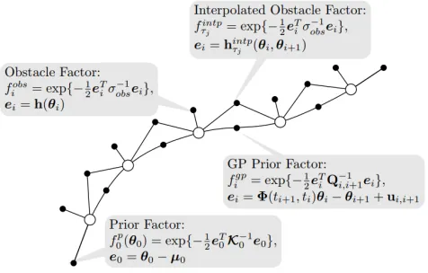
Fig. 1. This figure illustrates how a trajectory can be represented as a factor graph, which includes support states (white circles) and four kinds of factors (black dots). While start and goal factors are respectively placed at the head and tail of the trajectory, GP prior factors serve as a connection between two consecutive support states, and finally the environmental information is conveyed via obstacle and interpolated obstacle factors.
p(θ)∝exp
−1
2kθ−µk
2
K
As mentioned in [8], this prior distribution can be used for encoding the system dynamics via a structured GP in robot state estimation problems. Another important distribution need to be considered is the likelihood function l(θ;e) =
p(e|θ)∝exp
−1
2kh(θ, e)kΣ , whereeis a binary event or
observation value, andh(θ, e)can be any vector-value cost function with covariance matrix Σ. Combined together, our final problem for finding the desired trajectoriesθ(t)can be solved via themaximum a posterior (MAP) computing ofθ θ∗=argmaxθp(θ|e) =argmaxθp(θ)l(θ;e) (1) To effectively solve the optimization problem in Equation 1, the authors further exploit the use offactor graphto de-compose the posterior distributions into different components which correspond to different aims of the robot. For example, let turn the original posterior distribution into a factorized form
p(θ|e)∝ M
Y
m=1
fm(Θm), (2)
wherefmare factors on variable subsetsΘm.
In particular, one can treat the objectives of trajectories optimization problem as different factors which is illustrated in Figure 1. First factor would be Prior Factor, fstart(θ
0)
andfgoal(θ
N)which defines the prior distributions on start and goal states respectively
fip(θi) = exp
−1
2kθi−µik
2 Σ
, i= 0or N (3) Then, GP Prior Factor fgp = Q
if gp
i (θi, θi+1) is used
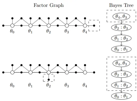
Fig. 2. Examples of Bayes Trees in replanning procedure. Parts of the factor graphs and its correspondingly affected leaves of Bayes Tree are indicated in dashed boxes.
(LTV-SDE), further details can be found on [8]. Finally, to make the robot move safely towards a goal, two types of obstacle cost are also employed, Obstacle Factor fobs
i and
Interpolated Obstacle Factorfτintpi which can be represented as one big obstacle factor
fobs= N
Y
i=0
fiobs(θi)
nip
Y
j=1
fτintpi (θi, θi+1)
= N
Y
i=0
exp
−1 2kh(θi)k
2
σobs
nip
Y
j=1
exp
−1 2kh
intp
τi (θi, θi+1)k 2
σobs
(4)
The final form of the trajectory optimization problem after factorizing can be seen as
θ∗=argmaxθp(θ|e) =argmaxθp(θ)l(θ;e) =argminθ{−log (p(θ)l(θ;e))} =argminθ
−1
2kθ−µk
2
K+ 1 2kh(θ)k
2 Σ
(5)
The apparent construction of the posterior distribution is reduced to a nonlinear least squares problem and then can be solved with any non linear solver like Gaussian Newton or Levenberg-Marquardt. However, using such solver is computational inefficient due to the uncertainty generated in real world scenarios which requires a robot re-solving the optimization problem several time.
To help the re-planning execution more effectively, iSAM2 [9] is applied due to the aforementioned duality between tra-jectories optimization and probabilistic inference throughout the use of factor graph. iSAM2 is an efficient incremental inference framework which was first proposed to solve the SLAM problem. Intuitively, throughout the use of a new data structure Bayes tree, instead of updating all factors on the
factor graph, only neighboured factor will be updated in the re-planning execution which results in a much faster planning in comparison to the naive approach. Figure 2 shows that the graph updating of the top figure only affects θ4, θ3 factor
while any factors between θ2 except the last one will be
updated on the remaining figure.
B. Simultaneous Trajectories Estimation and Planning
To be able to autonomously navigate in an unknown environment, it requires solving both the problem of tra-jectory estimation (localization) and planning. These two have been successfully tackled in a separate manner for a decade. However, while trajectory estimation look like a backward-looking problem where an executed trajectory need to be re-estimated due to incomplete sensor data, the work of finding a clear path to the desired goal seems to be matched with the forward-looking problem. InSimultaneous Trajectories Estimation and Planning (STEAP) article, the authors propose a new method which tackle both problems simultaneously instead of the traditional two-step approach. Intuitively, similar to previous section, STEAP is heavily relied upon the successful offactor graph. In fact, they first treat both the trajectory estimation and planning problem into one single problem and then apply the exact solver and re planning algorithm to tackle this problem. Thus, the whole work of STEAP seems to be inclined on the designing of a suitable factor graph.
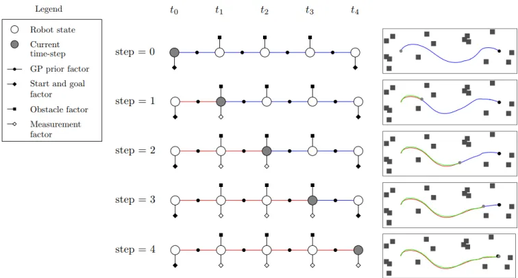
Figure 3 shows an example of STEAP as a simple solution for navigation problem. First, the graph is constructed with five different robot states, equivalent to five different time step which are connected via GP factors that collectively form a prior distribution of a continuous-time trajectory. Then,start and goal factorin addition with a set ofobstacle factor are added to make a mobile robot navigate from current position to the desired goal without collided. Start, goal and obstacle factors together form the likelihood or planed path, correspond to the blue line in Figure 3. Next, in each execution step, the robot incrementally updates the state with current measurement factor, form a new factor graph and eventually resolve the MAP problem by updating the Bayes Tree via iSAM2 algorithm.
III. METHODOLOGIES A. GP Priors
As mentioned earlier, GPMP2 can be seen as a gen-eral framework for tackling different trajectory optimization problems. Two has been solved in the previous sections which areMotion PlanningandMobile Navigation, thus by designing a suitablefactor graph, one can benefit from the efficient in planning and execution of the aforementioned framework without further modification. In fact, while both GPMP2 and STEAP aim to solve the same problem - moving a robot towards the desired goal without collided, GPMP2 focus on manipulation task, and STEAP tackle the mobile robotnavigation problem. The main difference between these two is due to the difference from dynamical systems, thus,
Fig. 3. This figure illustrates how a navigation procedure is represented throughout STEAP, a gray and black circle are represented for the robot and the desired goal, respectively. At each step, three different trajectories are drawn in both factor graphs and the simulated environment, includes ground-truth (green), estimated (red), and replanned (blue) trajectories.
of using a trivial Gaussian kernel such as RBF, both STEAP and GPMP2 are relied upon the linear time varying (LTV) stochastic differential equations (SDEs) GP priors which is proposed in [2]. These priors are highly structured and factorized according to
fgp=Y i
figp(θi, θi+1) (6)
where any GP prior factor connects to only its two neigh-boring states, forming a (Gauss-Markov) chain. In specific, a constant-velocity model p¨(t) = w(t) with N-dimensional position variablep(t), is employed to define a LTV-SDE
˙
θ(t) =A(t)θ(t) +u(t) +F(t)w(t) (7) where θ(t) =
p(t) p˙(t)T
, u(t) is the control input,
A(t) andF(t)are time-varying system matrices, and even-tually the white process noisew(t)which is represented by
w(t)∼GP(0, QCδ(t−t0)) (8) where Qc is the hyperparameter power-spectral density matrix, δ(t−t0) is the Dirac delta function. We refer the reader to [2] for further details. Next, to form an exact
constant-velocity model, u(t), A(t) and F(t) need to be defined as
A(t) =
0 1 0 0
, u(t) = 0, F(t) =
0 1
(9) Once formed the LTV-SDE final formulation, according to [2], one can define the GP factor between any two states at
ti andti+1 as follow
figp(θi, θi+1) = exp
−1
2kΦ(ti+1, ti)θi−θi+1k
2
Qi,i+1
(10)
where the covariance matrix Qi,i+1 =
1 3∆t
3
iQc 12∆t2iQc
1 2∆t
2
iQc ∆tiQc
, and transition functionΦ(ti+1, ti)is defined below ifp(t)is a purely value-vector (configuration vector) as the case defined in GPMP2 framework
Φ(t, s) =
1 (t−s)1
0 1
(11) On the other hand, not all robots’ configuration spaces can be well represented in vector spaces. For example, the orientation of mobile robot in planar space cannot be treated as vectors without singularity (Euler angle) or extra degrees (quaternion). Thus, to be able to apply theconstant velocity
model directly, STEAP adopt the linearization on the Lie group to transform the state θ(t) ∈ SE2 to ξ(t) ∈ RN. However, it not easy to employs this method to control a differential drive robot due to the non-holonomic constraint on the kinematic system. Therefore, in this implementation, to embed such constraint, we incline to use a simpler approach where the pose of robot on canonical coordinates
p(t) =
x(t) y(t) φ(t)T
∈R3 is represented as system state, and then employs the use of differential drive kinematic equation to form the velocitiesp˙(t)
˙
p(t) =
˙
x
˙
y
˙
φ
=
cosφ 0 sinφ 0 0 1
v ω
(12)
wherev andwis linear and angular velocities command, respectively.
On the contrary, in the execution process, by treating the system state as a combined vector between position and velocity states θ(t) =
p(t) p˙(t)T
large, which will cause the tradeoff between computational efficiency and feasibility. Thus, instead of using the raw velocities, we apply the controller which provably stable viaLyapunov functionand computational efficiency from the work [11].
v= vmax
1 +βkκkλ, ω=κv (13) wherevmax, λ, β are hyperparameters, and κis defined as follow
κ=−1
r
k2(δ−arctan (−k1θ)) +
1 + k1 1 + (k1θ)2
sinδ
(14) wherek1 andk2 are shape and gain parameters,
respec-tively; and
r(t) θ(t) δ(t)T
is the transformed state on egocentric polar coordinate of two consecutivesupport state
x(t) y(t) φ(t)T
and
x(t0) y(t0) φ(t0)T
.
B. Global potential factor
The current implementation of STEAP1 poses many chal-lenges which may produce an unstable or infeasible so-lution when dealing with the unstructured in real-world environment. First, STEAP currently uses a very simple initialization strategy where the whole initial trajectory is just the difference between the start and goal pose; and due to heavily relied on the iterative optimization engine, a poor initial solution may lead the optimization algorithm to a bad local optimum area. Next, a subsequent problem is caused by the use of Prior factor at goal state in Equation 3. In fact, due to the local update procedure of the iterative based optimization, experimentally, terminating at the exact goal pose becomes difficult or infeasible if the desired goal is located at a narrow place or surrounded by walls. This difficulty is also partly caused by the use of hinge loss in
Obstacle factor in Equation 4 due to the fact that hinge loss is fundamentally a non-smooth function, which exists an indifferentiable point in the function domain.
To deal with these dilemmas, instead of planning and executing the mobile robot directly via STEAP, we treated it as a local planner module by adopting the results from
global plannerto guide the optimization procedure, like the traditional approach. While the final discrete path which is given by global planner (Dijkstra) is used for better initialization, to guide the robot to the near-goal region without collided, we employ thepotential function factor
fipot(θi) = exp
−1 2
Potential(θi)
2 Σ
(15)
Potential functionreturn the cost at any given pose, which follows the rule ”the lower the cost the nearer the goal”. In addition, by imposing a higher cost for occupied regions, it ensures that no intervened obstacle appears on the returned path. Potential function is also a continuous differentiable function, thus obviously eliminate the potential problem
1https://github.com/gtrll/piper
which is caused by hinge loss. However, one of the main drawbacks of this method is the tradeoff between accuracy and stability it causes, by guiding the robot towards a low-cost region instead of the exact goal, it ensures that the optimizer must generate the trajectory that follows theGlobal planner, thus more stable but low accuracy. Fortunately, this tradeoff can be mitigated by adjusting the resolution of the potential function. The higher resolution would strictly penalize the optimizer if the robot is situated in high-cost regions rather than the near-goal one.
C. Pseudo code
In this section, the wholeextended STEAPframework for differential drive robot navigation is described as follow
Algorithm 1 Extended STEAP
Input: planner path: Planner path,potential: Potential func-tion,θ: trajectory,f: factor, T: Bayes tree
Initialization :
1: θinit = initializeTrajectory(planner path)
2: FG = createFactorGraph(fgp,fpot,potential,ff ix)
3: θ = inference(FG,θinit)
4: T = createBayesTree(FG,θ)
Execution:
5: fori= 0 toN−1do 6: u= controlLaw(θ,i,i+ 1)
7: execute(u)
8: fimeas+1 = localize()
9: θ,T = incrementalInference(θ,fimeas+1 ,T)
10: end for 11: return success
As illustrated, the main difference between two version of STEAP is the initial factor graph and the executing velocities. First, at line 2 of Algorithm 1, the obstacle factor fobs is replaced by the potential one fpot which is described in Equation 15. Meanwhile, instead of computing the command outputu=v ωT
throughout interpolation, at line 6, we apply the controlLaw formula from Equation 13 at current time step of two consecutive support state θi andθi+1 and send this to robot via executefunction in the
following line.
IV. EXPERIMENTAL RESULTS A. Experimental setup
In this section, two experiments are conducted. While the first experiment shows the power of the potential factor in planning, the latter focus on illustrating how the aforemen-tioned Lyapunov provably stable controller [11] serves for the purpose of an efficient execution. In addition, Robot Operation System2(ROS) is heavily employed in this imple-mentation. It is chosen due to the flexibility in transferring between simulation and real-world robot. For simplicity, all experiments are run throughout the STAGE3 which in
2https://ros.org
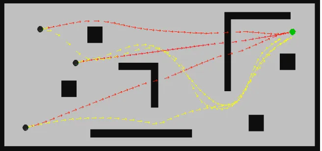
Fig. 4. An experimental result shows the planned trajectories resulted from the original STEAP (red) and our extended version (yellow) in a complicated and unstructured environment. A robot is initially located at three different position (black circle) are searching for a free-collision path towards the goal (green circle).
turn is one of the most popular simulation frameworks for robot navigation task in planar terrain. This implementation is based on the open source framework GTSAM4 where the non-linear solver Levenberg-Marquardt and replanning iSAM2 algorithms are employed. Meanwhile, throughout the implementation of our algorithm, Dijsktra was used as a global planner under ROS navigation stack framework. Be-side those qualitative comparisons, it also worth to mention the computational time of the aforementioned method. Thus, to be specific, all the experiments are run on a desktop with CPU Xeon v1350, 16 Gb RAM, and GPU NVIDIA GTX 1060.
B. Planning
To begin with, the aim of this experiment is to show how the potential factor benefits in making a feasible plan toward a goal in an unstructured environment like the one in Figure 4. As illustrated, a differential drive robot is situated in three different start position, corresponding to the filled black circle in the figure, are all planning toward the green goal location. The resulted trajectories found by STEAP and our extended version are shown under red and yellow set of arrows, respectively. As shown, in all three case, due to the unstructured and complicated of the environment, it obvi-ously shows that without the help of a global planner, STEAP failed to find a path toward the desired goal. Meanwhile, our method not only successfully gives the robot a free-collision path, but also in a reasonable time which is described in Table I.
TABLE I
COMPUTATIONAL TIME OF PLANNERS
STEAP Our
Top 6.9954 0.6498 Middle 9.2135 0.4751 Bottom 7.0078 0.1862
4https://bitbucket.org/gtborg/gtsam/
In Table I, with three different start position - top, middle and bottom, it clearly shows that our method outperformed STEAP in term of time complexity. While in all case, STEAP requires a large number of iteration to reach the final trajectory (but still infeasible), our version successfully found a feasible one in only about half of second.
C. Executing
Next experiment will show how much important the con-trol law [11] is in the execution of differential drive mobile robot. For simplicity, instead of the previously complicated environment, a simpler scenario5 will be considered in this case. That is, a simple trajectory which is a result of our planning strategy requires the robot to reach the desired goal in 20 seconds with 40 support states. To illustrate the power ofestimationandplanning, two evaluation metrics are employed in this experiment. While the former (Equation 16) shows the Euclidean distance between the ground-truth ter-minated pose and the oracle goal (from our planner), the accumulated distance between estimated and ground-truth state (Equation 17) is evaluated in the latter case.
errorplan=kθend−gtendk2 (16)
errorest=
X
i
kθi−gtik2 (17)
Moreover, in order to deal with uncertainty, we ran the robot 5 times and report the average, min and max error in these following table
TABLE II GOAL ERRORS
Raw Our
Average 1.1487 0.2144 Max 1.4633 0.3511 Min 0.8768 0.0943
TABLE III
ACCUMULATED ESTIMATION ERRORS
Raw Our
Average 28.1654 8.6189 Max 30.4067 10.8772 Min 24.3155 4.7663
As illustrated, without the control law, both the estimated and goal-based error are significantly larger than the used one. To be specific, Table II shows that the generated error between oracle and true goal of the one uses control law command, on average, is five times lesser than the raw one. Meanwhile, the estimation accuracy between the estimated and ground-truth path also witness a remarkable improvement. That is, in Table III, it shows that the average estimation error is significantly different (about three times smaller) between two execution strategy. This proves that the accurate execution towards planned ahead way points significantly contribute to the reduction of backward state estimation error.
V. CONCLUSIONS
This work has shown a potential research direction for efficiently controlling and navigating a highly dimensional robot (9 DOF mobile manipulation) in a complex and un-structured environment. To be successfully manipulated, it includes two sequential phase; first, the robot needs to search for a free-collision path towards the goal and then effectively executing it. This can be seen as an analogy to the global and local planner procedure in general navigation framework. Specifically, in this work, while the optimizer is initialized and guided by global planner via potential factor, the iSAM2 [9] re-planning technique plays a role as a local planner where only needed factors are updated instead of resolving the entire optimization problem from scratch. Interestingly, rather than applying the raw velocities resulted from the opti-mizer, we proved that the robot can gratefully and accurately reach a planned ahead waypoint throughout the provably stable controller. However, for simplicity, Dijkstra serves as a global planner throughout this paper, thus, only the efficiency of planar navigation is shown. In future work, we would explore the capability of different sampling-based planners [4] to control the whole body (included attached arm) in a cluttered environment. Generally speaking, one of the main drawbacks of motion planning is about lacking skills from kinesthetic teaching rather than the manually designed cost. Thus, another interesting direction would be discovered the possibility of factor graphs when dealing with different objective functions. One of such is the potential of combining reinforcement learning to account for demonstrated trajectory from human [12].
REFERENCES
[1] F. Dellaert and M. Kaess, “Square root sam: Si-multaneous localization and mapping via square root
information smoothing,”Int. J. Rob. Res., vol. 25, no. 12, 2006.
[2] S. Anderson, T. D. Barfoot, C. H. Tong, and S. Sarkka, “Batch nonlinear continuous-time trajectory estima-tion as exactly sparse gaussian process regression,”
Autonomous Robots, vol. 39, no. 3, pp. 221–238, 2015. [3] L. Kavraki, P. Svestka, J.-C. Latombe, and M. Over-mars, “Probabilistic roadmaps for path planning in high-dimensional configuration spaces,” IEEE Trans-actions on Robotics and Automation, vol. 12, no. 4, pp. 566–580, 1996.
[4] J. Kuffner and S. LaValle, “RRT-connect: An efficient approach to single-query path planning,” in Proceed-ings 2000 ICRA. Millennium Conference. IEEE In-ternational Conference on Robotics and Automation. Symposia Proceedings (Cat. No.00CH37065), IEEE. [5] N. Ratliff, M. Zucker, J. A. Bagnell, and S. Srinivasa,
“CHOMP: Gradient optimization techniques for effi-cient motion planning,” in 2009 IEEE International Conference on Robotics and Automation, IEEE, 2009. [6] M. Zucker, N. Ratliff, A. D. Dragan, M. Pivtoraiko, M. Klingensmith, C. M. Dellin, J. A. Bagnell, and S. S. Srinivasa, “CHOMP: Covariant hamiltonian op-timization for motion planning,” The International Journal of Robotics Research, vol. 32, no. 9-10, pp. 1164–1193, 2013.
[7] M. Kalakrishnan, S. Chitta, E. Theodorou, P. Pastor, and S. Schaal, “STOMP: Stochastic trajectory opti-mization for motion planning,” in2011 IEEE Interna-tional Conference on Robotics and Automation, IEEE, 2011.
[8] M. Mukadam, J. Dong, X. Yan, F. Dellaert, and B. Boots, “Continuous-time gaussian process motion planning via probabilistic inference,” The Interna-tional Journal of Robotics Research, vol. 37, no. 11, pp. 1319–1340, 2018.
[9] M. Kaess, H. Johannsson, R. Roberts, V. Ila, J. J. Leonard, and F. Dellaert, “iSAM2: Incremental smoothing and mapping using the bayes tree,” The International Journal of Robotics Research, vol. 31, no. 2, pp. 216–235, 2011.
[10] M. Mukadam, J. Dong, F. Dellaert, and B. Boots, “STEAP: Simultaneous trajectory estimation and plan-ning,”Autonomous Robots, 2018.