Weakness of F_{3^{6*1429}} and F_{2^{4*3041}} for Discrete Logarithm Cryptography

CRYPTOGRAPHY

GORA ADJ, ALFRED MENEZES, THOMAZ OLIVEIRA, AND FRANCISCO RODR´IGUEZ-HENR´IQUEZ

Abstract. In 2013, Joux and then Barbulescu et al. presented new algorithms for computing discrete logarithms in finite fields of small characteristic. Shortly thereafter, Adj et al. presented a concrete analysis showing that, when combined with some steps from classical algorithms, the new algorithms render the finite field F36_·509 weak for

pairing-based cryptography. Granger and Zumbr¨agel then presented a modification of the new algorithms that extends their effectiveness to a wider range of fields.

In this paper, we study the effectiveness of the new algorithms combined with a carefully crafted descent strategy for the fields F36_·1429 andF₂4_·3041. The intractability

of the discrete logarithm problem in these fields is necessary for the security of pairings derived from supersingular curves with embedding degree 6 and 4 defined, respectively, over F31429 and F₂3041; these curves were believed to enjoy a security level of 192 bits

against attacks by Coppersmith’s algorithm. Our analysis shows that these pairings offer security levels of at most 96 and 129 bits, respectively, leading us to conclude that they are dead for pairing-based cryptography.

1. Introduction

LetFqdenote a finite field of orderq, and letEbe an elliptic curve defined overFq with #E(Fq) =crwhereris prime with gcd(r, q) = 1 andc≪r. Letkbe the embedding degree ofE, i.e., the smallest positive integer satisfyingr |qk−1. The Weil and Tate pairings can be used to reduce the discrete logarithm problem (DLP) in the order-r subgroup ofE(Fq) to the discrete logarithm problem in the order-r subgroup of F∗

qk [10, 18]. Hence, the

security of cryptosystems implemented using elliptic curves with small embedding degrees is dependent on the intractability of the DLP in (the multiplicative group of) Fqk.

Elliptic curves having small embedding degreek have been used to implement pairing-based protocols [4, 6]. In this paper, we are interested in the k= 4 supersingular elliptic curves Y2 +Y = X3 +X and Y2 +Y = X3 +X+ 1 defined over characteristic-two finite fields, and the k = 6 supersingular elliptic curves Y2 _{= X}3_{−X±1 defined over}

characteristic-three finite fields.

The security of these elliptic curves has been severely tarnished due to the recent al-gorithms of Joux [14], G¨olo˘glu et al. [11], and Barbulescu et al. [3]. More precisely, Joux developed an LQ[1₄ +o(1), c] DLP algorithm in FQ, where Q=qn is a power of 2, and q and nare balanced in the sense thatq ≈m wheren= 2m. Here,LQ[α, c] with 0< α <1 and c >0 denotes the expression

exp (c+o(1))(logQ)α(log logQ)1−α

Date: November 14, 2013; updated on November 30 2013.

This work was done while the first, third and fourth authors were visiting the University of Waterloo.

that is subexponential in logQ. Shortly thereafter, Barbulescu et al. presented a new DLP algorithm which, for many choices of field sizes, is asymptotically faster than all previous algorithms. In particular, in the case whereqis a power of 2 or 3 withq ≈nandn≤q+2, the DLP in Fq2n =F_Q can be solved in quasi-polynomial time

(logQ)O(log logQ).

While the new quasi-polynomial time algorithm (QPA) of Barbulescu et al. is asymp-totic in nature (see §2), Adj et al. [1] showed that, when combined with some steps from classical algorithms, they can have a considerable impact on the security of pairing-based protocols in practice. Let E denote the supersingular elliptic curve Y2 = X3−X+ 1 over F3509. Then #E(F₃509) = 7r where r is an 804-bit prime. The finite field F₃6·509 offers approximately 128 bits of security against attacks on the DLP by Coppersmith’s algorithm [8] (see [16]). However, the concrete analysis in Adj et al. demonstrates that the order-r subgroup of the multiplicative group of this field offers at most 82 bits of security against the new attacks of Joux and Barbulescu et al.

The setup in Joux’s algorithm imposes some restrictions on the algorithm parameters which limits the range of fields on which the algorithm is effective. Suppose that one wishes to compute logarithms in Fq2n,1 where q is the power of a small prime and n is prime.

Joux’s algorithm represents Fq2n asF_q2[X]/(I_X), whereI_X is a degree-nirreducible factor of h1Xq−h0 inFq2[X], andh₀, h₁ ∈F_q2[X] have small degree (say, 2); hence, one must have n≤q+ 2. For example, logarithms in F36·509 can be computed by first embedding the field in the quadratic extension F(36₎2·509; one can take q = 36 = 729 and n = 509. However, if one wishes to compute logarithms inF36·1429, then the smallest extension that meets the setup criteria is F(39₎2·1429; this field is too large for the new attacks to be effective.

At ECC 2013, Granger and Zumbr¨agel [12] presented a modification of the new al-gorithms that alleviates the aforementioned restrictions. Their idea is to select IX as a degree-nirreducible factor ofh1(Xq)·X−h0(Xq), whereh0, h1 ∈Fq2[X] have small degree (say, 2); the condition on q and n is then relaxed ton≤2q+ 1. While this modification does not affect the asymptotic run time of the new algorithms, it is very successful in increasing the effectiveness of the new algorithms in practice. For example, the k = 4 elliptic curveE :Y2+Y =X3+X over F21223 has #E(F₂1223) = 5r wherer is a 1221-bit prime. The finite field F24·1223 offers approximately 128 bits of security against attacks on the DLP by Coppersmith’s algorithm. However, by embedding _F24·1223 in F(210)2·1223, Granger and Zumbr¨agel reported that the order-rsubgroup of the multiplicative group of

F24·1223 offers at most 95 bits of security against the new attacks. As a second example, one can embed F36·1429 in F₍₃6₎2·1429 and then the condition n ≤ 2q+ 1 is satisfied with q = 36 _{and n= 1429.}

The purpose of this paper is to show that the new algorithms of Joux and Barbulescu et al., as modified by Granger and Zumbr¨agel, can have a drastic impact on the security of thek= 4 andk= 6 supersingular elliptic curves at higher security levels. More precisely, we consider the k = 6 elliptic curve E1 : Y2 = X3−X −1 over F31429 and the k = 4

1_{In general, one wishes to compute logarithms inF}

pℓn where pis a small prime and nis prime. To

accomplish this, one embeds Fpℓn in F_(pb₎cn where c >1 andℓ|bc. In this paper, we will only consider

elliptic curve E2 : Y2 +Y = X3 +X over F23041. We have #E1(F31429) = cr where r

is a 2223-bit prime and c is a 43-bit cofactor, and #E(F23041) = r where r is a 3041-bit

prime. The finite fieldsF36·1429 andF₂4·3041 offer approximately 192 bits of security against attacks on the DLP by Coppersmith’s algorithm. In contrast, our concrete analysis shows that the order-r subgroups of the multiplicative groups of these fields offer, respectively, at most 96 of security against the new attack with the Granger-Zumbr¨agel polynomial representation, and 129 bits of security against the new attack with Joux’s polynomial representation.

The remainder of the paper is organized as follows. In§2, we elaborate on the “asymp-totic nature” of the Barbulescu et al. algorithm. In §3 we review the DLP algorithms of Joux and Barbulescu et al. as modified by Granger and Zumbr¨agel. Our concrete analyses forF36·1429 andF24·3041 are then presented in §4 and§5.

2. On the asymptotic nature of the QPA algorithm

LetEdenote the supersingular elliptic curveY2_{+Y =X}3_{+X orY}2_{+Y =X}3_{+X+ 1}

over F2n where nis prime, and suppose that #E(F₂n) =cr wherer is prime and c≪r.

The Weil and Tate pairings reduce the discrete logarithm problem in the order-rsubgroup of E(F2n) to the discrete logarithm problem in the order-r subgroup of the multiplicative

group of F24n. Coppersmith’s subexponential-time algorithm [8] can be used to solve the

latter problem.

In constrast, the QPA algorithm of Barbulescu et al. [3] tackles the problem by embed-dingF24n inF_q2n whereq= 2ℓ≈n. The running time of the QPA algorithm is dominated

by the descent stage. In this stage, one begins with a polynomial of degree (at most)n−1 over Fq2 whose logarithm is sought. One then expresses the logarithm of this polynomial in terms of the logarithms of roughlyq2 polynomials of degree at mostn/2. This process is applied recursively to each polynomial encountered in the “descent tree”; the logarithm of each such polynomial of degree d is expressed in terms of the logarithms of roughly q2 polynomials of degree at most d/2. To terminate the recursion, the logarithms of all degree-1 polynomials are obtained using a relatively fast method.

The number of nodes in the descent tree gives a crude lower bound on the running time of the QPA algorithm. Since n≈q, the descent tree has approximately log₂q levels and at least q2 log2q _{nodes. Table 1 compares this lower bound with the running time} C(q) = exp(1.526(log 24q₎1/3_{(log log 2}4q₎2/3_{) of Coppersmith’s algorithm for computing}

discrete logarithms in F24q.

We see from Table 1 that the QPA algorithm is faster than Coppersmith’s algorithm only when n≈q = 215. However, such n are too large to be of interest in cryptography based on pairings overE(F2n). To determine the implications of the QPA algorithm to the

security of pairing-based cryptosystems based onE(F2n), it is imperative that the descent

q q2 log2q C(q) 29 ₂162 ₂93

210 2200 2124 211 ₂242 ₂165

212 2288 2219 213 ₂338 ₂290

214 2392 2382 215 2450 2501

Table 1. Comparison of the running time q2 log2q of the QPA algorithm for computing logarithms in Fq2n with q ≈n, and the running time C(q)

of Coppersmith’s algorithm for computing logarithms inF24n.

3. New DLP algorithm of Joux and Barbulescu et al.

The DLP algorithm we describe is due to Joux [14], with a descent step from the quasi-polynomial time algorithm of Barbulescu et al. [3], and a polynomial representation (selection of h0 and h1) due to Granger and Zumbr¨agel [12]. For lack of a better name,

we will call this algorithm the “new DLP algorithm”. The description of the algorithm closely follows the description in [1]; the most important changes are the incorporation of the polynomial selection of Granger and Zumbr¨agel and the use of lattices in the classical descent stage.

Let Fq2n be a finite field where n ≤ 2q+ 1. The elements of F_q2n are represented as

polynomials of degree at most n−1 over Fq2. Let N =q2n−1. Let g be an element of order N in_F∗

q2n, and leth∈F

∗

q2n. We wish to compute log_gh. The algorithm proceeds by

first finding the logarithms of all degree-one (§3.2) and degree-two (§3.3) elements inFq2n.

Then, in the descent stage, log_gh is expressed as a linear combination of logarithms of degree-one and degree-twoFq2n elements. The descent stage proceeds in several steps, each

expressing the logarithm of a degree-D element as a linear combination of the logarithms of elements of degree ≤ m for some m < D. Four descent methods are used; these are described in §3.4–§3.7. The cost of each step is given in Table 2.

Notation. N_q2(m, n) denotes the number of monic m-smooth degree-n polynomials in

Fq2[X],Aq2(m, n) denotes the average number of distinct monic irreducible factors among all monicm-smooth degree-npolynomials inFq2[X], andS_q2(m, d) denotes the cost of test-ingm-smoothness of a degree-dpolynomial inFq2[X]. Formulas for N_q2(m, n),A_q2(m, n) and S_q2(m, n) are given in [1]. For γ ∈ F_q2, γ denotes the element γq. For P ∈ F_q2[X], P denotes the polynomial obtained by raising each coefficient of P to the power q. The cost of an integer addition modulo N is denoted byAN, and the cost of a multiplication in Fq2 is denoted by M_q2. The projective general linear group of order 2 over F_q is de-noted PGL2(Fq). Pq is a set of distinct representatives of the left cosets of PGL2(Fq) in PGL2(Fq2); note that #P_q=q3+q. A matrix a b_{c d}∈ P_q is identified with the quadruple (a, b, c, d).

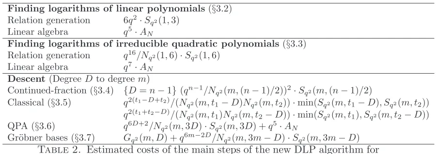
Finding logarithms of linear polynomials(§3.2) Relation generation 6q2_·S

q2(1,3)

Linear algebra q5_·A

N

Finding logarithms of irreducible quadratic polynomials(§3.3) Relation generation q16_/N

q2(1,6)·S_q2(1,6)

Linear algebra q7_·A

N Descent(DegreeD to degreem)

Continued-fraction (§3.4) {D=n−1}(qn₋1_/N

q2(m,(n−1)/2))2·S_q2(m,(n−1)/2)

Classical (§3.5) q2(t1−D+t2)/(N

q2(m, t₁−D)N_q2(m, t₂))·min(S_q2(m, t₁−D), S_q2(m, t₂)) q2(t1+t2₋D)_/(N

q2(m, t₁)N_q2(m, t₂−D))·min(S_q2(m, t₁), S_q2(m, t₂−D))

QPA (§3.6) q6D+2_/N

q2(m,3D)·S_q2(m,3D) +q5·A_N

Gr¨obner bases (§3.7) Gq2(m, D) +q6m−2D/N_q2(m,3m−D)·S_q2(m,3m−D)

Table 2. Estimated costs of the main steps of the new DLP algorithm for computing discrete logarithms inFq2n. A_N andM_q2 denote the costs of an addition moduloN and a multiplication inFq2. See§3.5 for the definitions of t1 and t2. The Gr¨obner basis cost Gq2(m, D) is defined in §3.7.

has an irreducible factor IX of degree n in Fq2[X]; we will henceforth assume that max(degh0,degh1) = 2. Note that

(2) X ≡ h0(X

q₎

h1(Xq) ≡

h0(X)

h1(X)

q

(modIX)

The field Fq2n is represented as F_q2n = F_q2[X]/(I_X) and the elements of F_q2n are

repre-sented as polynomials in Fq2[X] of degree at most n−1. Letg be a generator of F∗_q2n.

3.2. Finding logarithms of linear polynomials. Let B1 = {X+a | a ∈ Fq2}, and note that #B1 =q2. To compute the logarithms of B1-elements, we first generate linear

relations of these logarithms. Let (a, b, c, d) ∈ Pq. SubstitutingY 7→ (aX +b)/(cX+d) into the systematic equation

(3) Yq−Y = Y

α∈Fq

(Y −α)

and then multiplying by (cX+d)q+1 yields

(aX+b)q(cX+d)−(aX+b)(cX+d)q (4)

= (cX+d)· Y α∈Fq

[(a−αc)X+ (b−αd)].

Replacing X by (h0/h1)q in the linear terms aX+b andcX+doccurring in the left side

of (4) and then clearing denominators yields

(aX+b)(ch0+d h1)−(ah0+b h1)(cX+d)

q (5)

≡hq₁·(cX+d)· Y α∈Fq

If the polynomial on the left side of (5) is 1-smooth, then taking logarithms of both sides of (5) yields a linear relation of the logarithms of B1-elements and the logarithm of h1.

The probability that the left side of (5) is 1-smooth is N_q2(1,3)/q6 ≈ 1₆. Thus, after approximately 6q2 trials one expects to obtain (slightly more than)q2 relations. The cost of the relation generation stage is 6q2 _·S

q2(1,3). The logarithms can then be obtained by using Wiedemann’s algorithm for solving sparse systems of linear equations [19]. The expected cost of the linear algebra is q5 _·A

N since each equation has approximately q nonzero terms.

3.3. Finding logarithms of irreducible quadratic polynomials. Let u ∈ Fq2, and let Q(X) = X2 _{+uX +v ∈ F}

q2[X] be an irreducible quadratic. Define B_2,u to be the set of all irreducible quadratics of the form X2 +uX +w in Fq2[X]; one expects that #B2,u≈(q2−1)/2. The logarithms of all elements inB2,u are found simultaneously using one application of QPA descent (see §3.6). More precisely, one first collects relations of the form (13), where the left side of (13) factors as a product of linear polynomials (whose logarithms are known). The expected number of relations one can obtain is Nq2(1,6)

q12 ·(q3+q). Provided that this number is significantly greater than #B2,u, the matrixH(Q) is expected to have full (column) rank. One can then solve the resulting system of linear equations to obtain the logarithms of all irreducible translates Q+w of Q. This step is repeated for each u∈Fq2. Hence, there areq2 independent linear systems of equations to be solved.

For each u ∈ Fq2, the cost of relation generation is q14/N_q2(1,6)·S_q2(1,6), while the linear algebra cost isq5_·A

N.

3.4. Continued-fraction descent. Recall that we wish to compute log_gh, where h ∈ Fq2n = F_q2[X]/(I_X). We will henceforth assume that degh =n−1. The descent stage begins by multiplyinghby a random power ofg. The extended Euclidean algorithm is used to express the resulting field elementh′_{in the formh}′ _=w

1/w2where degw1,degw2≈n/2

[5]; for simplicity, we shall assume that n is odd and degw1 = degw2 = (n−1)/2. This

process is repeated until both w1 and w2 are m-smooth for some chosen m <(n−1)/2.

This gives log_gh′ _{as a linear combination of logarithms of polynomials of degree at most}

m. The expected cost of this continued-fraction descent step is approximately

(6)

qn−1

N_q2(m,(n−1)/2) 2

·S_q2(m,(n−1)/2).

The expected number of distinct irreducible factors of w1 and w2 is 2Aq2(m,(n−1)/2). In the analysis, we shall assume that each of these irreducible factors has degree exactly m. The logarithm of each of these degree-m polynomials is then expressed as a linear combination of logarithms of smaller degree polynomials using one of the descent methods described in §3.5, §3.6 and §3.7.

3.5. Classical descent. Letp be the characteristic of Fq, and let q =pℓ. Let s∈[0, ℓ], and let R ∈ Fq2[X, Y]. For the sake of simplicity, we will assume in this section that h1= 1. Then

h

R(X, hp

ℓ−s

0 )

ips

=R′

(Xps, hp

ℓ

0 ) =R

′

(Xps, h0(Xp ℓ

))≡R′

where R′ _{is obtained fromR by raising all its coefficients to the power p}s_{. Hence}

(7) hR(X, hp

ℓ−s

0 )

ips

≡R′

(Xps, X) (modIX).

Let Q∈Fq2[X] with degQ=D, and let m < D. In the Joux-Lercier descent method [15], as modified by G¨olo˘glu et al. [11], one selectss∈[0, ℓ] and searches for a polynomial R ∈ Fq2[X, Y] such that (i) Q | R₁ where R₁ = R(X, hp

ℓ−s

0 ); (ii) degR1/Q and degR2

are appropriately balanced where R2 = R′(Xp s

, X); and (iii) both R1/Q and R2 are

m-smooth. Taking logarithms of both sides of (7) then gives an expression for log_gQin terms of the logarithms of polynomials of degree at most m.

A family of polynomials R satisfying (i) and (ii) can be constructed by finding a basis

{(u1, u2),(v1, v2)} of the lattice

LQ={(w1, w2)∈Fq2[X]×F_q2[X] : Q|(w₁(X)−w₂(X)h₀(X)p

ℓ−s )}

where degu1, degu2, degv1, degv2≈D/2. The points (w1, w2) in LQ can be sampled to obtain polynomials R(X, Y) =w1(X)−w2(X)Y satisfying (i) and (ii) by writing

(w1, w2) =a(u1, u2) +b(v1, v2) = (au1+bv1, au2+bv2)

with a ∈ Fq2[X] monic of degree δ and b ∈ F_q2[X] of degree δ −1. The number of lattice points to consider is therefore (q2₎2δ_{. We have degw}

1,degw2 ≈ D/2 + δ, so

degR1 =t1 ≈(D/2 +δ) + 2pℓ−s and degR2 =t2 ≈(D/2 +δ)ps+ 1. In order to ensure

that there are sufficiently many such lattice points to generate a polynomial R for which both R1/Qand R2 arem-smooth, the parameterssand δ must be selected so that

(8) q4δ≫ q

2(t1−D)

N_q2(m, t₁−D) ·

q2t2 N_q2(m, t₂).

Ignoring the time to compute a balanced basis of LQ, the expected cost of finding a polynomial R satisfying (i)–(iii) is

(9) q

2(t1−D)

N_q2(m, t₁−D)

· q

2t2

N_q2(m, t₂)

·min(S_q2(m, t₁−D), S_q2(m, t₂)).

The expected number of distinct irreducible factors of R1/Q and R2 isAq2(m, t₁−D) + A_q2(m, t₂). In the analysis, we shall assume that each of these irreducible factors has degree exactly m.

An alternative to the above method is to select s∈[0, ℓ] and search for R∈Fq2[X, Y] such that (i) Q|R2; (ii) degR1 and degR2/Qare appropriately balanced; and (iii) both

R1 and R2/Q are m-smooth. A family of polynomials R satisfying (i) and (ii) can be

constructed by finding a basis {(u1, u2),(v1, v2)} of the lattice

LQ={(w1, w2)∈Fq2[X]×F_q2[X] : Q|(w₁(X)−w₂(X)Xp

s

)}

where degu1, degu2, degv1, degv2≈D/2. The points (w1, w2) in LQ can be sampled as before to obtain polynomialsR(X, Y) =w′′

1(Y)−w′′2(Y)X satisfying (i) and (ii) wherew′′

is obtained fromwby raising all its coefficients to the powerp−s_{. We have degw}

1,degw2 ≈

D/2 +δ, so degR1=t1≈2(D/2 +δ)pℓ−s+ 1 and degR2=t2 ≈(D/2 +δ) +ps. In order

for which both R1 and R2/Qare m-smooth, the parameters s and δ must be selected so

that

(10) q4δ≫ q

2t1

N_q2(m, t₁)

· q

2(t2−D)

N_q2(m, t₂−D) .

Ignoring the time to compute a balanced basis of LQ, the expected cost of finding a polynomial R satisfying (i)–(iii) is

(11) q

2t1

N_q2(m, t₁)

· q

2(t2−D)

N_q2(m, t₂−D)

·min(S_q2(m, t₁), S_q2(m, t₂−D)).

The expected number of distinct irreducible factors of R1 and R2/Q is Aq2(m, t₁) + A_q2(m, t₂−D).

3.6. QPA descent. Let Q ∈ _Fq2[X] with degQ =D, and let m ∈ [⌈D/2⌉, D−1]. Let (a, b, c, d) ∈ Pq. SubstitutingY 7→(aQ+b)/(cQ+d) into the systematic equation (3) and multiplying by (cQ+d)q+1 yields

(12) (aQ+b)q(cQ+d)−(aQ+b)(cQ+d)q= (cQ+d) Y

α∈Fq

[(a−αc)Q+ (b−αd)].

Noticing that

cQ+d≡cQ h0 h1

q! +d≡

cQ

h0

h1

+d

q

≡h−₁DqcQe+d hD₁ q (modIX)

where Qe=hD₁ ·Q(h0/h1), we obtain

(aQ+b)(cQe+d hD₁)−(aQe+b hD₁)(cQ+d) q (13)

≡hDq₁ ·(cQ+d)· Y

α∈Fq

[(a−αc)Q+ (b−αd)] (mod IX).

Note that the polynomial within the main parentheses on the left side of (13) has degree

≤3D. If this polynomial ism-smooth, then (13) yields a linear relation of the logarithms of some degree-m polynomials and logarithms of translates ofQ. After collecting slightly more than q2 such relations, one searches for a linear combination of these relations that eliminates all translates of Qexcept for Qitself. To achieve this, consider row vectors in (ZN)q

2

with coordinates indexed by elementsλ∈Fq2. For each relation, we define a vector v whose entry vλ is 1 if Q−λappears in the right side of (13), and 0 otherwise. If the resulting matrixH(Q) of row vectors has full column rank, then one obtains an expression for log_gQin terms of the logarithms of polynomials of degree≤m. The number of distinct polynomials of degree ≤ m in this expression is expected to be A_q2(m,3D)·q2; in the analysis we shall assume that each of these polynomials has degree exactly m.

Since the probability that a degree-3D polynomial ism-smooth isN_q2(m,3D)/(q2)3D, one must have

(14) Nq2(m,3D)

q6D ·(q

in order to ensure that H(Q) has≫q2 rows, wherebyH(Q) can be expected to have full rank.

The expected cost of the relation generation portion of QPA descent isq6D+2·S_q2(m,3D)/ N_q2(m,3D), while the cost of the linear algebra isq5·A_N.

3.7. Gr¨obner bases descent. LetQ∈Fq2[X] with degQ=D, and letm=⌈(D+1)/2⌉. In Joux’s new descent method [14, §5.3], one finds degree-m polynomials k1, k2 ∈Fq2[X] such that Q|G, where

G= (k1ek2−ek1k2) modIX

and whereek1 =hm1 k1(h0/h1) and ek2 =hm1 k2(h0/h1). We then have

hmq₁ ·k2·

Y

α∈Fq

(k1−αk2)≡G(X)q (mod IX)

as can be seen by making the substitution Y 7→ k1/k2 into the systematic equation (3)

and clearing denominators. Note that deg(ek1) = deg(ek2) = 2m. Hence, if 3m < n then

G=k1ek2−ek1k2 and soG(X) =Q(X)R(X) for someR∈Fq2[X] with degR = 3m−D. If R is m-smooth, we obtain a linear relationship between log_gQ and logs of degree-m polynomials by taking logarithms of both sides of the following:

(15) hmq₁ ·k2·

Y

α∈Fq

(k1−αk2)≡(Q(X)R(X))q (modIX).

To determine (k1, k2, R) that satisfy

(16) k1ek2−ek1k2=Q(X)R(X),

one can transform (16) into a system of multivariate bilinear equations over Fq. Specif-ically, each coefficient of k1, k2 and R is written using two variables over Fq, the two variables representing the real and imaginary parts of that coefficient (which is in Fq2). The coefficients of ek1 andek2 can then be written in terms of the coefficients ofk1 andk2.

Hence, equating coefficients ofXi of both sides of (16) yields 3m+ 1 quadratic equations. The real and imaginary parts of each of these equations are equated, yielding 6m+ 2 bilinear equations in 10m−2D+ 6 variables over Fq. This system of equations can be solved by finding a Gr¨obner basis for the ideal it generates. Finally, solutions (k1, k2, R)

are tested until one is found for whichRism-smooth. This yields an expression for log_gQ in terms of the logarithms of approximately q+ 1 +A_q2(m,3m−D) polynomials of degree (at most) m; in the analysis we shall assume that each of the polynomials has degree exactly m.

Now, the number of candidate pairs (k1, k2) is ((q2)m+1)2 =q4(m+1). Denote byR(m, D)

the expected number of distinct R obtainable. Then the condition

(17) R(m, D)≫ q

2(3m−D)

N_q2(m,3m−D) ,

can ensure that there exists a solution (k1, k2, R) for whichR is m-smooth. The number

It is difficult to determine the exact cost G_q2(m, D) of the Gr¨obner basis finding step. After the Gr¨obner basis is found, the cost to find anm-smoothRis (q2₎3m−D_/N

q2(m,3m− D)·S_q2(m,3m−D).

4. Computing discrete logarithms in _F36·1429

We present a concrete analysis of the DLP algorithm described in §3 for computing discrete logarithms in _F36·1429. In fact, this field is embedded in the quadratic extension field F312·1429, and it is the latter field where the DLP algorithm of §3 is executed. Thus, we have q = 36 _{= 729 andn= 1429.}

As mentioned in §1, our main motivation for finding discrete logarithms inF36·1429 is to attack the elliptic curve discrete logarithm problem in E1(F31429), whereE₁ is the super-singular elliptic curve Y2 _=X3_{−X−1 with #E}

1(F31429) =cr; here c= 7622150170693

is a 43-bit cofactor and r = (31429 −3715+ 1)/c is a 2223-bit prime. The elliptic curve discrete logarithm problem in the order-rsubgroup ofE1(F31429) can be efficiently reduced to the discrete logarithm problem in the order-r subgroup of F∗

312·1429. In the latter prob-lem, we are given two elements α, β of order r in F∗

312·1429 and we wish to find logαβ. It can be readily seen that log_αβ = (log_gβ)/(log_gα) modr, where g is a generator of

F∗

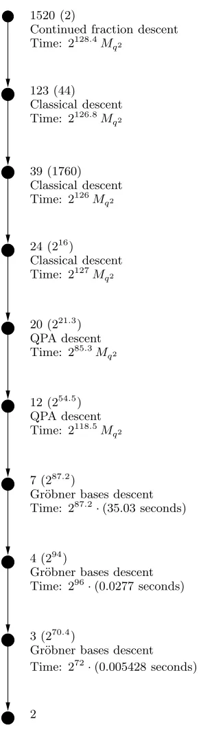
312·1429. Thus, we will henceforth assume that h has order r and that we only need to find log_ghmodr. An immediate consequence of this restriction is that all the linear alge-bra in the new algorithm can be performed modulo the 2223-bit r instead of modulo the 27179-bit N.

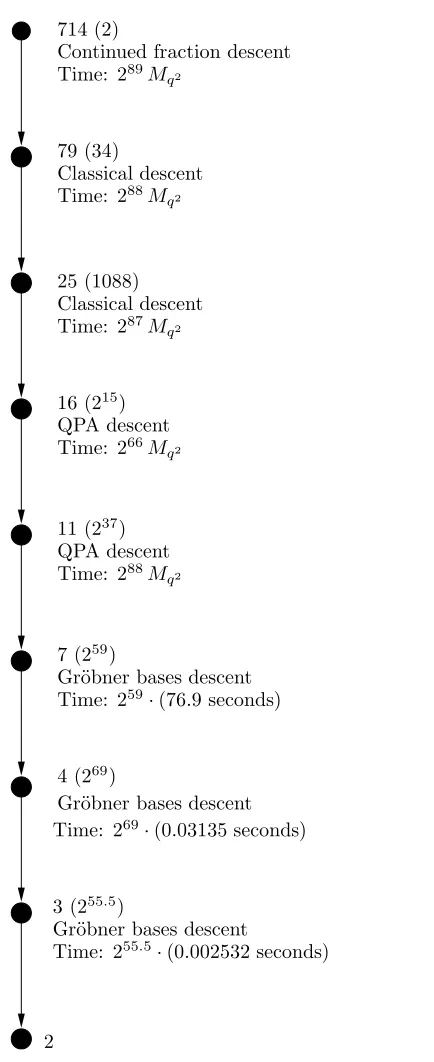
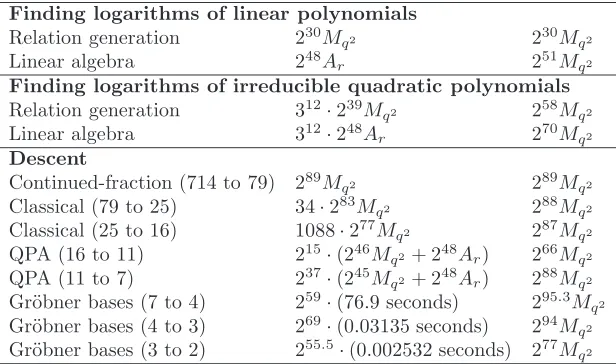
The parameters for each step of the algorithm were carefully chosen in order to balance the running time of the steps. We also took into account the degree to which each step could be parallelized on conventional computers. A summary of the parameter choices for the descent is given in Figure 1. The cost of each step is given in Table 3.

4.1. Setup. We chose the representations F36 = F₃[U]/(U6+ 2U4 +U2+ 2U + 2) and

F312 = F₃6[V]/(V2+U365). We selected h₀ = (U265V +U236)X2+ (U160V +U24)X+ (U628_{V +U}293_{) ∈ F}

312[X] and h₁ = 1, and I_X ∈ F₃12[X] to be the degree-1429 monic irreducible factor of h1(X3

6

)·X−h0(X3

6

). The other irreducible factors have degrees 5, 5 and 19.

4.2. Finding logarithms of linear polynomials. The factor baseB1has size 312≈219.

The cost of relation generation is approximately 230_M

q2, whereas the cost of the linear algebra is approximately 248_A

r.

4.3. Finding logarithms of irreducible quadratic polynomials. For each u∈F312,

the expected cost of computing logarithms of all quadratics in B2,u is 239Mq2 for the computation of H(Q), and 248_A

r for the linear algebra.

Continued fraction descent

Time: 289_M

q2

714 (2)

Classical descent

25 (1088) Classical descent

Time: 287_M

q2

Time: 288_M

q2

QPA descent

Gr¨obner bases descent

Time: 259_{·(76.9 seconds)}

QPA descent 79 (34)

2

3 (255.5₎

Gr¨obner bases descent

Time: 255.5_{·(0.002532 seconds)}

4 (269₎

Gr¨obner bases descent

Time: 269_{·(0.03135 seconds)}

7 (259₎

16 (215₎

11 (237₎

Time: 266_M

q2

Time: 288_M

q2

Finding logarithms of linear polynomials

Relation generation 230_M

q2 230M_q2

Linear algebra 248_A

r 251Mq2

Finding logarithms of irreducible quadratic polynomials

Relation generation 312_·239_M

q2 258M_q2

Linear algebra 312_·248_A

r 270Mq2

Descent

Continued-fraction (714 to 79) 289_M

q2 289M_q2

Classical (79 to 25) 34·283_M

q2 288M_q2

Classical (25 to 16) 1088·277_M

q2 287M_q2

QPA (16 to 11) 215_·(246_M

q2+ 248A_r) 266M_q2

QPA (11 to 7) 237_·(245_M

q2+ 248A_r) 288M_q2

Gr¨obner bases (7 to 4) 259_{·(76.9 seconds) 2}95.3_M

q2

Gr¨obner bases (4 to 3) 269_{·(0.03135 seconds) 2}94_M

q2

Gr¨obner bases (3 to 2) 255.5_{·(0.002532 seconds) 2}77_M

q2

Table 3. Estimated costs of the main steps of the new DLP algorithm for computing discrete logarithms inF312·1429 (q= 3

6_{). A}

r and Mq2 denote the costs of an addition modulo the 2223-bit primer and a multiplication in F312. We use the cost ratio A_r/M_q2 = 23, and also assume that 230 multiplications in F312 can be performed in 1 second (cf. §4.8).

4.5. Classical descent. Two classical descent stages are employed. In the first stage, which uses the alternative method described in §3.5, we have D= 79 and selectm= 25, s = 5, δ = 2, which yield t1 = 247 and t2 = 284. The expected cost of the descent

for each of the 34 degree-79 polynomials is approximately 258.7 ·S_q2(25,205). The ex-pected total number of distinct irreducible polynomials of degree (at most) 25 obtained is approximately 1088.

In the second classical descent stage, which uses the first method described in §3.5, we have D = 25 and select m= 16, s = 2, δ = 2, which yield t1 = 176 and t2 = 127. The

expected cost of the descent for each of the 1088 degree-25 polynomials is approximately 254.4·Sq2(16,127). The expected total number of distinct irreducible polynomials of degree (at most) 16 obtained is approximately 215.

4.6. QPA descent. Two QPA descent stages are employed. In the first stage, we have D = 16 and select m = 11. For each Q, the expected cost of relation generation is 230.9·S_q2(11,48) and the cost of the linear algebra is 248A_r. Also for eachQ, the expected number of distinct polynomials of degree at most 11 obtained is expected to beA_q2(11,48)· q2 ≈222. Thus, the total number of distinct polynomials of degree at most 11 obtained after the first QPA descent stage is approximately 237_.

4.7. Gr¨obner bases descent. Three Gr¨obner bases descent stages are employed. The first stage hasD= 7 and m= 4, and is expected to yield approximately 269 _polynomials

of degree (at most) 4. The second stage has D = 4 and m = 3, and is expected to yield approximately 279 _{polynomials of degree (at most) 3. The third stage has D = 3 and}

m= 2 and is applied to all the 255.5 monic irreducible cubics.

For all three stages, we use the experimental results from §4.7 of [1]. The experiments were run using Magma v2.19-7 [17] on a 2.9 GHz Intel core i7-3520M.

4.8. Overall running time. The second column of Table 3 gives the running time esti-mates for the main steps of the new DLP algorithm in three units of time: Ar,Mq2, and seconds. In order to assess the overall time, we make some assumptions about the ratios of these units of time.

First, we shall assume that Ar/Mq2 = 23. To justify this, we observe that a 2223-bit integer can be stored in 35 64-bit words. The X86-64 instruction set has an ADD opera-tion that adds two 64-bit unsigned integers in one clock cycle. Hence, integer addiopera-tion can be completed in 35 clock cycles. Modular reductions comprises one conditional statement plus one subtraction (required in roughly half of all modular additions). One can use a lazy reduction technique that amortizes the cost of a modular reduction among many integer additions. All in all, the cost of Ar can be estimated to be 35 clock cycles. Unlike for 64-bit integer multiplication, there is no native support for F312 multiplication on an Intel Core i7 machine. However, we expect that a specially designed multiplier could be built to achieve a multiplication cost of 4 clock cycles. This gives us an Ar/Mq2 ratio of approximately 23.

Next, since a multiplication in M_q2 can be done in 4 clock cycles, we will transform one second on a 2.9 GHz machine (on which the Gr¨obner bases descent experiments were performed) into 230Mq2.

Using these estimates, we see from the third column of Table 3 that the overall running time of the new algorithm is approximately 295.8_M

q2. We note that the relation generation, continued-fraction descent, classical descent, and Gr¨obner bases descent steps, and also the relation generation portion of QPA descent, are effectively parallelizable in the sense that one can essentially achieve a factor-C speedup ifCprocessors are available. Moreover, the linear system of equations for finding logarithms of linear polynomials, the 312_≈219_linear

systems of equations for finding logarithms of irreducible quadratic polynomials, and the 215+237linear systems of equations in QPA descent are also effectively parallelizable since each linear system can be solved in less than one day using a small number of GPUs and CPUs (cf. [13] and [2]).

4.9. Comparisons. The upper bound of 295.8M_q2 on the running time of the new algo-rithm for computing logaalgo-rithms inF26·1429 convincingly demonstrates that this field offers drastically less security than the 2192 resistance to attacks by Coppersmith’s algorithm [8, 16]. The decrease in security is even more pronounced when one considers that Copper-smith’s algorithm is non-parallelizable since a dominant step is the solution of an enormous system of linear equations, whereas the new algorithm is effectively parallelizable.

Also striking is the relatively small difference between the 295.8_M

5. Computing discrete logarithms in _F24·3041

We present a concrete analysis of the DLP algorithm described in§3 of [1] for computing discrete logarithms in F24·3041. Note that the algorithm employed in this section uses the original polynomial representationh1Xq−h0of Joux [14]. As with the algorithm described

in§3 of this paper, we employ lattices in the classical descent stages, and use Wiedemann’s algorithm for performing linear algebra.

The fieldF24·3041 is embedded in the sextic extensionF224·3041, and it is in the latter field where the DLP algorithm is executed. Thus, we have q = 212= 2048 andn= 3041.

As mentioned in §1, our main motivation for finding discrete logarithms in F24·3041 is to attack the elliptic curve discrete logarithm problem in E2(F23041), where E₂ is the supersingular elliptic curveY2+Y =X3+Xwith #E2(F23041) =randr= 23041−21521+1 is a 3041-bit prime. The elliptic curve discrete logarithm problem in the order-r subgroup of E2(F23041) can be efficiently reduced to the discrete logarithm problem in the order-r subgroup of F∗

24·3041. We wish to compute logghmodr, where g is a generator of F

∗

24·3041 andh∈F∗

24·3041 has orderr. Hence, all the linear algebra in the new algorithm is performed modulo the 3041-bit r.

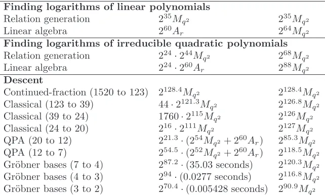
A summary of the parameter choices for the descent is given in Figure 2. The cost of each step is given in Table 4.

Finding logarithms of linear polynomials

Relation generation 235_M

q2 235M_q2

Linear algebra 260_A

r 264Mq2

Finding logarithms of irreducible quadratic polynomials

Relation generation 224_·244_M

q2 268M_q2

Linear algebra 224_·260_A

r 288Mq2

Descent

Continued-fraction (1520 to 123) 2128.4_M

q2 2128.4M_q2

Classical (123 to 39) 44·2121.3_M

q2 2126.8M_q2

Classical (39 to 24) 1760·2115_M

q2 2126M_q2

Classical (24 to 20) 216_·2111_M

q2 2127M_q2

QPA (20 to 12) 221.3_·(254_M

q2+ 260A_r) 285.3M_q2

QPA (12 to 7) 254.5_·(252_M

q2+ 260A_r) 2118.5M_q2

Gr¨obner bases (7 to 4) 287.2_{·(35.03 seconds) 2}120.3_M

q2

Gr¨obner bases (4 to 3) 294_{·(0.0277 seconds) 2}116.8_M

q2

Gr¨obner bases (3 to 2) 270.4_{·(0.005428 seconds) 2}90.9_M

q2

Table 4. Estimated costs of the main steps of the new DLP algorithm for computing discrete logarithms in F224·3041 (q = 212). Ar and M_q2 denote the costs of an addition modulo the 3041-bit primer and a multiplication in F224. We use the cost ratio A_r/M_q2 = 24, and also assume that 228 multiplications in F224 can be performed in 1 second (cf. §5.8).

5.1. Setup. We chose the representationsF212 =F₂[U]/(U12+U7+U6+U5+U3+U+ 1) and F224 = F₂12[V]/(V2 +U152V +U3307). We selected h₀ = (U1515V +U3374)X2 + (U3690_{V +U}2704_{)X + (U}2440_{V +U}142_{) ∈ F}

Continued fraction descent Time: 2128.4_M

q2

1520 (2)

Classical descent

39 (1760) Classical descent Time: 2126_M

q2

Time: 2126.8_M

q2

Classical descent

QPA descent 123 (44)

24 (216₎

Time: 2127_M

q2

Time: 285.3_M

q2

7 (287.2₎

Gr¨obner bases descent Time: 287.2_{·(35.03 seconds)}

2 3 (270.4₎

Gr¨obner bases descent Time: 272·(0.005428 seconds) 4 (294₎

Gr¨obner bases descent Time: 296·(0.0277 seconds) 20 (221.3₎

12 (254.5₎

QPA descent Time: 2118.5_M

q2

IX ∈F224[X] to be the degree-3041 monic irreducible factor of h1·X2

12

−h0. The other

irreducible factors have degrees 5, 7, 69, 110, 293 and 572.

5.2. Finding logarithms of linear polynomials. The factor baseB1 has size 224. The

cost of relation generation is approximately 235_M

q2, whereas the cost of the linear algebra is approximately 260Ar.

5.3. Finding logarithms of irreducible quadratic polynomials. For each u∈F224,

the expected cost of computing logarithms of all quadratics in B2,u is 244Mq2 for the computation of H(Q), and 260_A

r for the linear algebra.

5.4. Continued-fraction descent. For the continued-fraction descent, we selectedm= 123. The expected cost of this descent is 2128.4Mq2. The expected number of distinct irreducible factors of degree (at most) 123 obtained is 2A₂24(123,1520)≈44.

5.5. Classical descent. Let p= 2 and ℓ= 12. Let s∈[0, ℓ], and letR∈Fq2[X, Y] with deg_Y R=e. Then

(18) he₁·hR(X, Xpℓ−s )ip

s

=he₁·R′

(Xps, Xpℓ)≡he₁·R′

(Xps, h0/h1) (mod IX),

where R′

is obtained fromR by raising all its coefficients to the power ps.

LetQ∈Fq2[X] with degQ=D, and letm < D. One selectss∈[0, ℓ] and searches for a polynomialR∈Fq2[X, Y] such that (i)Q|R₁ whereR₁ =R(X, Xp

ℓ−s

); (ii) degR1/Qand

degR2 are appropriately balanced where R2 =he1·R′(Xp s

, h0/h1); and (iii) both R1/Q

and R2 arem-smooth. Taking logarithms of both sides of (18) then gives an expression

for log_gQin terms of the logarithms of polynomials of degree at most m.

A family of polynomials R satisfying (i) and (ii) can be constructed by finding a basis

{(u1, u2),(v1, v2)} of the lattice

LQ ={(w1, w2)∈Fq2[X]×F_q2[X] : Q|(w₁(X)−w₂(X)Xp

ℓ−s )}

where degu1, degu2, degv1, degv2≈D/2. The points (w1, w2) in LQ can be sampled to obtain polynomials R(X, Y) =w1(X)−w2(X)Y satisfying (i) and (ii) by writing

(w1, w2) =a(u1, u2) +b(v1, v2) = (au1+bv1, au2+bv2)

witha∈Fq2[X] monic of degreeδandb∈F_q2[X] of degreeδ−1. We have degw₁,degw₂ ≈ D/2 +δ, so degR1=t1 ≈(D/2 +δ) +pℓ−s and degR2 =t2 ≈(D/2 +δ)ps+ 2. In order

to ensure that the number of lattice points considered is enough to generate a polynomial R such that both R1/Qand R2 are m-smooth, the parameters s and δ must be selected

so that

(19) q4δ≫ q

2(t1−D)

Nq2(m, t₁−D)

· q

2t2

Nq2(m, t₂) .

Ignoring the time to compute a balanced basis of LQ, the expected cost of finding a polynomial R satisfying (i)–(iii) is

(20) q

2(t1−D)

N_q2(m, t₁−D)

· q

2t2

N_q2(m, t₂)

The expected number of distinct irreducible factors of R1/Q and R2 isAq2(m, t₁−D) + Aq2(m, t₂). In the analysis, we shall assume that each of these irreducible factors has degree exactly m.

Three classical descent stages are employed. In the first stage, we have D = 123 and select m= 39, s= 3, δ = 2, which yieldt1 = 575 andt2 = 506. The expected cost of the

descent stage for each of the 44 degree-123 polynomials is approximately 293.7_·S

q2(39,452). The expected total number of distinct irreducible polynomials of degree (at most) 39 obtained is approximately 1760.

In the second classical descent stage we have D= 39 and select m= 24, s= 4, δ = 2, which yield t1 = 277 andt2= 338. The expected cost of the descent for each of the 1760

degree-39 polynomials is approximately 290.2·Sq2(24,238). The expected total number of distinct irreducible polynomials of degree (at most) 24 obtained is approximately 216.

In the third classical descent stage we have D = 24 and select m = 20, s= 4, δ = 2, which yield t1 = 270 and t2 = 226. The expected cost of the descent for each of the 216

degree-24 polynomials is approximately 286.9·S_q2(24,226). The expected total number of distinct irreducible polynomials of degree (at most) 20 obtained is approximately 221.3.

5.6. QPA descent. Two QPA descent stages are employed. In the first stage, we have D = 20 and select m = 12. For each Q, the expected cost of relation generation is 234.8·Sq2(12,60) and the cost of the linear algebra is 260A_r. Also for eachQ, the expected number of distinct polynomials of degree at most 12 obtained is expected to beA_q2(12,60)· q2 _≈233.2_{. Thus, the total number of distinct polynomials of degree at most 12 obtained}

after the first QPA descent stage is approximately 254.5.

In the second stage, we have D= 12 and select m= 7. For each Q, the expected cost of relation generation is 235·Sq2(7,36) and the cost of the linear algebra is 260A_r. Also for each Q, the expected number of distinct polynomials of degree at most 7 obtained is expected to be A_q2(7,36)·q2 ≈232.7. Thus, the total number of distinct polynomials of degree at most 7 obtained after the second QPA descent stage is approximately 287.2_.

5.7. Gr¨obner bases descent. Three Gr¨obner bases descent stages are employed. The first stage hasD= 7 andm= 4, and is expected to yield approximately 299.2 polynomials of degree (at most) 4. The second stage has D= 4 and m = 3 and is applied to all the 294 _{monic irreducible quartics over F}

224. The third stage has D = 3 and m = 2 and is

applied to all the 270.4 monic irreducible cubics overF224. Our experiments were run using

Magma v2.19-7 [17] on a 2.9 GHz Intel core i7-3520M.

In the first stage, for each degree-7 polynomial Qwe have to solve a system of 26 qua-dratic polynomial equations in 32 variables over Fq (cf. (16)). After fixing some variables, each degree-5Robtained from the variety of the resulting ideal is tested for 4-smoothness. If no 4-smooth Ris obtained, we randomly fix some other subset of variables and repeat. We ran 10,000 Gr¨obner bases descent experiments with randomly-selected degree-7 poly-nomials Q. On average, we had to find 1.806 Gr¨obner bases for each Q. The average number of R’s tested for 4-smoothness for each Qwas 1.252. The average time spent on each Q was 35.03 seconds.

For the second and third stages, we use the experimental results from§A.7 of [1].

seconds. In order to assess the overall time, we make some assumptions about the ratios of these units of time.

First, we shall assume that Ar/Mq2 = 24. To justify this, we observe that a 3041-bit integer can be stored in 48 64-bit words. As in §4.8, the cost of Ar can be estimated to be 48 clock cycles. Using the carry-less multiplication instruction PCLMULQDQ, a multiplication in F224 can be performed at a price of 3-4 clock cycles. This gives us an Ar/Mq2 ratio of approximately 24.

Next, since a multiplication in M_q2 can be done in 15 clock cycles, we will transform one second on a 2.9 GHz machine (on which the Gr¨obner bases descent experiments were performed) into 228M_q2.

Using these estimates, we see from the third column of Table 4 that the overall running time of the new algorithm is approximately 2129.3M_q2. The new algorithm is effectively parallelizable, since each linear system of equations can be expected to be solvable in less than 12 days using a small number of GPUs and CPUs (cf. [13, 2]).

5.9. Comparisons. The upper bound of 2129.3Mq2 on the running time of the new algo-rithm for computing logaalgo-rithms inF24·3041 convincingly demonstrates that this field offers drastically less security than the 2192 _{resistance to attacks by Coppersmith’s algorithm}

[8, 16]. As with the case of F36·1429, this decrease in security is even more pronounced when one considers that Coppersmith’s algorithm is non-parallelizable whereas the new algorithm is effectively parallelizable.

References

[1] G. Adj, A. Menezes, T. Oliveira and F. Rodr´ıguez-Henr´ıquez, “Weakness ofF3509for discrete logarithm

cryptography”,Pairing-Based Cryptography – Pairing 2013, to appear; available at http://eprint.iacr. org/2013/446.

[2] R. Barbulescu, C. Bouvier, J. Detrey, P. Gaudry, H. Jeljeli, E. Thom´e, M. Videau and P. Zimmermann, “Discrete logarithm inGF(2809_{) with FFS”, available at http://eprint.iacr.org/2013/197.}

[3] R. Barbulescu, P. Gaudry, A. Joux and E. Thom´e, “A quasi-polynomial algorithm for discrete loga-rithm in finite fields of small characteristic: Improvements over FFS in small to medium characteris-tic”, available at http://eprint.iacr.org/2013/400.

[4] P. Barreto, H. Kim, B. Lynn and M. Scott, “Efficient algorithms for pairing-based cryptosystems”, Advances in Cryptology – CRYPTO 2002, LNCS 2442 (2002), 354–368.

[5] I. Blake, R. Fuji-Hara, R. Mullin and S. Vanstone, “Computing logarithms in finite fields of charac-teristic two”,SIAM Journal on Algebraic and Discrete Methods, 5 (1984), 276–285.

[6] D. Boneh, B. Lynn, and H. Shacham, “Short signatures from the Weil pairing”,Journal of Cryptology, 17 (2004), 297–319.

[7] Q. Cheng, D. Wan and J. Zhuang, “Traps to the BGJT-algorithm for discrete logarithms”, available at http://eprint.iacr.org/2013/673.

[8] D. Coppersmith, “Fast evaluation of logarithms in fields of characteristic two”, IEEE Transactions on Information Theory, 30 (1984), 587–594.

[9] D. Coppersmith, “Solving homogeneous linear equations overGF(2) via block Wiedemann algorithm”, Mathematics of Computation, 62 (1994), 333–350.

[10] G. Frey and H. R¨uck, “A remark concerningm-divisibility and the discrete logarithm in the divisor class group of curves”,Mathematics of Computation, 62 (1994), 865–874.

[11] F. G¨olo˘glu, R. Granger, G. McGuire and J. Zumbr¨agel, “On the function field sieve and the impact of higher splitting probabilities: Application to discrete logarithms inF21971”,Advances in Cryptology –

CRYPTO 2013, LNCS 8043 (2013), 109–128.

[13] H. Jeljeli, “Accelerating iterative SpMV for discrete logarithm problem using GPUs”, available at http://arxiv.org/abs/1209.5520.

[14] A. Joux, “A new index calculus algorithm with complexityL(1/4 +o(1)) in very small characteristic”, Selected Areas in Cryptography – SAC 2013, to appear; available at http://eprint.iacr.org/2013/095. [15] A. Joux and R. Lercier, “The function field sieve in the medium prime case”Advances in Cryptology

– EUROCRYPT 2006, LNCS 4004 (2006), 254–270.

[16] A. Lenstra, “Unbelievable security: Matching AES security using public key systems”, Advances in Cryptology – ASIACRYPT 2001, LNCS 2248 (2001), 67–86.

[17] Magma v2.19-7, http://magma.maths.usyd.edu.au/magma/.

[18] A. Menezes, T. Okamoto and S. Vanstone, “Reducing elliptic curve logarithms to logarithms in a finite field”,IEEE Transactions on Information Theory, 39 (1993), 1639–1646.

[19] D. Wiedemann, “Solving sparse linear equations over finite fields”,IEEE Transactions on Information Theory, 32 (1986), 54–62.

Computer Science Department, CINVESTAV-IPN

E-mail address: [email protected]

Department of Combinatorics & Optimization, University of Waterloo

E-mail address: [email protected]

Computer Science Department, CINVESTAV-IPN

E-mail address: [email protected]

Computer Science Department, CINVESTAV-IPN