Surrounding matter theory

Surrounding matter theory

Frederic Lassiaille1,* 1_{FL research, France}

Abstract. S.M.T. (Surrounding Matter Theory), an alternative theory to dark matter, is presented. It is based on a modification of Newton’s law. This modification is done by multiplying a Newtonian potential by a given factor, which is varying with local distribution of matter, at the location where the gravitational force is exerted. With this new equation the model emphasizes that a gravitational force is roughly inversely proportional to mass density at the location where this force is applied. After presentation of the model, its dynamic is quickly applied to cosmology and galaxy structure. Some possible caveats of the model are identified. But the simple mechanism described above suggests the idea of a straightforward solution to the following issues: virial theorem mystery, the bullet cluster (“1E 0657-56” galaxy clusters) issue, the strong relative velocity of its sub -clusters, the value of cosmological critical density, the fine tuning issue, and expansion acceleration. Nucleosynthesis is not explained and would require a different model for radiation era. But a de Sitter Universe is predicted, this means that the spatial curvature, K, is 0, and today’s deceleration parameter, q, is -1. The predicted time since last scattering is 68 h-1_{Gyr. With this value SMT explains heterogeneities of large scale} structure and galaxy formation. Each kind of experimental speed profiles are retrieved by a simulation of a virtual galaxy. In the simulations, ring galaxies are generated by SMT dynamic itself, without the help of any particular external event. Those studies give motivation for scientific comparisons with experimental data.

1 Introduction

This article presents Surrounding Matter Theory (SMT), and is a very quick survey of its

predictions and results. This model is an alternative to dark matter in solving today’s gravitational mysteries. The solving principle is a modification of Newton’s law. SMT is composed of 1 equation and 2 parameters. This simplicity allows a robust survey of the model, and restricts enormously the amount of possible regression on other parts of physics. Stated in one sentence, the whole behavior of those equations is that a gravitational force is inversely proportional to matter density at the location where the force is exerted.

The first motivation is an old one: Mach’s principle [1]. Here an attempt is made to express

fully this principle by getting the ratio of inertial to gravitational mass, or let’s say a “modified

G

”, directly coupled to matter. And to avoid any resulting changes in the local

behaviour of matter, and the local equations of motion, the first idea is to restrict this

G

variation to large distances only. The second idea is a novelty: relating this variation only to matter located at the location where the force is exerted. This will keep valid linearity with attracting matter. The second motivation concerns General Relativity (GR). Indeed, in GR, Bianchi identity and the resulting null covariant divergence





G

_



0

of

G

_ Einstein tensor is linked directly to energy conservation





T

_



0

of

T

_, the stress-energy tensor, via Einstein equation. But one could notice that the first one comes from pure geometry, whereas the second one comes from physics, namely energy conservation physics principle. This leads me to consider the possibility that those 2 equations are not directly binded together, but could rely on one another through a more complex relation. In particular, I allowed for the Einstein tensor not to be proportional to the stress-energy tensor but rather to be a more general function of it. Furthermore, for reasons such as linearity with respect to energy, I was led to the form

G

_





C C T

_{  }  .



is the multiplicative constant of Einstein equation

G







T

.

C

 is a mixed tensor which remains to be

calculated using the GR case and the non relativistic limit. For the latter this modification undergo to the simple modification of a gravitational potential. This led to

 

C

_SMT



_n, where



is the final gravitational potential.



_n is a Newtonian potential.

C

_SMT is a varying factor, being a function of matter density at the location where the force is exerted.

Today’s gravitational mysteries are solved or partially solved using various different

theories, for example in [2-8]. After the SMT description, its dynamic will be illustrated in the context of the appearance of those mysteries.

2 The model

As introduced above, the starting point is the following gravitational potential equation.

n

MG

_x

 

(1)

x

is the distance from an attracting infinitesimal object,

M

the mass of this object and

G

is gravitational constant. The model consists of modifying this equation. Three more variables are added.

The first one is



, mass density calculated in a sphere of ray

r

max around the location

where the force is applied. This sphere will be called the “SMT sphere” in this document.

There is

r

max= h kpc-1 ,

h

being Hubble constant in units of 100 km s Mpc -1 -1. Using

0

H



_{67 km s Mpc}

_

-1 -1_{, there is kpc}

max

r  . It is this

r

max value which will be used in this document.



0 is today’s value of



in the vicinity of the sun. It will be used:

0





_{0 9810}

_.

_

21

_kg/m

3_{. The modified potential equation is the following.}

0 0 u0

u SMT

MG

x

C

 



 





variation to large distances only. The second idea is a novelty: relating this variation only to matter located at the location where the force is exerted. This will keep valid linearity with attracting matter. The second motivation concerns General Relativity (GR). Indeed, in GR, Bianchi identity and the resulting null covariant divergence





G

_



0

of

G

_ Einstein tensor is linked directly to energy conservation





T

_



0

of

T

_, the stress-energy tensor, via Einstein equation. But one could notice that the first one comes from pure geometry, whereas the second one comes from physics, namely energy conservation physics principle. This leads me to consider the possibility that those 2 equations are not directly binded together, but could rely on one another through a more complex relation. In particular, I allowed for the Einstein tensor not to be proportional to the stress-energy tensor but rather to be a more general function of it. Furthermore, for reasons such as linearity with respect to energy, I was led to the form

G

_





C C T

_{  }  .



is the multiplicative constant of Einstein equation

G







T

.

C

 is a mixed tensor which remains to be

calculated using the GR case and the non relativistic limit. For the latter this modification undergo to the simple modification of a gravitational potential. This led to

 

C

_SMT



_n, where



is the final gravitational potential.



_n is a Newtonian potential.

C

_SMT is a varying factor, being a function of matter density at the location where the force is exerted.

Today’s gravitational mysteries are solved or partially solved using various different

theories, for example in [2-8]. After the SMT description, its dynamic will be illustrated in the context of the appearance of those mysteries.

2 The model

As introduced above, the starting point is the following gravitational potential equation.

n

MG

_x

 

(1)

x

is the distance from an attracting infinitesimal object,

M

the mass of this object and

G

is gravitational constant. The model consists of modifying this equation. Three more variables are added.

The first one is



, mass density calculated in a sphere of ray

r

max around the location

where the force is applied. This sphere will be called the “SMT sphere” in this document.

There is

r

max= h kpc-1 ,

h

being Hubble constant in units of 100 km s Mpc -1 -1. Using

0

H



_{67 km s Mpc}

_

-1 -1_{, there is kpc}

max

r  . It is this

r

max value which will be used in this document.



0 is today’s value of



in the vicinity of the sun. It will be used:

0





_{0 9810}

_.

_

21

_kg/m

3_{. The modified potential equation is the following.}

0 0 u0

u SMT

MG

x

C

 



 







(2)

The second variable is



u, the Universe mass density.



u0 is today’s value of



u. The third variable is



, which can be set to 2 values only. There is

 



0



1 610

.



5 inside

the galaxies, and





1

outside any galaxy. Those values are stated to be independent of Universe expansion.

3 Relativistic version

In the equation giving

C

SMT, through a Lorentz transform, each parameter on the numerator evolves exactly the same way as its corresponding counterpart in the denominator. The result is that

C

SMT is a Lorentz invariant.

The first remark before searching for a relativistic version is the role of

M

in equation (1) and (2). Since

C

SMT depends only on matter at the location where the force is exerted, it does not depend directly on

M

. Therefore like equation (1), equation (2) shows acceleration as being linear with respect to attracting matter (

M

). This is a distinctive

characteristic of SMT as a modification of Newton’s law. Only variations with distance (

x

), and

G

(in some sense, because it is in fact

C G

SMT ) are modified, not variation with

M

. One could even guess that this characteristic would hold with the relativistic version of SMT.

Now modifying Einstein equation with a metric related scalar would not give back equation (2) as the non relativistic limit. It would be the same with any scalar-tensor theory [9], which would finally add a scalar tensor to the physical stress-energy tensor. Einstein modified equation would not show its left-handed term as being strictly linear with respect to attracting energy. Any modification acting on Lagrangian level would probably result in the same caveats, except if modifying the scalar curvature itself in GR Lagrangian. SMT Lagrangian will be given below, but only after calculation of the modified Einstein equation. For this calculation the algebraic constraints are the following.

 Bianchi identity,

 stress-energy tensor conservation,

 variation of

C

SMT,

 linearity of curvature with respect to attracting matter.

The latter implies that any added term is forbidden. Therefore a simple solution is to replace

C

SMT by its space-time tensorial expression.

C

SMT is replaced by

C C

  , where

C



 is a mixed multiplying tensor, allowing a different factor than

C

SMT to be applied to the space components of

T

_. Since the result must retrieve equation (2) in the non-relativistic case, there is

C ² C

00



SMT in the co-moving bases. Bianchi identity and energy conservation along with

C

SMT variation imply a separate variation of each

C

 factor in

front of its corresponding component in the stress-energy tensor. Now this factor depends on the component being multiplied, that is, it depends on



and



. These constraints lead

to the generalization of

1

8

₄

2

G

R

Rg

T

c

  



4

0 0

1

8

2

SMT i i

G

R

Rg

S

c

S

C C T

C

C

C

s

  

     

   





















(3)

c

is the speed of light,

R

_ is the Ricci tensor,

g

_ is the metric,

R

is the trace of

R

_.

 



are Kronecker symbols and

i

indice is varying between 1 and 3. Equations (3) shows that

C

_ is a time dilation by the

C

_SMT factor, and a space dilation by the

s

factor,

s

being a positive scalar. For calculating

s

,





G

_



0

implies the following.



 



  







0 0

00 00

2

0

2

0

i ii

SMT SMT i ii

i i

i i SMT i i

i k kk i k i kk

C

C

sT g

g

sT

C

sT g

g

s T T g

g

































(4)

Here it has been supposed

c



1

for simplification. The notation

   



/ x

 has been

used. The calculation is done in co-moving bases such as

g

_ matrices are diagonal, and supposing no shear forces in

T

_. Therefore

T

_ matrices are also diagonal. Here the non SMT case

C

SMT



1

is simply solved by setting

s



1

. In the general case equations (4) allow a calculation of a finite

s

, but only under the supposition of a non null pressure

0

i i

T



. Otherwise it corresponds to the more general hypothesis of a null stress tensor. And this can be argued as being never completely physically relevant. A static Universe is also forbidden for calculating

s

(exactly there must be



0

g

ii



0

). And it can be argued also that a static Universe is never physically relevant.

Nevertheless, for avoiding those slight caveats, another solution is the following. As

mentioned in the motivation, let’s postulate that the null covariant divergence





G

_



0

of Einstein tensor is independent of energy conservation





T

_



0

, in the general case. This can be modeled by a

S

_ isotropic space part, independent of

T

_. In this case

0

S

 





yields the following, using again the co-moving bases and searching for a diagonal

S

 matrix, but now without any supposition on

T

.



 







0 0

00 00

2

0

2

0

ii SMT SMT SMT ii i SMT SMT SMT i

C

C

P

g

g

P

C

P

g

g

















4

0 0

1

8

2

SMT i i

G

R

Rg

S

c

S

C C T

C

C

C

s

            





















(3)

c

is the speed of light,

R

_ is the Ricci tensor,

g

_ is the metric,

R

is the trace of

R

_.

 



are Kronecker symbols and

i

indice is varying between 1 and 3. Equations (3) shows that

C

_ is a time dilation by the

C

_SMT factor, and a space dilation by the

s

factor,

s

being a positive scalar. For calculating

s

,





G

_



0

implies the following.



 



  







0 0 00 00

2

0

2

0

i ii

SMT SMT i ii

i i

i i SMT i i

i k kk i k i kk

C

C

sT g

g

sT

C

sT g

g

s T T g

g

































(4)

Here it has been supposed

c



1

for simplification. The notation

   



/ x

 has been

used. The calculation is done in co-moving bases such as

g

_ matrices are diagonal, and supposing no shear forces in

T

_. Therefore

T

_ matrices are also diagonal. Here the non SMT case

C

SMT



1

is simply solved by setting

s



1

. In the general case equations (4) allow a calculation of a finite

s

, but only under the supposition of a non null pressure

0

i i

T



. Otherwise it corresponds to the more general hypothesis of a null stress tensor. And this can be argued as being never completely physically relevant. A static Universe is also forbidden for calculating

s

(exactly there must be



0

g

ii



0

). And it can be argued also that a static Universe is never physically relevant.

Nevertheless, for avoiding those slight caveats, another solution is the following. As

mentioned in the motivation, let’s postulate that the null covariant divergence





G

_



0

of Einstein tensor is independent of energy conservation





T

_



0

, in the general case. This can be modeled by a

S

_ isotropic space part, independent of

T

_. In this case

0

S

 





yields the following, using again the co-moving bases and searching for a diagonal

S

 matrix, but now without any supposition on

T

.



 







0 0 00 00

2

0

2

0

ii SMT SMT SMT ii i SMT SMT SMT i

C

C

P

g

g

P

C

P

g

g



























(5)

It has been written

P

SMT



S

11



S

22



S

33. This should allow to calculate

P

SMT in any cases. But here the non SMT case

C

SMT



1

implies either an unrealistic simplification of

the physical stress tensor, or its independence from space-time curvature. Therefore validation of GR equation in the particular context of a non null space part of the stress-energy tensor must be searched for, in order to possibly invalidate this last solution, and then choose the other one. This completes the construction of equations (3). Finally, those equations must be validated backward. And the result is that they fulfill each of their initial

constraints. In the specific case of today’s solar system, SMT prediction is exactly GR. More generally, GR is retrieved in the “constant

C

SMT



1

” case. This is of course mandatory. Equation (2) is retrieved in the non-relativistic case. But in the other cases, differences with GR must be analyzed.

4 Possible regressions

In the “constant

C

SMT ” case, GR is not exactly retrieved: if

C

SMT



1

, there is also

s



1

, with

s C



SMT. Therefore, not only

G

appears to be different, but also a dilatation factor appears on the space part of the stress-energy tensor. This implies that some PPN formalism parameters will be different from their GR values. But comparing those new predicted values with reality would require testing gravity today 15



kpc

beyond the solar system, or inside the solar system but more than

50000



years in the past (since there is

15



kpc

 

50 000



LY

). At first glance those experiments seems difficult to realize.

Even the “varying

C

SMT ” case in which matter density is varying consistently, must be thoroughly analyzed. In particular, a possible time variation of

C

SMT in the solar system must be studied. The resulting apparent

G

variation must be calculated from matter density variation in the SMT sphere around the sun, and then compared to experimental data.

The case of binary stars and exoplanets will be addressed further in this document.

An important case is the spherically symmetric Universe. The Schwarzschild metric behaves like the classical one but with a different

G

value. Here emptiness

T

_



0

leads to a radically unrealistic situation: there is a singularity everywhere in the Universe. And

this is, now, compatible with Mach’s principle. The cosmological case will be addressed

below.

5 Lagrangian version

Let’s review GR Lagrangian:

L

_GR







gRdx

4



L

_M .

g

is the metric determinant

and

L

_M the energy Lagrangian such as

1

8

M

L

T

G g

 



 

 

. Now let’s calculate

L

_SMT,

SMT

R



g D D R

  

  , and

L

CSMT such as

L

CSMT

 





g Xdx

4,

X

being a

scalar such as

X

g R



D D



g

g

 

 

 

 











, there is:

4

SMT SMT M CSMT

L







gR dx



L



L

(6)

It looks like GR Lagrangian.

R

has been replaced by

R

_SMT, which can be interpreted as

R

modified by

C

SMT. An added term,

L

CSMT, has appeared. It can be interpreted as the Lagrangian corresponding to

C

SMT. The following suppositions have been done in order to yield equation (6).

 The mean value of

C

SMT has been supposed constant over the Universe, this “mean” value being calculated over a given distance greater than the visible Universe size.



C

_SMT is supposed to vary around this mean value regularly (that is, with a frequency bounded by a minimum value)

6 Gravitational mysteries

6.1 Aim of these overviews

Some gravitational mysteries will be studied in this document. This will be done in a very quick, mostly qualitative, and carefull manner. These studies are not scientific comparisons. They are only very quick applications of SMT to some particular contexts. Their aim is only to reveal some interesting characteristics of SMT dynamic.

6.2 Critical Universe density

In the context of Friedmann-Lemaître-Robertson-Walker (FLRW) metric, there is

 



u.

This is imposed by Universe homogeneity in this case. First of all, let’s calculate the first

Friedmann-Lemaître (FL) equation.

2 2

2

8

3

SMT u

Kc

G

H

C

a



_





(7)

This result is independent of the choice of the model, that is, the choice between equations (4) or equations (5).

H

is Hubble parameter,

a

is the scale factor, and

K

is space curvature. In FLRW metric context, there is





1

therefore equation (2) shows that

SMT u

SMT

R



g D D R

  

  , and

L

CSMT such as

L

CSMT

 





g Xdx

4 ,

X

being a

scalar such as

X

g R



D D



g

g

       











, there is:

4

SMT SMT M CSMT

L







gR dx



L



L

(6)

It looks like GR Lagrangian.

R

has been replaced by

R

_SMT, which can be interpreted as

R

modified by

C

SMT. An added term,

L

CSMT, has appeared. It can be interpreted as the Lagrangian corresponding to

C

SMT . The following suppositions have been done in order to yield equation (6).

 The mean value of

C

SMT has been supposed constant over the Universe, this “mean” value being calculated over a given distance greater than the visible Universe size.



C

_SMT is supposed to vary around this mean value regularly (that is, with a frequency bounded by a minimum value)

6 Gravitational mysteries

6.1 Aim of these overviews

Some gravitational mysteries will be studied in this document. This will be done in a very quick, mostly qualitative, and carefull manner. These studies are not scientific comparisons. They are only very quick applications of SMT to some particular contexts. Their aim is only to reveal some interesting characteristics of SMT dynamic.

6.2 Critical Universe density

In the context of Friedmann-Lemaître-Robertson-Walker (FLRW) metric, there is

 



u.

This is imposed by Universe homogeneity in this case. First of all, let’s calculate the first

Friedmann-Lemaître (FL) equation.

2 2

2

8

3

SMT u

Kc

G

H

C

a



_





(7)

This result is independent of the choice of the model, that is, the choice between equations (4) or equations (5).

H

is Hubble parameter,

a

is the scale factor, and

K

is space curvature. In FLRW metric context, there is





1

therefore equation (2) shows that

SMT u

C



is constant. This will produce dramatic simplifications of cosmological model. Indeed, writing

P

SMT



w C

SMT SMT



, the classical version of energy conservation under FLRW metric implies

w

SMT

 

c

2 and

K



0

: FL equations yield a de Sitter Universe. And once again, this result is independent of the choice of the model, that is, the choice

between equations (4) and equations (5). Let’s notice that another possible solution from

any chosen group of equations, (4) or (5), could be a static Universe with a positive space curvature. But this is physically irrelevant. The result is that

w

SMT has no interesting physical meaning. In FLRW co-moving bases

S

_ is simply





c

c

2 times the Minkowski metric diagonal matrix



_, such as



0

 



0 and



i





i for



between 0 and 3.

Because of the “well-suited” tensor product of equations (3), the physically meaning state equation





wP

,

P

being

T

_ pressure, has no specific effect on space-time curvature. Everything acts as if

T

_ has been replaced by

S

_, having a constant matrix in FLRW co-moving bases. Now, equation (7) can be written:

2

8

3

G

c

H



 

(8)

This equation is valid from last scattering until today. Before last scattering, SMT is no longer valid. The solution of this de Sitter universe is the following.

0 0 H t

a

_{}

a e



(9)

It will be supposed

a a



0



1

at today’s time. The predicted elapsed time since last

scattering,

T

LS, is given by the following equation, using

a

ls



1 1

/





z

ls



.

 

1

-1

0

68 h Gyr

ls LS

ln a

T

H





 

(10)

This is in strong disagreement with ΛCDM model value of 13 798 0 037Gyr

.



.

-1

9 35 h Gyr

.



(using

H

0



67 80

.

km s

-1

Mpc

-1). It could be allowed by a much

longer dark age period. But such a duration explains the formation of galaxies. For example, now a galaxy such as UGC 2885 [10] will have more than



68 9 35 12 87

/ .



 

revolutions to create, since last scattering, in place of only 12

revolutions with ΛCDM value. Also, the localization of UDFJ-39546284 [11], [12] at

12

z



is possible in the context of SMT.

The important result of this chapter is that the issue of critical Universe density [13], [14], is solved directly and in a simple manner by SMT. No more cosmological constant is needed.

6.3 Nucleosynthesis, fine tuning, singularity, particle’s horizon and acceleration of Universe’s expansion.

In the context of SMT, there is no fine tuning issue, since matter density has been

simplified during the modification of FL equations. At first glance, particle’s horizon issue

homogeneity and isotropy, and “big-bang” singularity is solved altogether. These are direct

consequences of the previous calculations.

But primordial nucleosynthesis is not explained by SMT: the predicted Deuterium abundances are incorrect. It would probably require microscopic scale, or high energy specific predictions for studying radiation-dominated era. And this is a domain in which

SMT is probably inoperative. Therefore particle’s horizon and “big-bang” singularity

would need different or refined explanations.

Let’s write the deceleration parameter

q

such as

q

aa

₂

a

 

,

a

da

dt



,

a

d²a

dt²



. From

equation (8), there is:

1

q



(11)

This is in accordance with experimental data [15], Table 8. SMT predictions,

K



0

and equation (11), are compatible with today’s measured values, [15], [16].

6.4 Heterogeneity of large scale structure

The problem of heterogeneities of large scale structure [17] can first be addressed with

Jeans instability. Let’s start from the classical collapse time

t

_j, valid under Newton’s law.

1

j

u

t

G





(12)

This value in the context of SMT is also calculated from hydrodynamic and is the following.

-1

1

_{28 h Gyr}

j

c

t '

G





 

(13)

Equations (12) and (13) are valid in a homogenous Universe, at any time. But equation (13) shows a very important difference: SMT collapse calculation is no longer driven by

Universe’s expansion, like Newton’s law collapses are. Using cs  5 km/s for the sound

speed just after decoupling, Jeans length is the following.

1

1

kpc

j s j

l ' c t '

_

_{ }

h

 ₍₁₄₎

This allows for the creation of voids and walls structures.

0 0

2

c

₁

n

u u

r

a

a

r





















_



_





_

 

_

(15)

r

is the distance between the infinitesimal object generating

a

n, and the location where it is exerted. The distance between two walls is always far greater than Jeans length given by equation (14). Therefore any hydrodynamic equilibrium will be driven by equation (15) only. The astonishing prediction is that no more counteracting pressure is required in order to achieve a hydrodynamic equilibrium. And this is even independent of the exact wall and filament structure. Between the filaments and walls, if one neglect the matter density with respect of matter density of the wall and filaments, there exist a completely new, stable equilibrium, given by the following equation. It expresses the distribution of matter density, valid, for example, on the right hand side of this wall.



wall u0



x

wall

_x

u0















(16)

wall



is the matter density of the wall. The approximations driving this equation were

wall

x



x

, and only small perturbations allowed with

ρ

<<



wall. Supposing also

0

wall u







, equation (16) shows the void falling into complete emptiness at this

x

e coordinate.

(17)

This repartition of matter remains to be compared with experimental data [18]. But the novelty here is the existence of this stable equilibrium. It has no equivalent in the context of

Newton’s law. Of course, once the equilibrium obtained, the classical hydrodynamic

equations still drive the behavior of matter for small and local perturbations.

Anyhow in a void, gravitational force is much stronger than that predicted by Newton’s

law. Supposing







_u0, equation (2) yields:

0 0 0

0

2

₄₀

u

SMT

u

C



 

_





 



(18)

The result is an evacuation of voids as soon as they are created. Collapse time in a void is now

_{20 h Gyr}

-1

j

t ''

 

.

6.5 Galaxy dynamic

This well-known mystery is, for example, evident in [19]. Simulations has been executed, based on [20] and [21]. Exactly the same initialization has been set, except that a greater initial mass and a smaller ray has been used in place of those used in [20].

Simulating immediately SMT model from [21] initial state results in a burst which greatly increases the disparity of stars velocities. To avoid this, SMT model is implemented

progressively in the simulations, starting from Newton’s model. The available data for

calculating

C

SMT on each point of the galaxy, is the number of simulated stars

NbP

,

which are located in the “SMT disk” of ray

r

_max, centered on this point. And since the width of the galaxy is not easily available, the simulated volume matter density is not

known. That’s why the computed equations are the following.

0

0 0

m

max

,

₃₉

7

40

39

added

added

added SMT

m added

m h

NbP

NbP

m h

NbP

NbP

NbP

NbP

C

NbP

NbP













_

_











(19)

added

NbP

is the constant which corresponds to 39 times



u0 in equation (2) and which

has been progressively decreased during the simulations, starting from a very strong value. This progression is described below.

NbP

m corresponds to matter density in a galaxy, which is not exactly proportional to

NbP

, because



IGM, IGM (intergalactic medium) matter density must be taken into account outside of the galaxy. It has been used

0

IGM

/

u







7

, and this specific value will be explained below in the study of virial theorem mysteries.

m

is the mass of a simulated star.

m

₀ is the mass of a star which is used in the simulation of the Way, and which is therefore in accordance with

Milky-Way’s mass.

h

is the width of the simulated galaxy’s disk, supposed proportional to the

size of the galaxy.

h

0 is the width of the Milky-Way’s disk.

NbP

0 is the number of stars

located in the SMT disk, at the sun’s galactocentric distance of

8 kpc



. Its value,

76 000



, has been measured on the corresponding curve during the permanent regime of the Milky-Way simulation.

The program execution is divided into 2 phases. The first one is usual simulation of a

virtual galaxy using Newton’s law. This is done exactly like in [20], starting with the

initialized galaxy described by the paragraph untitled “Initial conditions” in [21]. The end of this phase occurs after 50 galactic revolutions. At this time the 2nd _{phase begins, in which}

Newton’s law is replaced progressively by SMT. For ensuring this progressivity, the following equation is used, modifying equations (19).

39

39

added prog

SMT

m prog

NbP

NbP

C

NbP

NbP





6.5 Galaxy dynamic

This well-known mystery is, for example, evident in [19]. Simulations has been executed, based on [20] and [21]. Exactly the same initialization has been set, except that a greater initial mass and a smaller ray has been used in place of those used in [20].

Simulating immediately SMT model from [21] initial state results in a burst which greatly increases the disparity of stars velocities. To avoid this, SMT model is implemented

progressively in the simulations, starting from Newton’s model. The available data for

calculating

C

SMT on each point of the galaxy, is the number of simulated stars

NbP

,

which are located in the “SMT disk” of ray

r

_max, centered on this point. And since the width of the galaxy is not easily available, the simulated volume matter density is not

known. That’s why the computed equations are the following.

0

0 0

m

max

,

₃₉

7

40

39

added added added SMT m added

m h

NbP

NbP

m h

NbP

NbP

NbP

NbP

C

NbP

NbP













_

_











(19) added

NbP

is the constant which corresponds to 39 times



u0 in equation (2) and which

has been progressively decreased during the simulations, starting from a very strong value. This progression is described below.

NbP

m corresponds to matter density in a galaxy, which is not exactly proportional to

NbP

, because



IGM , IGM (intergalactic medium) matter density must be taken into account outside of the galaxy. It has been used

0

IGM

/

u







7

, and this specific value will be explained below in the study of virial theorem mysteries.

m

is the mass of a simulated star.

m

₀ is the mass of a star which is used in the simulation of the Way, and which is therefore in accordance with

Milky-Way’s mass.

h

is the width of the simulated galaxy’s disk, supposed proportional to the

size of the galaxy.

h

0 is the width of the Milky-Way’s disk.

NbP

0 is the number of stars

located in the SMT disk, at the sun’s galactocentric distance of

8 kpc



. Its value,

76 000



, has been measured on the corresponding curve during the permanent regime of the Milky-Way simulation.

The program execution is divided into 2 phases. The first one is usual simulation of a

virtual galaxy using Newton’s law. This is done exactly like in [20], starting with the

initialized galaxy described by the paragraph untitled “Initial conditions” in [21]. The end of this phase occurs after 50 galactic revolutions. At this time the 2nd _{phase begins, in which}

Newton’s law is replaced progressively by SMT. For ensuring this progressivity, the following equation is used, modifying equations (19).

39

39

added prog SMT m prog

NbP

NbP

C

NbP

NbP







(20)

At the beginning of this 2nd _{phase, a very strong value (19 500 000) is given to}

prog

NbP

. Therefore at this time the simulation does not yield a great modification of the whole

galaxy. The galaxy’s shape is still very similar to the Newton’s law permanent regime.

Then, very slowly,

NbP

_prog is decreased. Therefore, the shape of the simulated galaxy slowly changes. This decrease stops as soon as

NbP

_prog



NbP

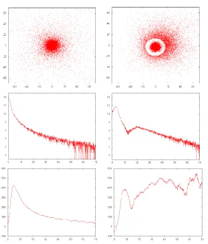
_added is reached, after 750 revolutions. Therefore at this time the full equations (19) are finally computed. Figure 2 shows the results. For comparison, figure11 shows exactly the same initial galaxy, after the same number of revolutions, but always simulating Newton’s law. The galactic center

shows the apparition of a ring [22]. This is discussed below. Newtonian logarithmic matter density profile is curved positively, from

0

to

50 kpc



galactocentric distances. But SMT one is a straight line between

20

and

70 kpc



. This is more compatible with experimental data. But of course, below

20 kpc



, the curve is no longer a straight line due to the existence of the ring. Radial and tangential speed dispersions are 2 or 3 times worse than

the one obtained with Newton’s law.

No stable spiral arms are noticed, like in [20]. Like in [20], they can appear only from time to time and are not stable structures. But the kind of apparition of arms shown by figure 4 seems to be provoked by the overall increase of

C

SMT though the whole galaxy. A

Kepler-like speed profile is of course shown under Newton’s law (figure 1). Those speed profiles are completely ruled out by experimental data, as commonly accepted. But SMT speed

profiles are much closer to flat curves. Of course this comes from the “smoothing” behavior

of SMT model, on velocities:

C

SMT increases with distance from the galactic center, due to matter density decrease. The galaxy speed profile of figure 2 has a shape which can be easily compared to the Milky-Way speed profile shape, for example. The speed profiles yielded by SMT are always far closer to experimental ones than those yielded by Newton’s

law. This was true for each executed simulation, which were done using various values of SMT parameters (an

NbP

_added different value, and also other constants than

7 / 39

,

40

,

39

). The values of those parameters in equations (19) are predicted by SMT but are not the most appropriate in order to yield the best profiles when comparing to experimental data. Nevertheless in this document, the simulations are always computing equations (19), except when expressly mentioned. Assuming different values for the parameters than those in equations (19), an almost perfectly flat speed profile can be obtained, for giant galaxies. This is also very much compatible with experimental data. Indeed, such a flat profile is observed in the case of UGC 2885 [23], NGC 801, or NGC 2403, for instance. Assuming

different values for the parameters a typical “increasing bell shape” profile can also be

obtained, for smaller galaxies. This is obtained in particular when the ring is weak, or

absent. Finally, a little “wave” is often noticed at the beginning of the speed profiles, which

is often present in experimental speed profiles. For example, on figure 2 this wave is located around

10 kpc



from the galactic center.

Galaxy stability is increased in lower density environments for medium- or large-sized galaxies. Indeed, it has been supposed when calculating equations (19), that IGM matter density is equal to



IGM

 

7



u0. But supposing



IGM



0

implies a modification of equations (19), such as

NbP

m



max



NbP

, 7 / 39





NbP

added



is replaced by

m

multiplication of gravitational forces by a factor of

8

, valid only when located out of the galaxy (or at the edge of it) will of course increase its stability. This has been confirmed by simulations (under the

h h



₀ hypothesis) and might be in accordance with experimental data [24]. In this



IGM



0

case, after its slow dissolution, a giant galaxy yields a very faint large galaxy, which can be easily compared with a LSB galaxy. But this does not occur under the



IGM

 

7



u₀ supposition, in which case this galaxy is only dissolving faster, without any remaining structure.

The computational flexibility is low and the liberty degrees are in the galaxy characteristics input. The first characteristic is the simulated matter density with respect to



0, in other

words

NbP

with respect to

NbP

0 . This depends on parameters such as the width and

volume matter density in a galaxy, with respect to its size. The second characteristic is the exact knowledge of gas and star distribution in the galaxies. This gas distribution was not taken into account in those simulations. Hopefully, in spiral galaxies the gas density is only a few percent of that of stars, and in elliptical galaxies it is even lower. Therefore this error might have no strong effects. But this might not be true for simulating a standalone dwarf galaxy. Anyhow this gas behavior simulation would require a specific kind of computation. The issue of this chapter is the most difficult and delicate. It would need a huge amount of work. But even without such a workload, here the SMT results speak for themselves.

6.6 Dwarf galaxies

The simulations show an occasional generation of dwarf galaxies, orbiting around the main galaxy. But this occurs only when simulating under SMT model. When simulating

Newton’s law, no dwarf galaxies were noticed. Dwarf galaxies are almost systematically

generated during the burst which occurs at the start of the simulation, when SMT model is immediately fully calculated, without beginning with a first phase in which Newton’s law is

active. Dwarf galaxies may also be generated with a simulation using a progressive installation of SMT model calculation. In this case, they can appear just at the beginning of the second phase of the simulation, which is executing progressively SMT model.

A faint galaxy, because it is faint, is probably located in a low or very low matter density environment. Therefore,

C

SMT is strong and the perceived gravitational attraction is high

(may be up to 40 times greater than Newton’s law attraction). As a result, the existence of this faint dwarf is more understandable under SMT than under Newton’s law, as well as its

important velocity in its revolution around a main galaxy. In front of this, faint and ultra-faint galaxies existence could be an issue under MOND theory [25]. The same mechanism

might explain the mystery of “the lower the surface brightness of a system, the larger its mass discrepancy [26]”. Indeed, low surface brightness galaxies are mainly isolated field galaxies. As such, they might also be located in a low matter density environment.

Those dwarf galaxies 2D generations are in accordance with experimental data. Indeed, studies of M31 [27], of the Milky-Way [28], and even of globular clusters and streams around the Milky-Way [28] has shown a systematic preferred location of dwarf galaxies along a common disk. Of course, it would be better to simulate in 3D, but the existence of 2D generations itself might be a result since no such dwarf galaxies were generated by the same simulations under Newton’s law. After a while they often dissolved progressively by

multiplication of gravitational forces by a factor of

8

, valid only when located out of the galaxy (or at the edge of it) will of course increase its stability. This has been confirmed by simulations (under the

h h



₀ hypothesis) and might be in accordance with experimental data [24]. In this



IGM



0

case, after its slow dissolution, a giant galaxy yields a very faint large galaxy, which can be easily compared with a LSB galaxy. But this does not occur under the



IGM

 

7



u₀ supposition, in which case this galaxy is only dissolving faster, without any remaining structure.

The computational flexibility is low and the liberty degrees are in the galaxy characteristics input. The first characteristic is the simulated matter density with respect to



0, in other

words

NbP

with respect to

NbP

0 . This depends on parameters such as the width and

volume matter density in a galaxy, with respect to its size. The second characteristic is the exact knowledge of gas and star distribution in the galaxies. This gas distribution was not taken into account in those simulations. Hopefully, in spiral galaxies the gas density is only a few percent of that of stars, and in elliptical galaxies it is even lower. Therefore this error might have no strong effects. But this might not be true for simulating a standalone dwarf galaxy. Anyhow this gas behavior simulation would require a specific kind of computation. The issue of this chapter is the most difficult and delicate. It would need a huge amount of work. But even without such a workload, here the SMT results speak for themselves.

6.6 Dwarf galaxies

The simulations show an occasional generation of dwarf galaxies, orbiting around the main galaxy. But this occurs only when simulating under SMT model. When simulating

Newton’s law, no dwarf galaxies were noticed. Dwarf galaxies are almost systematically

generated during the burst which occurs at the start of the simulation, when SMT model is immediately fully calculated, without beginning with a first phase in which Newton’s law is

active. Dwarf galaxies may also be generated with a simulation using a progressive installation of SMT model calculation. In this case, they can appear just at the beginning of the second phase of the simulation, which is executing progressively SMT model.

A faint galaxy, because it is faint, is probably located in a low or very low matter density environment. Therefore,

C

SMT is strong and the perceived gravitational attraction is high

(may be up to 40 times greater than Newton’s law attraction). As a result, the existence of this faint dwarf is more understandable under SMT than under Newton’s law, as well as its

important velocity in its revolution around a main galaxy. In front of this, faint and ultra-faint galaxies existence could be an issue under MOND theory [25]. The same mechanism

might explain the mystery of “the lower the surface brightness of a system, the larger its mass discrepancy [26]”. Indeed, low surface brightness galaxies are mainly isolated field galaxies. As such, they might also be located in a low matter density environment.

Those dwarf galaxies 2D generations are in accordance with experimental data. Indeed, studies of M31 [27], of the Milky-Way [28], and even of globular clusters and streams around the Milky-Way [28] has shown a systematic preferred location of dwarf galaxies along a common disk. Of course, it would be better to simulate in 3D, but the existence of 2D generations itself might be a result since no such dwarf galaxies were generated by the same simulations under Newton’s law. After a while they often dissolved progressively by

themselves. When the main galaxy contains a ring, those dwarf orbiting galaxies are generated only outside of this ring, therefore at more than

15 kpc



from the galactic center.

Figure 1: On the left are shown the results of a simulation executed under Newton’s law. The simulated galaxy is the same as in [20] after 750 revolutions, except that the galaxy mass is equal to

12

10

 sun masses, the initial galaxy ray is equal to



kpc.

10

5stars has been simulated in a 256 x 256 grid calculation over a 67 x 67 kpc² square. On top the 2D localization of the stars is drawn. In the middle 8 + log(ρ) is drawn, where ρ is the mean value over 13 kpc of galactic surface matter density. ρ unit is kg/m². On the bottom the tangential speed of the stars in km/s is drawn. For those three drawings, horizontal values (and vertical values for the top drawing) are galactocentric distances, with unit in kpc,

It was noticed also that they are often encountering the galactic center along their trajectory. But when this center contains a ring, which is often the case, they cannot dissolve themselves into it. They are systematically bouncing on the ring edge, forbidding any merge. This might result in a better stability of dwarf galaxies, with SMT, than with

Newton’s law.

By other means, the location of the Milky-Way on the plane containing the dwarf orbiting galaxies around M31 [27] is not explained by the model and would need a 3D simulation.

6.7 Ring galaxies

During the simulations a surprising result was found. Ring galaxies are oftenly generated by the SMT dynamic itself, without the help of any particular external event. They appear to be self-generated and stable structures. There is no longer the need to imagine any collision scenario between galaxies in order to explain their existence. And this is in

complete accordance with experimental data. For instance, in a region called “the general

field galaxy population lying behind the Tucana dwarf galaxy” [29], an “unexpectedly large number of ring galaxies” is found. This number is inconsistent with the hypothesis of ring galaxies generated only by collision. SMT might predict this abundance directly, without

supposing any “steeply increasing galaxy interaction rate with red-shift” [30]. Also, it could be difficult to understand why those ring galaxies are so young [31]. But this mean age of

1Gyr



might be understood by the simulations. Indeed, several dislocations of rings were noticed during the simulations. Those dislocations were always very quick and resulted in the same galaxy but without any more ring. This could indicate that nevertheless this stability is fragile, and therefore could explain this relatively young age. Even our

Milky-Way galaxy has been recently found to host a “ring of stars” [22].

When simulating a galaxy with the same characteristics (mass, star velocities, diameter) as the Milky-Way, this ring is found. It has a radius of 18 kpc



, which is exactly the experimentally observed ring radius. Also, the simulations has shown multi-ring stable structures. When simulating equations (19) they are noticed for big galaxies (having a ray greater than

50 kpc



). This is confirmed by experimental data. For example NGC 2859 double ring is obvious. The simulated ring shows strong matter density values also beyond the ring itself. This is not consistent with the visible rings of observational data. But as explained in [32], there is probably a low luminosity gaseous disk in ring galaxies.

The simulations seem to show that SMT prediction is the following. The width of the empty ring could not be greater than

r

_max. Moreover, it should be often below or just below this value. The simulations, for example the one of figure 3, shows a ring diameter of

34 kpc



, composed of a nucleus diameter of

10 kpc



, and an empty ring width of

12 kpc



(just below

r

max value). Those dimensions are similar to the Cartwheel galaxy dimensions,

It was noticed also that they are often encountering the galactic center along their trajectory. But when this center contains a ring, which is often the case, they cannot dissolve themselves into it. They are systematically bouncing on the ring edge, forbidding any merge. This might result in a better stability of dwarf galaxies, with SMT, than with

Newton’s law.

By other means, the location of the Milky-Way on the plane containing the dwarf orbiting galaxies around M31 [27] is not explained by the model and would need a 3D simulation.

6.7 Ring galaxies

During the simulations a surprising result was found. Ring galaxies are oftenly generated by the SMT dynamic itself, without the help of any particular external event. They appear to be self-generated and stable structures. There is no longer the need to imagine any collision scenario between galaxies in order to explain their existence. And this is in

complete accordance with experimental data. For instance, in a region called “the general

field galaxy population lying behind the Tucana dwarf galaxy” [29], an “unexpectedly large number of ring galaxies” is found. This number is inconsistent with the hypothesis of ring galaxies generated only by collision. SMT might predict this abundance directly, without

supposing any “steeply increasing galaxy interaction rate with red-shift” [30]. Also, it could be difficult to understand why those ring galaxies are so young [31]. But this mean age of

1Gyr



might be understood by the simulations. Indeed, several dislocations of rings were noticed during the simulations. Those dislocations were always very quick and resulted in the same galaxy but without any more ring. This could indicate that nevertheless this stability is fragile, and therefore could explain this relatively young age. Even our

Milky-Way galaxy has been recently found to host a “ring of stars” [22].

When simulating a galaxy with the same characteristics (mass, star velocities, diameter) as the Milky-Way, this ring is found. It has a radius of 18 kpc



, which is exactly the experimentally observed ring radius. Also, the simulations has shown multi-ring stable structures. When simulating equations (19) they are noticed for big galaxies (having a ray greater than

50 kpc



). This is confirmed by experimental data. For example NGC 2859 double ring is obvious. The simulated ring shows strong matter density values also beyond the ring itself. This is not consistent with the visible rings of observational data. But as explained in [32], there is probably a low luminosity gaseous disk in ring galaxies.

The simulations seem to show that SMT prediction is the following. The width of the empty ring could not be greater than

r

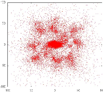
_max. Moreover, it should be often below or just below this value. The simulations, for example the one of figure 3, shows a ring diameter of

34 kpc



, composed of a nucleus diameter of

10 kpc



, and an empty ring width of

12 kpc



(just below

r

max value). Those dimensions are similar to the Cartwheel galaxy dimensions,

for example.

Figure 3: A simulated ring galaxy

The galaxy simulations shows that the ring’s ray of the simulated galaxies, when they

contain a ring, is always just below

r

max. Therefore an attempt could be to retrieve on

existing galaxies the statistical distribution of such a ray.

The simulation has shown that the particular truncated shape of the observed bars in the galaxies, along with the particular enrolled shape of arms around it, can result from the existence of a ring in those galaxies. For instance, on figure 4 the length of the bar is roughly equal to

35 kpc



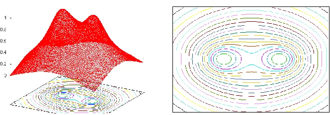
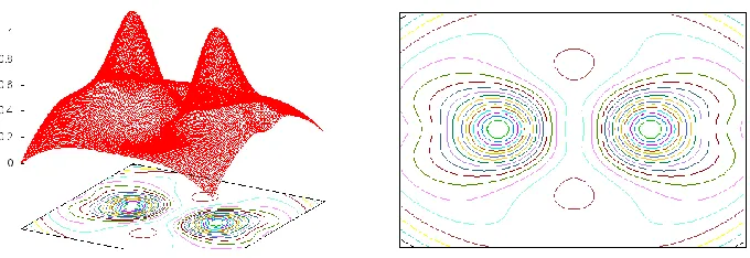
. This bar is the nucleus of an ancient ring galaxy. This nucleus started to deform itself and to rotate quickly. As a result the generated arms quickly enrolled around it. The result is then shown on the figure.

Figure 4: This galaxy shape appears when executing equations (20) with

705000

prog

NbP



,

NbP

_m



NbP

, and equations (20) with

h h



₀. At this time

prog

NbP

is decreasing at a pace of 15600 per galactic revolution. The central bar is rotating quickly, enrolling 2 arms around it. The simulated galaxy has a mass equal to

14

1.510



sun masses, and an initial ray equal to 1.9 kpc,

The similarity with observations is noticeable. And this was not obtained when simulating

Newton’s law with the same program. With Newton’s law, the bar and its arms always showed a “slow S”, as in [19]. This particular observed shape described above was never

noticeable neither for the bar nor for the arms, under Newton’s law.

Finally another weird prediction of the simulations is that the rotational speed of the stars located in the nucleus is sometimes opposite to the speed of the stars located outside of the ring. This prediction is validated by NGC 7217 speed profile.