Modified global k-means algorithm for minimum
sum-of-squares clustering problems
Adil M. Bagirov
Centre for Informatics and Applied Optimization, School of Information Technology and Mathematical Sciences, University of Ballarat, Victoria, 3353, Australia,
E-mail: [email protected], Tel.: +61 3 5327 9330, Fax: +61 3 5327 9289 Abstract
k-means algorithm and its variations are known to be fast clustering algorithms. However, they are sensitive to the choice of starting points and inefficient for solv-ing clustersolv-ing problems in large data sets. Recently, a new version of the k-means algorithm, the global k-means algorithm has been developed. It is an incremental algorithm that dynamically adds one cluster center at a time and uses each data point as a candidate for thek-th cluster center. Results of numerical experiments show that the globalk-means algorithm considerably outperforms thek-means algorithms. In this paper, a new version of the global k-means algorithm is proposed. A starting point for thek-th cluster center in this algorithm is computed by minimizing an aux-iliary cluster function. Results of numerical experiments on 14 data sets demonstrate the superiority of the new algorithm, however, it requires more computational time than the globalk-means algorithm.
Keywords: minimum sum-of-squares clustering, nonsmooth optimization, k-means algo-rithm, globalk-means algorithm.
1
Introduction
The cluster analysis deals with the problems of organization of a collection of patterns into clusters based on similarity. It is also known as theunsupervisedclassification of patterns and has found many applications in different areas.
In cluster analysis we assume that we have been given a finite set of points A in the
n-dimensional space IRn, that is
A={a1, . . . , am}, where ai ∈IRn, i= 1, . . . , m.
There are different types of clustering. In this paper, we consider the hard unconstrained partition clustering problem, that is the distribution of the points of the setAinto a given numberkof disjoint subsetsAj, j= 1, . . . , kwith respect to predefined criteria such that:
1) Aj 6=∅, j = 1, . . . , k;
2) AjT
3) A=
k
S
j=1 Aj;
4) no constraints are imposed on the clustersAj, j = 1, . . . , k.
The sets Aj, j = 1, . . . , k are called clusters. We assume that each cluster Aj can be identified by its center (or centroid) xj ∈IRn, j = 1, . . . , k. Then the clustering problem can be reduced to the following optimization problem (see [5, 22]):
minimize ψk(x, w) = 1 m m X i=1 k X j=1 wijkxj −aik2 (1) subject to x= (x1, . . . , xk)∈IRn×k, (2) k X j=1 wij = 1, i= 1, . . . , m, (3) and wij = 0 or 1, i= 1, . . . , m, j= 1, . . . , k (4)
wherewij is the association weight of pattern ai with the clusterj, given by
wij =
1 if pattern ai is allocated to the clusterj,
0 otherwise (5) and xj = Pm i=1wijai Pm i=1wij , j = 1, . . . , k. (6)
Herek · kis an Euclidean norm andwis anm×kmatrix. The problem (1) is also known as minimum sum-of-squares clustering problem.
Different algorithms have been proposed to solve the clustering problem. The paper [16] provides survey of most of existing algorithms. We mention among them heuristics likek-means algorithms and their variations (h-means, j-means etc.), mathematical pro-gramming techniques including dynamic propro-gramming, branch and bound, cutting plane, interior point methods, the variable neighborhood search algorithm and metaheuristics like simulated annealing, tabu search, genetic algorithms (see [1, 6, 7, 8, 9, 11, 12, 13, 14, 17, 21, 22, 23]).
The objective functionψkin (1) has many local minimizers (local solutions of problem
(1)-(6)). Local minimizers are points, where the function ψk achieves its smallest value
in some feasible neighborhood of these points. Global minimizers (or global solutions of problem (1)-(6)) ofψkare points where the function attains its least value over the feasible
set. It is expected that global minimzers provide better cluster structure of a data set. However, the most of clustering algorithms can locate only local minimizers of the function
ψk and these local minimizers may differ from global ones significantly as the number of
clusters increases. Global optimization algorithms, mentioned above, are not applicable to even relatively large data sets. Another difficulty is that the number of clusters is not known a priori.
Over the last several years different incremental algorithms have been proposed to address these difficulties. Incremental clustering algorithms attempt to optimally add one new cluster center at each stage. In order to compute k-partition of the set A these algorithms start from an initial state with thek−1 centers for the (k−1)-clustering problem and the remainingk-th center is placed in an appropriate position. Results of numerical experiments show that these algorithms are able to locate either a global minimizer or a local minimizer close to global one. The paper [4] develops an incremental algorithm based on nonsmooth optimization approach to clustering. The incremental approach is also discussed in [15].
The globalk-means algorithm, introduced in [18], is a significant improvement of the
k-means algorithm. It is an incremental algorithm. In this algorithm each data point is used as a starting point for the k-th cluster center. Such an approach leads at least to a near global minimizer. However this approach is not efficient since it is very time consuming, asmapplications ofk-means algorithm are made. Instead the authors suggest two procedures to reduce computational load.
The first algorithm is called the fast global k-means algorithm. Given the solu-tion x1, . . . , xk−1 of the (k−1)-clustering problem and the corresponding value ψ∗k−1 =
ψk−1(x1, . . . , xk−1) of the function ψk in (1) this algorithm does not execute thek-means
algorithm for each data point. Instead it computes an upper bound ψk∗ ≤ψk∗−1−bj on
theψ∗k, where bj = m X i=1 max{0, dik−1− kaj −aik2}, j = 1, . . . , m. (7)
Here dik−1 is the squared distance between ai and the closest center amongk−1 cluster centersx1, . . . , xk−1:
dik−1 = min
n
kx1−aik2, . . . ,kxk−1−aik2o. (8)
A data point aj ∈A with the maximum value of bj is chosen as a starting point for the
k-th cluster center.
In the second procedure a k−dtree is used to partitionAintom0m subsets; their centroids are used as starting points in the globalk-means scheme. The second procedure can be applied to low dimensional data sets.
In this paper, we propose a new version of the globalk-means algorithm. The difference between the new version and the fast globalk-means algorithm lies in the way a starting point for thek-th cluster center is obtained. Given the solutionx1, . . . , xk−1 of the (k− 1)-clustering problem, we formulate the so-called auxiliary cluster function:
¯ fk(y) = 1 m m X i=1 minndik−1,ky−aik2o. (9)
We apply the k-means algorithm to minimize this function. A local minimizer found is selected as a starting point for the k-th cluster center. We present the results of numer-ical experiments on 14 data sets. These results demonstrate that the superiority of the
proposed algorithm over the globalk-means algorithm, however, it is less computationally efficient.
The rest part of the paper is organized as follows: Section 2 gives a brief description of k-means and the global k-means algorithms. The nonsmooth optimization approach to clustering and an algorithm for the computation of a starting point is described in Section 3. Section 4 presents an algorithm for solving clustering problems. The results of numerical experiments are given in Section 5. Section 6 concludes the paper.
2
k
-means and the global
k
-means algorithms
In this section we give a brief description of thek-means and the globalk-means algorithms. The k-means algorithm proceeds as follows.
Algorithm 1 The k-means algorithm
Step 1. Choose a seed solution consisting ofkcenters (not necessarily belonging to A).
Step 2. Allocate data pointsa∈A to its closest center and obtaink-partition of A.
Step 3. Recompute centers for this new partition and go to Step 2 until no more data points change their clusters.
This algorithm is very sensitive to the choice of a starting point. It converges to a local solution which can significantly differ from the global solution in many large data sets.
The globalk-means algorithm proposed in [18] is an incremental clustering algorithm. To computek≤m clusters this algorithm proceeds as follows.
Algorithm 2 The global k-means algorithm.
Step 1. (Initialization) Compute the centroid x1 of the setA:
x1= 1 m m X i=1 ai, ai ∈A, i= 1, . . . , m (10) and setq= 1.
Step 2. (Stopping criterion) Setq =q+ 1. Ifq > k, then stop.
Step 3. Take the centers x1, x2, . . . , xq−1 from the previous iteration and consider each pointaofAas a starting point for theq-th cluster center, thus obtainingminitial solutions withqpoints (x1, . . . , xq−1, a); apply thek-means algorithm to each of them; keep the best
q-partition obtained and its centersy1, y2, . . . , yq.
This version of the algorithm is not applicable for clustering on middle sized and large data sets. Two procedures were introduced to reduce its complexity (see [18]). We mention here only one of them, because the second procedure is applicable only to low dimensional data sets. Let dik−1 be a squared distance betweenai ∈A, i = 1, . . . , m and the closest cluster center among thek−1 cluster centers obtained so far. In order to find the starting point for the k-th cluster center, for eachaj ∈A, j= 1, . . . , mwe compute bj using (7).
bj, j= 1, ..., mshows how much one can decrease the value of the functionψkfrom (1)
if the data pointaj is chosen as thek-th cluster center. Obviously, ifaj ∈A, j= 1, . . . , m
is not among the cluster centers x1, . . . , xk−1, then bj >0. This means that by selecting
any such data point as a starting point for the k-th cluster center one can decrease the value of the functionψkat least bybj. It is clear that a data pointaj ∈Awith the largest
value of the bj is the best candidate to be a starting point for the k-th cluster center.
Therefore, first we compute
¯b= max
j=1,...,mbj (11)
and find the data point aj ∈A such thatbj = ¯b. This data point is selected as a starting
point for the k-th cluster center. In our numerical experiments we use this procedure.
3
Computation of starting points
The clustering problem (1) can be reformulated in terms of nonsmooth, nonconvex opti-mization as follows (see [2, 3, 5]):
minimize fk(x) subject tox= (x1, . . . , xk)∈IRn×k, (12) where fk(x1, . . . , xk) = 1 m m X i=1 min j=1,...,kkx j−aik2. (13)
We callfk a cluster function. Comparing two different formulations (1) and (12) of the
hard clustering problem one can note that:
1. The objective function ψk depends on variables wij, i = 1, . . . , m, j = 1, . . . , k
(coefficients, which are integers) and x1, x2, . . . , xk, xj ∈IRn, j = 1, . . . , k (cluster centers, which are continuous variables). However, the functionfk depends only on
continuous variablesx1, . . . , xk.
2. The number of variables in problem (1) is (m+n)×kwhereas in problem (12) this number is only n×k and the number of variables does not depend on the number of instances. It should be noted that in many real-world data sets the number of instancesm is substantially greater than the number of featuresn.
3. The function ψk is continuously differentiable with respect to both variablesw and
x. Since the functionfkis represented as a sum of minima functions it is nonsmooth
4. Both functionsψk andfk are nonconvex.
5. Problem (1) is mixed integer nonlinear programming problem and problem (12) is nonsmooth global optimization problem. However, they are equivalent in the sense that their global minimizers coincide (see [5]).
Circumstances mentioned in Items 1 and 2 can be considered as advantages of the nonsmooth optimization formulation (12) of the clustering problem.
Assume that k >1 and the cluster centersx1, . . . , xk−1 for (k−1)-partition problem are known. Consideringk-partition problem we introduce the following function:
¯ fk(y) = 1 m m X i=1 minndik−1,ky−aik2 o , (14)
wherey∈IRnstands for k-th cluster center anddik−1 is defined in (8). The function ¯fkis
called anauxiliary cluster function. It depends on nvariables only. It is clear that
¯
fk(y) =fk(x1, . . . , xk−1, y) (15)
for all y ∈ IRn. This means that the auxiliary cluster function ¯fk coincides with the
cluster function fk with fixed k−1 cluster centers x1, . . . , xk−1. For each data point
ai ∈A consider also the following function:
ϕik(y) = min
n
dik−1,ky−aik2o. (16)
This function is represented as a minimum of constant and very simple quadratic function. If the data pointai is a cluster center then dik−1= 0 and ϕik(y)≡0. Otherwise
ϕik(y) = ky−aik2 ifky−aik2 < di k−1, dik−1 ifky−aik2 ≥di k−1. (17)
Since it is natural to assume that k < m, it is obvious that ϕik(y) >0 for some ai ∈A
andy∈IRn and ¯fk(y)>0 for ally∈IRn. As a minimum function, ϕik is nonsmooth and
nonconvex. It is nondifferentiable at pointsy ∈IRn, where ky−aik2 =di
k−1. Therefore,
the function ¯fk is also nonsmooth and nonconvex. The set where this function is
nondif-ferentiable can be represented as a union of sets, where functionsϕik are nondifferentiable.
Minimum value fk∗−1 of the function fk−1 is
fk∗−1= 1 m m X i=1 dik−1. (18)
If the data pointaj ∈A is not a cluster center, then
fk(x1, . . . , xk−1, aj) = 1 m m X i=1 minndik−1,kaj −aik2 o . (19)
Givenaj ∈A consider the following two index sets: I1= n i∈ {1, . . . , m}: kai−ajk2 ≥dik−1o, (20) I2= n i∈ {1, . . . , m}: kai−ajk2 < dik−1 o . (21)
Using this notation one can rewrite a formulae for bj from (7) as follows
bj = X i∈I2 dik−1− kaj−aik2 . (22) Then ¯ fk(aj) = fk(x1, . . . , xk−1, aj) = 1 m X i∈I1 dik−1+ X i∈I2 kaj−aik2 (23) and therefore, fk−1(x1, . . . , xk−1)−fk(x1, . . . , xk−1, aj) = X i∈I2 dik−1− kaj−aik2 = bj. (24)
This means that if one selectsaj as a starting point for the k-th cluster center then the optimal value of the function fk−1 can be decreased by bj ≥ 0. Therefore it is natural
to select a data point with the largest value ofbj as a starting point for the k-th cluster
center, which is done in one of the versions of the globalk-means algorithm. In this paper, we suggest to minimize the auxiliary cluster function ¯fk to find a starting point for the
k-th cluster center. Since the auxiliary cluster function coincides with the cluster function
fk when previous k−1 cluster centers x1, . . . , xk−1 are fixed, the minimization of the
auxiliary cluster function is equivalent to the minimization of the cluster functionfk with
fixedk−1 cluster centersx1, . . . , xk−1. The k-means algorithm is applied to find a local minimizer of ¯fk.
Now consider the set
D=ny∈IRn:ky−aik2≥dik−1o. (25)
¯
Dis the set where the distance between any its point y and any data point ai ∈A is no less than the distance between this data point and its cluster center. We also consider the following set D0 = IRn\D≡ n y∈IRn:∃I ⊂ {1, . . . , m}, I 6=∅:ky−aik< dik−1 ∀i∈I o . (26)
The function ¯fk is a constant on the setD and its value is
¯ fk(y) =d0 ≡ 1 m m X i=1 dik−1, ∀y∈D. (27)
It is clear thatxj ∈D for all j = 1, . . . , k−1 and ai ∈ D0 for all ai ∈A, ai 6=xj, j =
1, . . . , k−1. It is also clear that ¯fk(y)< d0 for all y∈D0.
Anyy∈D0can be selected as a starting point for thek-th cluster center. The function
¯
fkis nonconvex function with many local minima and the global minimizer of this function
can be the best candidate to be starting point for thek-th cluster center. However, it is not always possible to find the global minimizer of ¯fk in a reasonable time. Therefore, we
propose an algorithm for finding a local minimizer of the function ¯fk.
For anyy ∈D0 consider the following sets:
S1(y) = n ai ∈A:ky−aik2=dik−1 o , (28) S2(y) = n ai ∈A:ky−aik2< dik−1 o , (29) S3(y) = n ai ∈A:ky−aik2> dik−1 o . (30)
The setS2(y)6=∅ for any y∈D0.
The following algorithm is proposed to find a starting point for thek-th cluster center.
Algorithm 3 An algorithm for finding a starting point.
Step 1. For each ai ∈D0TA compute the set S2(ai), its center ci and the value ¯fk,ai = ¯
fk(ci) of the function ¯fk at the point ci.
Step 2. Compute ¯ fk,min= min ai∈D 0TA ¯ fk,ai, (31) aj = arg minai∈D 0TA ¯ fk,ai, (32)
the corresponding centercj and the setS
2(cj).
Step 3. Recompute the setS2(cj) and its center until no more data points escape or return
to this cluster.
Let ¯x be a cluster center generated by Algorithm 3. Since we consider the hard clustering problem, that is each data point belongs to only one cluster, one can assume thatS1(¯x) =∅.
Proposition 1 The point x¯ is a local minimizer of the functionf¯k.
The proof can be found in Appendix.
4
An incremental clustering algorithm
Algorithm 4 An incremental algorithm for clustering problems.
Step 1. (Initialization). Select a tolerance ε >0. Compute the center x1 ∈IRn of the set
A. Letf1 be the corresponding value of the objective function (13). Set k= 1.
Step 2. (Computation of the next cluster center). Set k=k+ 1. Letx1, . . . , xk−1 be the
cluster centers for (k−1)-partition problem. Apply Algorithm 3 to find a starting point ¯
y∈IRnfor the k-th cluster center.
Step 3. (Refinement of all cluster centers). Select (x1, . . . , xk−1,y¯) as a new starting point, applyk-means algorithm to solvek-partition problem. Lety1, . . . , ykbe a solution to this problem andfk be the corresponding value of the objective function (13).
Step 4. (Stopping criterion). If
fk−1−fk
f1 < ε (33)
then stop, otherwise setxi=yi, i= 1, . . . , k and go to Step 2.
It is clear that fk≥0 for all k≥1 and the sequence {fk} is decreasing, that is,
fk+1≤fk for all k≥1.
This means that the stopping criterion in Step 4 will be satisfied after finite many iter-ations. Thus Algorithm 4 computes as many clusters as the data set A contains with respect to the toleranceε >0.
The choice of the toleranceε >0 is crucial for Algorithm 4. Large values ofεcan result in the appearance of large clusters whereas small values can produce artificial clusters. The recommended values forεare ε∈[0.01,0.1].
5
Results of numerical experiments
To verify the efficiency of the proposed algorithm numerical experiments with a number of real-world data sets have been carried out on a PC Pentium-4 with CPU 2.4 GHz and RAM 512 MB. 14 data sets have been used in numerical experiments. The brief description of the data sets is given in Table 1. The detailed description of German towns, Bavaria postal data sets can be found in [22], Fisher’s Iris Plant data set in [10], the traveling salesman problems TSPLIB1060 and TSPLIB3038 in [20] and all other data sets in [19].
We computed up to 10 clusters in data sets with no more than 150 instances, up to 50 clusters in data sets with the number of instances between 150 and 1000 and up to 100 clusters in data sets with more than 1000 instances. The multi-start k-means (MS k-means) and the global k-means algorithms (GKM) have been used in numerical experiments for comparison purpose. To findkclusters, 100 times k starting points were randomly chosen in the MS k-means algorithm for all data sets and starting points were data points. In the GKM and the modified globalk-means (MGKM) algorithms a distance matrixD= (dij)mi,j=1 of a data set was computed before the start of the algorithms. Here dij =kai−ajk2. This matrix was used by both algorithms to find starting points.
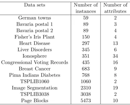
Table 1: The brief description of data sets
Data sets Number of Number of instances attributes
German towns 59 2
Bavaria postal 1 89 3 Bavaria postal 2 89 4 Fisher’s Iris Plant 150 4 Heart Disease 297 13 Liver Disorders 345 6
Ionosphere 351 34 Congressional Voting Records 435 16 Breast Cancer 683 9 Pima Indians Diabetes 768 8
TSPLIB1060 1060 2
Image Segmentation 2310 19
TSPLIB3038 3038 2
Page Blocks 5473 10
Results of numerical experiments are presented in Tables 2-8. In these tables we use the following notation:
• kis the number of clusters;
• fopt is the best known value of the cluster function (13) (multiplied by m) for the
corresponding number of clusters. For German towns, Bavaria Postal 1 and 2, Iris Plant data setsfoptis the value of the cluster function at the known global minimizer
( see [15]);
• E is the error in %;
• N is the number of Euclidean norm evaluations for the computation of the corre-sponding number of clusters. To avoid big numbers in tables we use its expression in the formN =α×10l and present the values ofαin tables. l= 4 for German towns, Bavaria Postal 1 and 2, Iris Plant data sets, l = 5 for Heart Disease, Liver Disor-ders, Ionosphere, Congressional Voting Records data sets, l= 6 for Breast Cancer, Pima Indians Diabetes, TSPLIB1060, Image Segmentation data sets andl = 7 for TSPLIB3038, Page Blocks data sets.
• tis the CPU time (in seconds).
The values of fopt for German towns, Bavaria postal , Iris Plant, Image Segmentation
(k ≤ 50), TSPLIB1060 (k ≤ 50) and TSPLIB3038 (k ≤ 50) data sets are available, for example, in [4, 15]. In all other cases we take asfopt the best value obtained by the MS
The error E is computed as
E= ( ¯f−fopt)
fopt
·100, (34)
where ¯f is the best value (multiplied bym) of the objective function (13) obtained by an algorithm. E = 0 implies that an algorithm finds the best known solution. We say that an algorithm finds a near global (or best known) solution if 0< E <1.
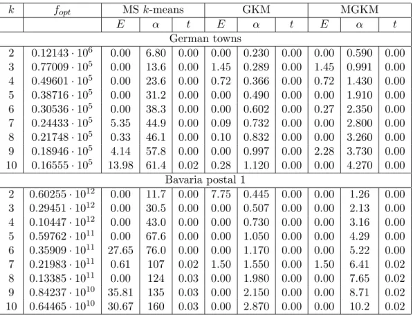
Table 2: Results for German towns and Bavaria postal 1 data sets
k fopt MSk-means GKM MGKM E α t E α t E α t German towns 2 0.12143·106 0.00 6.80 0.00 0.00 0.230 0.00 0.00 0.590 0.00 3 0.77009·105 0.00 13.6 0.00 1.45 0.289 0.00 1.45 0.991 0.00 4 0.49601·105 0.00 23.6 0.00 0.72 0.366 0.00 0.72 1.430 0.00 5 0.38716·105 0.00 31.2 0.00 0.00 0.490 0.00 0.00 1.910 0.00 6 0.30536·105 0.00 38.3 0.00 0.00 0.602 0.00 0.27 2.350 0.00 7 0.24433·105 5.35 44.9 0.00 0.09 0.732 0.00 0.00 2.800 0.00 8 0.21748·105 0.33 46.1 0.00 0.10 0.832 0.00 0.00 3.260 0.00 9 0.18946·105 4.14 57.8 0.00 0.00 0.997 0.00 2.28 3.730 0.00 10 0.16555·105 13.98 61.4 0.02 0.28 1.120 0.00 0.00 4.270 0.00 Bavaria postal 1 2 0.60255·1012 0.00 11.7 0.00 7.75 0.445 0.00 0.00 1.26 0.00 3 0.29451·1012 0.00 30.5 0.00 0.00 0.507 0.00 0.00 2.13 0.00 4 0.10447·1012 0.00 43.0 0.00 0.00 0.730 0.00 0.00 3.16 0.00 5 0.59762·1011 0.00 67.6 0.00 0.00 1.050 0.00 0.00 4.29 0.00 6 0.35909·1011 27.65 76.0 0.00 0.00 1.170 0.00 0.00 5.22 0.00 7 0.21983·1011 0.61 107 0.02 1.50 1.550 0.00 1.50 6.41 0.02 8 0.13385·1011 0.00 124 0.03 0.00 1.980 0.00 0.00 7.65 0.02 9 0.84237·1010 35.81 135 0.03 0.00 2.150 0.00 0.00 8.71 0.02 10 0.64465·1010 30.67 160 0.03 0.00 2.870 0.00 0.00 10.2 0.02
The results presented in Table 2 show that the MSk-means algorithm can locate global solutions when the number of clusters k ≤ 6 for German towns and k ≤ 5 for Bavaria postal 1 data sets. However, the results also show that this algorithm is not effective at computing more than 5 clusters even for small data sets. For German towns data set the GKM algorithm does as same as the MGKM algorithm four times, it does two times better and three times worse than the MGKM algorithm. For Bavaria postal 1 data set the GKM algorithm does as same as the MGKM algorithm eight times and it does once worse than the MGKM algorithm. The MS k-means algorithm is better than two other algorithms when the number of clusters k ≤ 5. The GKM algorithm requires less computational efforts than other two algorithms.
In these data sets both the GKM and MGKM algorithms in most of cases could locate either global or near global solutions. For German towns data set the MSk-means algorithm could find global or near global solutions six times, the GKM algorithm eight times and the MGKM algorithm seven times. On Bavaria Postal 1 data set the MS k -means algorithm finds global or near global solutions six times, the GKM algorithm seven times and the MGKM algorithm eight times.
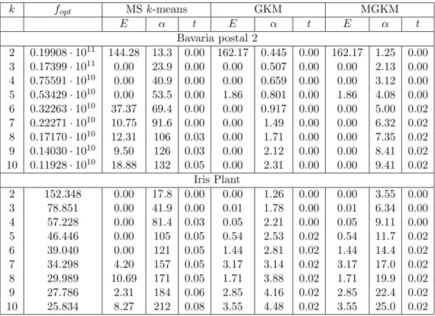
Table 3: Results for Bavaria postal 2 and Iris Plant data sets
k fopt MS k-means GKM MGKM E α t E α t E α t Bavaria postal 2 2 0.19908·1011 144.28 13.3 0.00 162.17 0.445 0.00 162.17 1.25 0.00 3 0.17399·1011 0.00 23.9 0.00 0.00 0.507 0.00 0.00 2.13 0.00 4 0.75591·1010 0.00 40.9 0.00 0.00 0.659 0.00 0.00 3.12 0.00 5 0.53429·1010 0.00 53.5 0.00 1.86 0.801 0.00 1.86 4.08 0.00 6 0.32263·1010 37.37 69.4 0.00 0.00 0.917 0.00 0.00 5.00 0.02 7 0.22271·1010 10.75 91.6 0.00 0.00 1.49 0.00 0.00 6.32 0.02 8 0.17170·1010 12.31 106 0.03 0.00 1.71 0.00 0.00 7.35 0.02 9 0.14030·1010 9.50 126 0.03 0.00 2.12 0.00 0.00 8.41 0.02 10 0.11928·1010 18.88 132 0.05 0.00 2.31 0.00 0.00 9.41 0.02 Iris Plant 2 152.348 0.00 17.8 0.00 0.00 1.26 0.00 0.00 3.55 0.00 3 78.851 0.00 41.9 0.00 0.01 1.78 0.00 0.01 6.34 0.00 4 57.228 0.00 81.4 0.03 0.05 2.21 0.00 0.05 9.11 0.00 5 46.446 0.00 105 0.05 0.54 2.53 0.02 0.54 11.7 0.02 6 39.040 0.00 121 0.05 1.44 2.81 0.02 1.44 14.4 0.02 7 34.298 4.20 157 0.05 3.17 3.14 0.02 3.17 17.0 0.02 8 29.989 10.69 171 0.05 1.71 3.88 0.02 1.71 19.9 0.02 9 27.786 2.31 184 0.06 2.85 4.16 0.02 2.85 22.4 0.02 10 25.834 8.27 212 0.08 3.55 4.48 0.02 3.55 25.0 0.02
As one can see from Table 3, the GKM and MGKM algorithms find the same solutions for both Bavaria postal 2 and Iris Plant data sets. However, the GKM algorithm requires less computational efforts than the MGKM algorithm.
All algorithms failed to find the global solution fork= 2 in Bavaria postal 2 data set. The MS k-means algorithm fails to find the global solution when the number of clusters
k >5 for Bavaria postal 2 data set andk >6 for Iris Plant data set. For Bavaria postal 2 data set the MS k-means algorithm finds global or near global solutions three times, the GKM and MGKM algorithms seven times. For Iris Plant data set the MS k-means algorithm finds such solutions five times, the GKM and MGKM algorithms four times.
The results from Table 4 demonstrate that the MS k-means algorithm cannot locate the global solution for Heart Disease data set when k > 5 and for Liver Disorders data
Table 4: Results for Heart Disease and Liver Disorders data sets k fopt MS k-means GKM MGKM E α t E α t E α t Heart Disease 2 0.59890·106 0.00 7.86 0.16 0.00 0.505 0.02 0.00 1.40 0.02 5 0.32797·106 0.00 29.7 0.47 0.52 0.722 0.02 0.52 4.25 0.05 10 0.20222·106 2.76 80.1 0.84 0.00 1.57 0.03 1.93 9.31 0.09 15 0.14771·106 8.79 113 1.14 0.00 2.68 0.06 0.68 14.6 0.17 20 0.11778·106 7.46 130 1.19 0.00 3.98 0.09 1.34 20.4 0.23 25 0.10213·106 5.16 151 1.31 0.48 5.46 0.11 0.00 25.9 0.33 30 0.88795·105 18.66 180 1.64 0.00 6.80 0.14 0.31 31.5 0.44 40 0.68645·105 28.65 213 1.67 1.71 9.71 0.20 0.00 43.5 0.69 50 0.55894·105 33.68 250 1.88 2.06 13.2 0.27 0.00 55.4 1.03 Liver Disorders 2 0.42398·106 0.00 6.91 0.09 93.96 0.600 0.00 93.96 0.600 0.00 5 0.21826·106 0.00 41.7 0.42 0.08 0.990 0.03 0.08 5.75 0.03 10 0.12768·106 0.09 87.5 0.67 0.00 2.00 0.05 0.02 12.7 0.08 15 0.97474·105 6.53 147 0.92 1.62 3.41 0.08 0.00 20.3 0.13 20 0.81820·105 9.05 184 1.11 0.29 5.12 0.11 0.00 27.5 0.19 25 0.70419·105 16.64 208 1.17 0.23 6.99 0.13 0.00 35.1 0.28 30 0.61143·105 24.33 229 1.31 0.21 8.75 0.16 0.00 43.0 0.39 40 0.47832·105 37.83 290 1.61 3.59 14.6 0.23 0.00 60.4 0.66 50 0.39581·105 50.64 337 1.88 5.50 19.9 0.28 0.00 78.0 0.97
set when k > 10. For Heart Disease data set the GKM algorithm does as same as the MGKM algorithm two times, it does four times better and three times worse than the MGKM algorithm. For Liver Disorder data set the GKM algorithm does as same as the MGKM algorithm two times and it does once better and six times worse than the MGKM algorithm. Again the GKM algorithm requires less computational efforts than other two algorithms.
For Heart Disease data set the MS k-means algorithm finds the best known or near best known solutions two times, the GKM and MGKM algorithms find those solutions seven times. For Liver Disorder data set the MSk-means algorithm finds the best known or near best known solutions three times, the GKM algorithm five times and the MGKM algorithm eight times. The MGKM algorithm outperforms two other algorithms as the number of clusters increases.
In Ionosphere and Congressional Voting Records data sets the MSk-means algorithm again cannot find the global solution when the number of clusters k > 5 (see Table 5). For Ionosphere data set the GKM algorithm does as same as the MGKM algorithm once, it does once better and seven times worse than the MGKM algorithm. For Congressional Voting Records data set the GKM algorithm does as same as the MGKM algorithm two
Table 5: Results for Ionosphere and Congressional Voting Records data sets k fopt MSk-means GKM MGKM E α t E α t E α t Ionosphere 2 0.24194·104 0.00 5.75 0.45 0.00 0.663 0.03 0.00 1.90 0.05 5 0.18915·104 0.00 26.2 0.70 0.07 0.899 0.05 0.18 5.85 0.13 10 0.15694·104 1.02 67.3 1.88 1.73 1.40 0.08 0.00 12.5 0.27 15 0.14014·104 3.72 104 2.47 4.31 1.88 0.11 0.00 19.3 0.42 20 0.12714·104 2.62 136 3.05 5.73 2.53 0.13 0.00 26.1 0.77 25 0.11486·104 11.95 182 4.02 6.76 3.35 0.16 0.00 33.3 1.39 30 0.10469·104 13.99 200 4.19 7.37 4.35 0.20 0.00 40.6 2.20 40 0.85658·103 30.35 273 5.59 7.82 7.88 0.30 0.00 55.8 4.77 50 0.70258·103 45.90 352 6.72 6.63 11.1 0.38 0.00 71.6 8.39
Congressional Voting Records
2 0.16409·104 0.00 7.77 0.28 0.12 1.00 0.02 0.12 2.91 0.03 5 0.13371·104 0.00 37.5 0.39 1.02 1.60 0.05 1.02 9.15 0.11 10 0.11312·104 1.12 95.8 1.48 1.33 2.84 0.08 0.00 19.7 0.20 15 0.10089·104 1.42 134 1.73 0.00 4.72 0.13 0.17 30.7 0.31 20 0.91445·103 6.11 174 2.30 1.40 6.25 0.17 0.00 41.9 0.44 25 0.85032·103 5.87 209 2.38 2.03 7.55 0.22 0.00 53.0 0.58 30 0.78216·103 12.31 238 2.73 2.73 10.1 0.27 0.00 64.8 0.73 40 0.69412·103 18.36 291 3.20 3.32 15.2 0.38 0.00 87.1 1.16 50 0.62451·103 25.72 351 3.69 4.35 19.9 0.48 0.00 111 1.84
times and it does once better and six times worse than the MGKM algorithm. Again the GKM algorithm requires less computational efforts than other two algorithms.
For Ionosphere data set the MSk-means and GKM algorithms find the best known (or near best known) solutions two times and MGKM algorithms finds those solutions nine times. For Congressional Voting Records data set the MSk-means and GKM algorithms find such solutions two times and the MGKM algorithm eight times. The MGKM algo-rithm significantly outperforms two other algoalgo-rithms as the number of clusters increases. Results from Table 6 show that the MS k-means algorithm cannot find the global solution when the number of clusters k >5 in Breast Cancer data set and when k > 10 in Pima Indians Diabetes data set. For Breast Cancer data set the GKM algorithm does as same as the MGKM algorithm once, it does two times better and six times worse than the MGKM algorithm. For Pima Indians Diabetes data set the GKM algorithm does as same as the MGKM algorithm three times and it does four times better and two times worse than the MGKM algorithm. Again the GKM algorithm requires less computational efforts than other two algorithms.
For Breast Cancer data set the MSk-means and GKM algorithms find the best known or near best known solutions three times and the MGKM algorithm finds such solutions
Table 6: Results for Breast Cancer and Pima Indians Diabetes data sets k fopt MSk-means GKM MGKM E α t E α t E α t Breast Cancer 2 0.19323·105 0.00 0.891 0.38 0.00 0.242 0.05 0.00 0.709 0.06 5 0.13705·105 0.00 8.50 1.30 2.28 0.306 0.09 1.86 2.17 0.17 10 0.10216·105 4.40 15.8 1.47 0.00 0.559 0.17 0.02 4.60 0.33 15 0.87813·104 0.20 24.2 1.91 0.00 0.803 0.23 0.04 7.14 0.48 20 0.77855·104 5.99 34.0 2.45 1.80 1.06 0.31 0.00 9.65 0.66 25 0.69682·104 9.87 40.6 2.66 4.12 1.27 0.38 0.00 12.4 0.83 30 0.64415·104 10.44 49.3 3.23 3.43 1.63 0.45 0.00 15.0 0.98 40 0.56171·104 15.99 61.7 3.77 3.70 2.22 0.61 0.00 20.2 1.39 50 0.49896·104 22.37 74.2 4.27 4.21 3.03 0.77 0.00 25.6 1.83
Pima Indians Diabetes
2 0.51424·107 0.00 2.30 1.13 0.00 0.318 0.06 0.00 0.909 0.09 5 0.17370·107 0.00 10.6 1.58 0.14 0.440 0.13 0.14 2.81 0.22 10 0.94436·106 0.00 30.4 2.75 0.36 0.646 0.20 0.36 5.98 0.41 15 0.69725·106 2.30 46.5 3.73 0.00 1.06 0.30 0.03 9.36 0.59 20 0.57438·106 3.50 56.1 3.94 0.00 1.53 0.39 0.36 12.8 0.80 25 0.49058·106 5.75 66.5 4.61 0.00 2.20 0.52 0.53 16.3 0.98 30 0.43641·106 10.65 77.2 5.28 1.84 2.53 0.59 0.00 19.9 1.22 40 0.36116·106 13.77 106 6.61 0.00 4.02 0.83 0.51 27.0 1.70 50 0.31439·106 20.16 120 7.09 0.24 5.31 1.06 0.00 34.1 2.28
eight times. For Pima Indians Diabetes data set the MS k-means algorithm finds such solutions three times, the GKM algorithm eight times and the MGKM algorithm nine times.
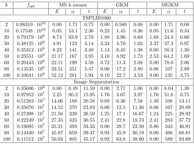
The MSk-means algorithm cannot find the global solution when the number of clusters
k > 10 for TSPLIB1060 data set and k > 2 for Image Segmentation data set (Table 7). For TSPLIB1060 data set the GKM algorithm does as same as the MGKM algorithm two times, it does two times better and five times worse than the MGKM algorithm. For Image Segmentation data set the GKM algorithm does as same as the MGKM algorithm five times and it does two times better and two times worse than the MGKM algorithm. Again the GKM algorithm requires less computational efforts than two other algorithms. For TSPLIB1060 data set the MS k-means algorithm finds the best known (or near best known) solutions two times, the GKM algorithm five times and the MGKM algorithm six times. For Image Segmentation data set the MSk-means algorithm finds such solutions only once, the GKM algorithm six times and the MGKM algorithm five times.
The MS k-means algorithm again cannot find the global solution when the number of clusters k > 10 for TSPLIB3038 data set and k ≥ 2 for Page Blocks data set (Table 8). For TSPLIB3038 data set the GKM algorithm does as same as the MGKM algorithm
Table 7: Results for TSPLIB1060 and Image Segmentation data sets k fopt MSk-means GKM MGKM E α t E α t E α t TSPLIB1060 2 0.98319·1010 0.00 1.71 0.75 0.00 0.580 0.08 0.00 1.71 0.08 10 0.17548·1010 0.05 53.1 2.36 0.23 1.45 0.36 0.05 11.6 0.34 20 0.79179·109 8.74 93.9 2.78 1.88 2.96 0.69 1.88 24.3 0.66 30 0.48125·109 4.91 123 3.14 3.34 4.70 1.03 3.37 37.3 0.97 40 0.35312·109 8.23 141 3.48 1.14 6.45 1.38 0.00 50.3 1.30 50 0.25551·109 21.17 167 3.95 3.10 8.92 1.73 2.53 64.2 1.69 60 0.20443·109 22.11 199 4.58 0.72 11.3 2.08 0.00 78.0 2.06 80 0.13535·109 33.51 251 5.47 0.00 17.2 2.80 0.06 107 2.89 100 0.10041·109 52.12 281 5.94 0.10 22.7 3.53 0.00 135 3.75 Image Segmentation 2 0.35606·108 0.00 6.49 11.59 0.00 2.71 1.06 0.00 8.04 1.39 10 0.97952·107 2.25 80.3 15.95 1.76 3.67 3.97 1.76 51.6 6.75 20 0.51283·107 14.06 188 20.58 0.09 6.36 7.58 1.49 108 13.11 30 0.35076·107 14.52 270 23.83 0.06 12.5 11.36 0.06 167 20.89 40 0.27398·107 21.56 339 26.59 1.25 17.1 16.67 1.24 225 28.92 50 0.22249·107 27.33 423 30.55 2.41 22.8 18.73 2.41 283 37.72 60 0.19095·107 35.21 493 33.33 0.00 29.7 22.50 0.86 343 46.91 80 0.14440·107 45.87 659 39.47 0.93 45.9 30.19 0.00 466 68.81 100 0.11512·107 50.03 805 45.17 0.92 63.8 38.00 0.00 589 93.69
two times, it does three times better and four times worse than the MGKM algorithm. For Page Blocks data set the GKM algorithm does three times better and six times worse than the MGKM algorithm. The MGKM algorithm requires less CPU time than other two algorithms for both data sets.
For TSPLIB3038 data set the MSk-means algorithm finds the best known (or near best known) solutions three times, the GKM algorithm four times and the MGKM algorithm seven times. For Block Pages data set the MSk-means algorithm finds such solutions only once, the GKM algorithm eight times and the MGKM algorithm nine times.
Overall on 14 data sets, the GKM algorithm does as same as the MGKM algorithm 50 (39.7 %) times, it does 25 (19.8 %) times better and 51 (40.5 %) times worse than the MGKM algorithm. The MS k-means algorithm finds the best known (or near best known) solutions 42 (33.3 %) times, the GKM algorithm 76 (60.3 %) times and the MGKM algorithm 102 (81.0 %) times.
The following results clearly demonstrate that the MGKM algorithm is better than two other algorithms at computing large number of clusters (k≥ 25) in larger data sets (m >150). Indeed, in this case the GKM algorithm does as same as the MGKM algorithm 3 (6.3 %) times, it does 12 (25.0 %) times better and 33 (68.7 %) times worse than the
Table 8: Results for TSPLIB3038 and Page Blocks data sets k fopt MS k-means GKM MGKM E α t E α t E α t TSPLIB3038 2 0.31688·1010 0.00 0.860 12.97 0.00 0.469 1.38 0.00 1.39 0.86 10 0.56025·109 0.00 14.2 11.52 2.78 0.857 8.41 0.58 9.16 3.30 20 0.26681·109 0.42 37.1 14.53 2.00 1.60 16.63 0.48 19.2 5.77 30 0.17557·109 1.16 57.8 19.09 1.45 2.97 25.00 0.67 29.5 8.25 40 0.12548·109 2.24 74.6 22.28 1.35 3.98 33.23 1.35 39.9 10.70 50 0.98400·108 2.60 84.5 23.55 1.19 5.26 41.52 1.41 50.5 13.23 60 0.82006·108 5.56 103 27.64 0.00 6.39 49.75 0.98 61.0 15.75 80 0.61217·108 4.84 119 30.02 0.00 9.56 66.42 0.63 82.9 20.94 100 0.48912·108 5.99 138 33.59 0.59 12.9 83.16 0.00 105 26.11 Page Blocks 2 0.57937·1011 0.24 1.82 577.05 0.24 1.50 8.19 0.00 4.50 6.92 10 0.45662·1010 206.38 42.3 168.45 0.80 1.66 49.62 0.00 28.6 34.09 20 0.17139·1010 70.44 259 367.39 0.00 2.30 92.30 0.19 59.3 62.09 30 0.94106·109 399.77 452 417.28 0.75 3.15 132.41 0.00 90.1 89.42 40 0.62570·109 485.89 641 477.88 0.17 4.22 172.13 0.00 121 118.55 50 0.42937·109 725.19 760 503.03 0.04 5.86 212.27 0.00 152 149.77 60 0.31185·109 1057.99 920 571.77 0.00 10.1 254.88 0.33 185 184.06 80 0.20576·109 1647.96 889 513.25 1.46 14.2 334.36 0.00 250 258.69 100 0.14545·109 998.80 796 443.64 0.00 20.5 415.19 0.10 316 346.94
MGKM algorithm. The MS k-means algorithm failed to find the best known (or near best known) solutions, the GKM algorithm finds such solutions 22 (45.8 %) times and the MGKM algorithm 42 (87.5 %) times.
Thus, these results allow us to draw the following conclusions:
1. The MS k-means algorithm is not effective at computing even moderately large number of clusters in large data sets.
2. Three algorithms, considered in this paper, are different versions of the k-means algorithm. Their main difference is in the way they compute starting points. In the MS k-means algorithm starting points are chosen randomly, however in two other algorithms special schemes are applied to find them. Results of numerical experi-ments show that the MGKM algorithm is more effective than two other algorithms at finding good starting points.
3. There is no any significant difference between the results of the GKM and MGKM algorithms on small data sets. However, the GKM requires significantly less
compu-tational efforts.
4. The MGKM algorithm works better than the GKM algorithm for large data sets and for large number of clusters (k≥25). The MGKM algorithm is especially effective for data sets such as Ionosphere, Congressional Voting Records, Liver Disorders data sets, which do not have well separated clusters.
6
Conclusions
In this paper, we have developed the new version of the global k-means algorithm, the modified globalk-means algorithm. This algorithm computes clusters incrementally and to computek-partition of a data set it usesk−1 cluster centers from the previous iteration. An important step in this algorithm is the computation of a starting point for the k -th cluster center. This starting point is computed by minimizing -the so-called auxiliary cluster function. The proposed algorithm computes as many clusters as a data set contains with respect to a given tolerance.
We have presented the results of numerical experiments on 14 data sets. These re-sults clearly demonstrate that the multi-start k-means algorithm cannot be alternative to both the global k-means and the modified global k-means algorithms when the num-ber of clusters k > 5. The results presented also demonstrate that the modified global
k-means algorithm is more effective than the global k-means algorithm at computing of large number of clusters in large data sets. However, the former algorithm requires more CPU time than the latter one. Results presented in this paper again confirms that the choice of starting points ink-means algorithms is crucial.
Acknowledgements
Dr. Adil Bagirov is the recipient of an Australian Research Council Australian Research Fellowship (Project number: DP 0666061).
The author thanks an anonymous referee for comments and criticism that significantly improved the quality of the paper.
References
[1] K.S. Al-Sultan, A tabu search approach to the clustering problem, Pattern Recogni-tion, 28(9)(1995) 1443-1451.
[2] A.M. Bagirov, A.M. Rubinov, J. Yearwood, A global optimisation approach to clas-sification, Optimization and Engineering, 3(2)(2002) 129-155.
[3] A.M. Bagirov, A.M. Rubinov, N.V. Soukhoroukova, J. Yearwood, Supervised and un-supervised data classification via nonsmooth and global optimization, TOP: Spanish Operations Research Journal, 11(1)(2003) 1-93.
[4] A.M. Bagirov, J. Yearwood, A new nonsmooth optimization algorithm for mini-mum sum-of-squares clustering problems, European Journal of Operational Research,
170(2006) 578-596.
[5] H.H. Bock, Clustering and neural networks, in: A. Rizzi, M. Vichi, H.H. Bock (eds),
Advances in Data Science and Classification, Springer-Verlag, Berlin, 1998, pp. 265-277.
[6] D.E. Brown, C.L. Entail, A practical application of simulated annealing to the clus-tering problem, Pattern Recognition, 25(1992) 401-412.
[7] O. du Merle, P. Hansen, B. Jaumard, N. Mladenovic, An interior point method for minimum sum-of-squares clustering, SIAM J. on Scientific Computing, 21(2001) 1485-1505.
[8] G. Diehr, Evaluation of a branch and bound algorithm for clustering, SIAM J. Sci-entific and Statistical Computing, 6(1985) 268-284.
[9] R. Dubes, A.K. Jain, Clustering techniques: the user’s dilemma,Pattern Recognition, 8(1976) 247-260.
[10] R.A. Fisher, The use of multiple measurements in taxonomic problems,Ann. Eugen-ics, VII part II (1936) 179-188. Reprinted in: Fisher R.A. Contributions to Mathe-matical Statistics, Wiley, 1950.
[11] P. Hanjoul, D. Peeters, A comparison of two dual-based procedures for solving the
p-median problem,European Journal of Operational Research,20(1985) 387-396.
[12] P. Hansen, B. Jaumard, Cluster analysis and mathematical programming, Mathemat-ical Programming, 79(1-3)(1997) 191-215.
[13] P. Hansen, N. Mladenovic, J-means: a new heuristic for minimum sum-of-squares clustering, Pattern Recognition, 4(2001) 405-413.
[14] P. Hansen, N. Mladenovic, Variable neighborhood decomposition search,Journal of Heuristic, 7(2001) 335-350.
[15] Hansen P., Ngai E., Cheung B.K., Mladenovic N. (2002) Analysis of globalk-means, an incremental heuristic for minimum sum-of-squares clustering, Les Cahiers du GERAD, G-2002-43, 2002. (to appear in: J. of Classification).
[16] A.K. Jain, M.N. Murty, P.J. Flynn, Data clustering: a review, ACM Computing Surveys,31(3)(1999) 264-323.
[17] W.L.G. Koontz, P.M. Narendra, K. Fukunaga, A branch and bound clustering algo-rithm,IEEE Transactions on Computers, 24(1975) 908-915.
[18] A. Likas, M. Vlassis, J. Verbeek, The global k-means clustering algorithm, Pattern Recognition, 36(2003) 451-461.
[19] UCI repository of machine learning databases, http://www.ics.uci.edu/mlearn/MLRepository.html.
[20] G. Reinelt, TSP-LIB-A Traveling Salesman Library,ORSA J. Comput.3(1991), 319-350.
[21] S.Z. Selim, K.S. Al-Sultan, A simulated annealing algorithm for the clustering, Pat-tern Recognition, 24(10)(1991) 1003-1008.
[22] H. Spath,Cluster Analysis Algorithms, Ellis Horwood Limited, Chichester, 1980.
[23] L.X. Sun, Y.L. Xie, X.H. Song, J.H. Wang, R.Q. Yu, Cluster analysis by simulated annealing, Computers and Chemistry,18(1994) 103-108.
7
Appendix
Proof of Proposition 1: SinceS1(¯x) =∅we get that
¯ fk(¯x) = 1 m X ai∈S 2(¯x) kx¯−aik2+ 1 m X ai∈S 3(¯x) dik−1. (35)
It is clear that ¯x is a global minimizer of the convex function
Φ(x) = 1 m X ai∈S 2(¯x) kx−aik2 (36)
that is Φ(¯x)≤Φ(x) for allx∈IRn.
LetBε(¯x) ={y∈IRn: ky−x¯k< ε}.There existsε >0 such that
kx−aik2< dik−1 ∀ai∈S2(¯x) and ∀ x∈Bε(¯x), (37)
kx−aik2> di
k−1 ∀ai∈S3(¯x) and ∀ x∈Bε(¯x). (38)
Then for anyx∈Bε(¯x) we have
¯ fk(x) = 1 m X ai∈S 2(¯x) kx−aik2+ 1 m X ai∈S 3(¯x) dik−1 = Φ(x) + 1 m X ai∈S 3(¯x) dik−1 ≥ Φ(¯x) + 1 m X ai∈S 3(¯x) dik−1 = f¯k(¯x). (39)