UNIVERSITY OF
CAMBRIDGE
Cambridge Working
Papers in Economics
Transformed Maximum Likelihood
Estimation of Short Dynamic
Panel Data Models with
Interactive Effects
Kazuhiko Hayakawa, Hashem Peseran
and Vanessa Smith
Transformed Maximum Likelihood Estimation of Short Dynamic
Panel Data Models with Interactive E¤ects
Kazuhiko Hayakawa Hiroshima University
M. Hashem Pesaran
USC and Trinity College, Cambridge
L. Vanessa Smith University of York May 2014
Abstract
This paper proposes the transformed maximum likelihood estimator for short dynamic panel data models with interactive …xed e¤ects, and provides an extension of Hsiao et al. (2002) that allows for a multifactor error structure. This is an important extension since it retains the advantages of the transformed likelihood approach, whilst at the same time allows for observed factors (…xed or random). Small sample results obtained from Monte Carlo simulations show that the transformed ML estimator performs well in …nite samples and outperforms the GMM estimators proposed in the literature in almost all cases considered.
JEL Classi…cations: C12, C13, C23
Keywords: shortT dynamic panels, transformed maximum likelihood, multi-factor error structure, interactive …xed e¤ects
The authors would like to thank Vasilis Sara…dis as well as participants at the conference on Cross-sectional Dependence in Panel Data Models, May 2013, Cambridge, for helpful comments on a preliminary version of the paper. Part of this paper was written whilst Hayakawa was visiting the University of Cambridge as a JSPS Postdoctoral Fellow for Research Abroad. He acknowledges …nancial support from the JSPS Fellowship and the Grant-in-Aid for Scienti…c Research (KAKENHI 22730178, 25780153) provided by the JSPS. Pesaran and Smith acknowledge …nancial support from the ESRC Grant No. ES/1031626/1.
1
Introduction
There now exists an extensive literature on the estimation of linear dynamic panel data models where the time dimension (T) is short and …xed relative to the cross section dimension (N), which is large. Such panels are usually referred to as micro panels, and often arise in microeconometric applications. For example, many empirical applications based on survey data such as the British Household Panel Surveys (BHPS) and the Panel Study in Income Dynamics (PSID) are character-ized by data covering relatively short time periods. Although it is now quite common to include dynamics in such studies, it is rare to …nd studies that allow for error cross section dependence as well. In most empirical applications time dummies are used to deal with cross section dependence, which is valid only if the time e¤ect is homogeneous over the cross section units. Short T panels also arise in the cross country empirical growth literature where data is typically averaged over …ve to seven years to eliminate the business cycle e¤ects. Both generalized method of moments (GMM) and likelihood approaches have been advanced to estimate such panel data models. See, for exam-ple, Anderson and Hsiao (1981), Arellano and Bond (1991), Arellano and Bover (1995), Blundell and Bond (1998), Hsiao et al. (2002) and Binder et al. (2005).1 However, this literature assumes that the errors are cross sectionally independent, which might not hold in many applications where cross section units are subject to common unobserved e¤ects, or possibly spatial or network spill-over e¤ects. Ignoring cross section dependence can have important consequences for conventional estimators of dynamic panels. Phillips and Sul (2007) study the impact of cross section dependence modelled as a factor structure on the inconsistency of the pooled least squares estimate of a short dynamic panel regression. Sara…dis and Robertson (2009) investigate the properties of a number of standard widely used generalized method of moments (GMM) estimators under cross section dependence and show that such estimators are inconsistent.
In applications where the spatial patterns are important and can be characterized by known spatial weight matrices, error cross section dependence is typically modelled as spatial autoregres-sions and estimated jointly with the other parameters of the dynamic panel data model. Lee and Yu (2010) provide a review. For smallT, Elhorst (2005) and Su and Yang (2007) consider random e¤ects as well as …xed e¤ects speci…cations. In the latter case they apply the …rst-di¤erencing operator to eliminate the …xed e¤ects and then use the transformed likelihood approach of Hsiao et al. (2002) to deal with the initial value problem. The treatment of the initial values in spatial dynamic panel data models poses additional di¢ culties and requires further investigation. More recently Jacobs et al. (2009) discuss GMM estimation of dynamic …xed e¤ect panel data models featuring spatially correlated errors and endogenous interaction.
However, in addition to the spatial e¤ects it is also likely that the error cross section dependence could be a result of omitted unobserved common factor(s). This class of models has been the subject of intensive research over the past …ve years and robust estimation procedures have been advanced in the case of panels whereN andT are both large.2 In contrast, little work has been done so far on the estimation of shortT dynamic panels where error cross section dependence is due to unobserved common factors. An early contribution by MaCurdy (1982) features panel models with an error structure that combines factor schemes with autoregressive-moving average models estimated by maximum likelihood and used to analyze the error process associated with the earnings of prime
1The analysis of Hsiao et al. (2002) is extended by Hayakawa and Pesaran (2012) to allow for a cross-sectionally
heteroskedastic error term.
2See, for example, Pesaran (2006), Bai (2009), Pesaran and Tosetti (2011), Chudik et al. (2011), and Kapetanios
age males. In subsequent work, for the case of a single factor, Holtz-Eakin et al. (1988) and Ahn et al. (2001), suggest a quasi-di¤erencing approach to purge the factor structure and then use GMM to consistently estimate the model parameters.3 Nauges and Thomas (2003) follow this approach in addition to prior …rst-di¤erencing to eliminate the …xed e¤ect, which they consider separately from the single common factor structure assumed for the errors. Ahn et al. (2013) extend this approach to the more general case of a multifactor error structure.
More recently, Robertson and Sara…dis (2013) propose an instrumental variable estimation procedure that introduces new parameters to represent the unobserved covariances between the instruments and the factor component of the errors. They show that the resulting estimator is asymptotically more e¢ cient than the GMM estimator based on quasi-di¤erencing as it exploits extra restrictions implied by the model. Elhorst (2010) considers a …xed e¤ects dynamic panel with contemporaneous endogenous interaction e¤ects under smallT. For estimation purposes, he adopts both the maximum likelihood estimator of Hsiao et al. (2002) and the GMM estimator of Arellano and Bond (1991). Bai (2013) suggests a quasi-maximum likelihood (ML) approach applied to the original dynamic panel without di¤erencing (simple or quasi), and uses the approach of Mundlak (1978) and Chamberlain (1982) to deal with the correlation between the factor loadings and the regressors, but continues to assume that all factor loadings (including the one associated with the intercepts) are uncorrelated with the errors.4
In this paper, following Hsiao et al. (2002), we propose an alternative quasi ML approach applied to the panel data model after …rst-di¤erencing. In this way, we account for heterogeneity of the initial values and the common factors in an integrated framework. The proposed estimation procedure includes the transformed likelihood procedure of Hsiao et al. (2002) as a special case. It allows for both …xed and interactive e¤ects (the latter based on a random coe¢ cient speci…cation), and can be used to test the validity of the …xed e¤ects speci…cation against the more general model with interactive e¤ects. Our procedure di¤ers from the one proposed by Bai (2013) since he proposes to apply the maximum likelihood (ML) procedure to the level model without time-invariant …xed e¤ects, whilst we propose to apply the ML procedure to the …rst-di¤erenced model where time-invariant …xed e¤ects are removed. The application of the ML approach to dynamic panel data models without …rst-di¤erencing requires the …xed e¤ects in the processes generating the regressors to be uncorrelated with the errors. Otherwise, as shown in Hsiao et al. (2002), the initial values (yi0) could be subject to an incidental parameter problem. More speci…cally, reliance
on the Mundlak-Chamberlain device for the speci…cation of yi0 employed by Bai (2013) will be valid only under random e¤ects speci…cation of the processes generating the regressors. However, this assumption is not required under the transformed likelihood approach, where the quasi ML approach is applied to …rst di¤erences. The proposed method can also be readily extended to a panel VAR framework as in Binder et al. (2005). Monte Carlo simulations are carried out to investigate the …nite sample performance of the transformed ML estimator including a comparison with several GMM estimators. We …nd that the transformed ML estimator performs well in almost all cases considered, while the GMM estimators perform (sometimes) substantially poorly.
The rest of this paper is organized as follows. Section 2 sets out the dynamic model (with and without regressors) and develops the transformed likelihood approach. Initially we consider the relatively simple case where in addition to …xed e¤ects the model contains a single unobserved common factor with interactive e¤ects. In subsection 2.3 we extend our analysis to models with multiple factors. In Section 3, a review of the GMM approach is provided. In Section 4, we describe the Monte Carlo experiments and compare bias, root mean square errors , size and power
3
The quasi-di¤erencing transformation was originally proposed by Chamberlain (1984). Holtz-Eakin et al. (1988) implement it in the context of a bivariate panel autoregression.
4
See also Sara…dis and Wansbeek (2012) for a recent survey of panel data models with error cross section depen-dence whenT is short.
of the proposed transformed ML estimator to a number of di¤erent GMM estimators.5 Section 5 concludes.
2
The Likelihood Approach
2.1 AR(1) model
Consider the following …rst order autoregressive, AR(1), panel data model
yit = i+ yi;t 1+ it; (1)
it = ift+uit; (i= 1;2; :::; N;t= 1;2; :::; T);
where T is …xed and small relative to N which could be large, i for i = 1;2; :::; N are the …xed
e¤ects, ft is an unobserved common factor for all i, uit are the individual-speci…c (idiosyncratic)
errors, ifori= 1;2; :::; N are factor loadings distributed indepedently ofuitandft. No restrictions
will be imposed on ft except that gt = ft 6= 0 for at least some t = 1;2; :::; T. Note that this
requirement does not restrict the speci…cation of the model since the excluded case of ft =C (a
…xed constant for allt) is already covered by the explicit inclusion of …xed e¤ects, i;in the model.
We consider the problem of estimation of under the following assumptions:
Assumption 1 j j<1 and the AR(1) model given in (1) has started from the in…nite past.
Assumption 2 The idiosyncratic shocks, uit (i = 1;2; :::; N; t = 1;2; :::; T), are independently
distributed both across i and twith mean zero and variance 2.
Assumption 3 The unobserved factor loadings, i, are independently and identically distributed
acrossiand of the individual speci…c errors, ujt, and the common factor, ft, for alli,j andtwith
…xed mean, , and a …nite variance. In particular,
i= + i, isIID(0; 2): (2)
Assumption 4 The error terms i and uit are normally distributed.
Remark 1 Assumption 1 is made to simplify the exposition. In the next subsection we consider the case where the dynamic process has started from a …nite past. In such a case it is also possible to allow for unit roots, namely the case where = 1:
Remark 2 For each i, the composite error it in (1) is heteroskedastic even though it is assumed that var(uit) = 2 is homoskedastic, namely for each i we have V ar( itj i) = 2i 2f + 2. As
shown by Hayakawa and Pesaran (2012), in a recent extension of Hsiao et al. (2002), it could be possible to allow for heteroskedasticity in uit;but this will not be pursued here. In our approach ft
can be …xed or random.
Remark 3 Under Assumption 4, i anduit are considered normally distributed for the application
of the ML approach. The normality assumption is not required as N ! 1, so long as the errors
i anduit have …nite fourth-order moments.
5
In these comparisons we do not include Bai’s recent estimator since the computer code for the implementation of this estimation method has not yet been released. Also, the Monte Carlo evidence provided in Bai (2013) is more illustrative in nature and does not cover cases where there are …xed e¤ects in the processes generating the regressors that are correlated with the errors. Further, Bai (2013) does not provide any evidence on size and power of tests based on his proposed estimator. We intend to include Bai’s estimation method in our comparative analysis once workable computer codes are released.
Remark 4 No assumptions are made regarding the …xed e¤ ects, i. They could be correlated with i and uit, and need not be cross sectionally independent. For example, i could follow a spatial
autoregressive speci…cation where cov( i; j)6= 0 for alli and j.
Under Assumption 3 we can rewrite model (1) as
yit = i+ yi;t 1+ ift+uit
= i+ yi;t 1+ ft+ ift+uit:
We eliminate the individual e¤ects by …rst-di¤erencing yit = yi;t 1+ igt+ uit
= yi;t 1+ gt+ igt+ uit fort= 2;3; :::; T: (3)
Under Assumption 1, by recursive substitution, we have the following expression fort= 1
yi1= ig~1+vi1; (4) where ~g1 =P1j=0 jg1 j; vi1 =
P1
j=0 j ui;1 j with E(vi1) = 0and var(vi1) = ! 2:Although !
is given by 2=(1 + ) in this model, in general, we treat! as a free parameter to be estimated. To deal with the incidental parameter problem associated with i, instead of quasi-di¤erencing
to eliminate i;we use (2) and write (3) and (4) as
yi1 = g~1+ ig~1+vi1
yit = yi;t 1+ gt+ igt+ uit; (t= 2;3; :::; T):
In matrix notation the above system of equations can be written as
yi= Wi + g+ i; (5)
where yi = ( yi1; yi2; ::::; yiT)0, Wi = (0; yi1; :::; yi;T 1)0; g= (~g1; g2; :::; gT)0; and i = ig+ri, with ri = (vi1; ui2; :::; uiT)0. From Hsiao et al. (2002) we have that
E(rir0i) = 2 0 B B B B B B B @ ! 1 0 1 2 . .. . .. . .. 2 1 0 1 2 1 C C C C C C C A = 2 : (6)
Using (6) and recalling that i and uit are independently distributed we have
V ar( i) = 2 + 2gg0= 2 + gg0 ; where
=
2
2:
Hence, the log-likelihood function of the transformed model (5) is given by `( ) = N T 2 ln (2 ) N T 2 ln( 2) N 2 ln + gg 0 1 2 2 N X i=1 ( yi Wi g)0 + gg0 1 ( yi Wi g): (7)
The log-likelihood in (7) is a function of a …xed number of unknown parameters, = ( ; !; 2; ; ;g0)0: After some algebra (see Section A.2 of the Appendix) it can be written as
N 1`( ) = T 2 ln (2 ) T 2 ln( 2) 1 2lnj j 1 2ln(1 + g 0 1g) 1 2 2 " N 1 N X i=1 v0i 1vi g0 1BN 1g 2g0 1g+2 g0 1v 1 + (g0 1g) # ; (8) wherevi =vi( ) = yi Wi ,v=N 1PNi=1vi and BN =BN( ) =N 1 N X i=1 vi( )v0i( ): (9)
It is clear that if = 0, the log-likelihood simpli…es to the case of panels with (pure) time e¤ects and is not separately identi…ed from the elements ofg. In such a case is typically set to unity and T time dummies are introduced to estimate g. In the interactive case where 6= 0, g is not identi…ed separately from and without loss of generality we can set q=p g and write the log-likelihood function in (8) as N 1`( ) = T 2 ln (2 ) T 2 ln( 2) 1 2lnj j 1 2ln(1 +q 0 1q) 1 2 2 " N 1 N X i=1 v0i 1vi q0 1BN 1q 2q0 1q+2 q0 1v 1 +q0 1q # ; (10) where = ( ; !; 2; ;q0)0, and = =p .
Taking partial derivatives with respect to and 2 and solving out for these we have
^ = q0 1q 1q0 1v; (11) and ^2 =T 1 " N 1 N X i=1 v0i 1vi q0 1B N 1q 1 +q0 1q q0 1v 2 (1 +q0 1q) (q0 1q) # : But using (9) the above expression can also be written as
^2 =T 1 " N 1 N X i=1 vi0 1 1qq0 1 1 +q0 1q vi q0 1v 2 (1 +q0 1q) (q0 1q) # ; or equivalently as ^2 =T 1 " N 1 N X i=1 v0i +qq0 1vi q0 1v 2 (1 +q0 1q) (q0 1q) # : (12)
In practice,vis likely to be small for su¢ ciently largeN, which ensures a positive estimate for 2; although this is not guaranteed if N is small.
Substituting (11) and (12) into (10), we have N 1`( ; !;q) / 1 2lnj j 1 2ln 1 +q 0 1q (13) T 2 ln " N 1 N X i=1 v0i +qq0 1vi q0 1v 2 (1 +q0 1q) (q0 1q) # :
The transformed ML estimator is obtained by maximizing the above concentrated log-likelihood function. Having obtained the ML estimators of ,! andq, (which we denote by ^,!^ and^q), the MLE of 2 and can then be computed using (11) and (12). To compute the variance-covariance matrix of ^= (^;!;^ ^2;^;^q0)0 we need to make use of the unconcentrated log-likelihood function given by (10) and compute its second derivatives, either analytically or numerically. For a …xedT and as N ! 1, using standard results from the asymptotic theory of ML estimation we have
AsyV ar(pN^) =H 1( );
where (using the unconcentrated log-likelihood function given by (10))
H( ) =p lim N!1 1 N @2`( ) @ @ 0 : A consistent estimator ofAsyV ar(^)can be obtained as
d V ar(^) = 2 4 @ 2` ^ @ @ 0 3 5 1 ; (14)
where the second partial derivatives are evaluated at the MLE, ^= (^;!;^ ^2;^;^q0)0. The …rst and second derivatives of the log-likelihood function are provided in Section A.3 of the Appendix.
2.2 ARX(1) model
Consider next the case where an exogenous variable is included in model (1) and consider the augmented AR(1) model (which we denote by ARX(1))
yit= i+ yi;t 1+ xit+ ift+uit; (i= 1;2; :::; N;t= 1;2; :::; T): (15)
For simplicity we assume that xit is a scalar. Extension to the case of multiple regressors is
straightforward at the expense of notational complexity. Taking the …rst-di¤erence of (15) and using Assumption 3 we have
yit= yi;t 1+ xit+ gt+ igt+ uit; (t= 2;3; :::; T): (16)
We assume that the regressor xit is generated either by
xit= i+ct+#ift+ 1 X j=0 aj"i;t j; 1 X j=0 jajj<1; (17) or xit=c+#igt+ 1 X j=0 dj"i;t j; 1 X j=0 jdjj<1; (18)
where i are …xed e¤ects (which could be correlated with uit and/or "it), and #i are random
interactive e¤ects distributed independently ofuit and ft.
Assumption 5 The dynamic process given by (16) has started from yi; S with S …nite such that
E( yi; S+1j xi1; xi2; :::; xiT) = ~b for all i:
Assumption 6 The interactive e¤ ects #i in xit have constant variance var(#i) = 2# and are
Assumption 7 The error terms "it in xit are independently distributed over all i and t, with
E("it) = 0 and E("2it) = 2", and independent ofuit0 for all t0 andt.
Remark 5 Assumption 5 imposes the restriction that the expected changes in the initial values are the same across all individuals, but does not necessarily require that j j<1 or that all individuals should start from the same position.
Remark 6 Assumption 7 requires thatxit is strictly exogenous. This can be relaxed by considering
vector autoregressions as in Holtz-Eakin et al. (1988). See also Binder et al. (2005).
Remark 7 While the time variant individual e¤ ects, i;are treated as random they could be
corre-lated with the regressor(s) xi; such that i= 0xi+ i, so long as the Mudlank-Chamberlain device
is used to control for this correlation. However, the 0is cannot be correlated across i.
By recursive substitution we have yi1 = S yi; S+1+ SX1 j=0 j x i;1 j+ i S 1 X j=0 jg 1 j+ S 1 X j=0 j u i;1 j = S yi; S+1+ SX1 j=0 j x i;1 j+ i~g1S+ SX1 j=0 j u i;1 j;
where g~1S = PjS=01 jg1 j: This expression shows that yi1 contains many unknown quantities such as unknown parameters or unobserved past variables. However, it is possible to derive an expression for yi1 based on observed variables and a …nite number of parameters as follows.
Theorem 1 Consider model (16) where xit follows either (17) or (18). Suppose that Assumptions
2, 3, 5, 6, and 7 hold. Then yi1 can be expressed as:
yi1=b+ 0 xi+vi1; (19)
where b is a constant, is aT-dimensional vector of constants, xi = ( xi1; xi2; :::; xiT)0 and
vi1 is independently distributed across i such that E(vi1) = 0 and E(v2i1) =! 2 with 0< ! < K <
1.
Proof. See Section A.1 of the Appendix.
Remark 8 This theorem establishes the conditions under which the Mundlak-Chamberlain spec-i…cation for the initial observations, yi1, is valid. The key condition is the restrictions on the
processes generating xit or xit. In our application, since we apply …rst-di¤ erencing before ML
estimation we can allow for inclusion of …xed e¤ ects in the xit process, but we must rule out the
presence of …xed e¤ ects in the processes generating xit. See Assumption 6.
Using Theorem 1 and (16) the transformed model can be rewritten as yi = Wi'+ g+ i; where'= (b; 0; ; )0; i = ig+ri; yi= ( yi1; yi2; :::; yiT)0,ri = (vi1; ui2; :::; uiT)0 and Wi = 0 B B B @ 1 x0i 0 0 0 0 yi1 xi2 .. . ... ... ... 0 0 yi;T 1 xiT 1 C C C A: (20)
The rest of the analysis follows identically to the AR(1) case where the …nal expression for the log-likelihood function, `('; !;q);is given by (13), with the di¤erence thatvi is now given by
vi= yi Wi'; (21)
where'= (b; 0; ; )0 and Wi is de…ned by (20).
2.3 Extension of the transformed maximum likelihood to the multifactor case
Consider the extension of model (1) to the multifactor case yit = i+ yi;t 1+ it;
it = ft0 i+uit; (i= 1;2; :::; N;t= 1;2; :::; T); (22)
where ft and i are m 1 vectors of unobserved common e¤ects and random interactive e¤ects,
respectively, the latter distributed independently of uit and ft. Without loss of generality it is
assumed thatgt= ft6=0for at least somet= 1;2; :::; T. The remaining parameters are speci…ed
as in Section 2.1. It is assumed that the number of factors m is known and that m < T. To accommodate multiple factors the following modi…ed versions of Assumptions 3 and 4 are needed:
Assumption 8 The unobserved factor loadings, i, are independently and identically distributed
acrossiand of the individual speci…c errors,ujt, and the common factor,ft, for alli,j and t;with
…xed means, , and a …nite variance. In particular,
i= + i, i sIID(0; ); (23)
where is an m m symmetric positive de…nite matrix, k k < K and k k < K for some positive constant K <1:
Assumption 9 The error terms i and uit are normally distributed.
Under Assumptions 8 and 9 and following similar derivations as in the single factor case we have N `( ) / 1 2lnj j 1 2ln Im+Q 0 1Q (24) T 2 ln N 1PNi=1vi0( +QQ0) 1vi v0 1QA 1(Q0 1Q) 1Q0 1v ; where = ; !; vec(Q)0 0,Q = 1G 1=2 with G= (~g
1;g2; :::;gT)0 and g1~ =P1j=0 jg1 j; and
A=Im+Q0 1Q:The restrictions implied byQ= 1G 1=2 are not binding, in the sense that
the log-likelihood function is invariant to the choice of the normalization and they are used to identify the multifactor structure 0gt. Since and gt are not separately identi…ed their inner
product can be equivalently written as 0qt where = 1=2 ;and qt is the tth row of Q. For
details of the derivations see Section A.4 of the Appendix. It is also easily veri…ed that (24) reduces to (13) whenm= 1.
In the case where the panel data model contains exogenous regressors the form of the log-likelihood function is as in (24), with the di¤erence thatvi is now de…ned by (21).
3
The GMM Approach
In this section we provide details of two di¤erent GMM estimators proposed in the literature for the estimation of dynamic panel data models with interactive e¤ects. We shall then use these estimators in the Monte Carlo experiments for comparison with the transformed ML estimator proposed in this paper.
3.1 Ahn, Lee and Schmidt (2013)
Ahn et al. (2001) consider a single factor panel model (without speci…cation of a separate …xed e¤ect component) which they extend to the multifactor case in Ahn et al. (2013). While they consider static models with weakly exogenous variables, it is straightforward to extend their analysis to the dynamic case. As Ahn et al. (2001) is a special case of Ahn et al. (2013), we focus on the latter and consider the model
yit = i+w0it + 0ift+"it; (i= 1;2; :::; N;t= 1;2; :::; T)
= wit0 +~0i~ft+"it;
where wit = (yi;t 1;x0it)0; = ( ; 0)0; ~i = ( i; 1i; :::; mi)0 and ~ft = (1; f1t; :::; fmt)0 are ( ~m 1)
vectors withm~ =m+ 1, and "itare cross-sectionally and temporally uncorrelated. The individual
speci…c e¤ects i are allowed to be correlated withxit, whilexit is assumed to be strictly or weakly
exogenous. The model in matrix notation can be written as
yi=Wi +F~~ i+"i; (25)
where yi = (yi1; :::; yiT)0; Wi = (wi1; :::;wiT)0; "i = ("i1; :::; "iT)0 and F~ = (~f1; :::;~fT)0 is a T
~
m matrix. To separately identify F~ from ~i; the authors impose m~2 restrictions on the factors
themselves such that F~ = ( 0;Im~)0 where is a(T m~) m~ matrix of unrestricted parameters.
Let H= (IT m~; )0; so that H0F~ = (IT m~; )( 0;Im~)0 = 0(T m~) m~: Then, pre-multiplying equation (25) byH0 removes the unobservable e¤ects so that
H0yi =H0Wi +H0"i;
or
_
yi = W_ i + •yi W• i +"_i •"i
= W_ i + IT m~ y•i0 vec( ) vec(W•i)0 IT m~ vec( 0 ) +"_i •"i;
wherey_i = (yi1; :::; yi;T m~)0;y•i= (yi;T m~+1; :::; yiT)0;W_ i= (wi1; :::;wi;T m~)0;W•i = (wi;T m~+1; :::;wiT)0; 0= (
1; :::; T m~),"_i= ("i1; :::; "i;T m~)0;and •"i= ("i;T m~+1; :::; "iT)0:
The tth equation is given by
yit= 0wit+ t0•yi 0tW• i +vit; (i= 1; :::; N;t= 1; :::; T m~); (26)
where vit = ("it 0t•"i). Then, if xit is strictly exogenous, we end up with (T m~)(T
~
m+ 1)=2 +kT(T m~) moment conditions given by E[zitvit] = 0; for t = 1; :::; T m;~ where
zit = (yi0; :::; yi;t 1;x0i1; :::;x0iT)0. In matrix notation the moment conditions can be written as
E[Z0ivi( )] =0; where Zi = diag(z0i1; :::;z0i;T m~), vi( ) = (vi1; :::; vi;T m~)0 and = ( 0; 0)0 with
Then the one-step and two-step GMM estimators are given respectively by
^1step= arg min 1
N N X i=1 vi( )0Zi ! 1 N N X i=1 Z0iZi ! 1 1 N N X i=1 Z0ivi( ) ! ; and
^2step= arg min 1
N N X i=1 vi( )0Zi ! 1 N N X i=1 Z0ivi(^1step)vi(^1step)0Zi ! 1 1 N N X i=1 Z0ivi( ) ! : (27)
The continuous updating GMM estimator (CUE) is given by
^CU E = arg min 1 N N X i=1 vi( )0Zi ! 1 N N X i=1 Z0ivi( )vi( )0Zi ! 1 1 N N X i=1 Z0ivi( ) ! : (28)
The asymptotic covariance matrix of the above estimator is given, respectively, by V ar(^1step) =N 1 G^01stepW^ 1G^1step
1 ^
G01stepW^ 1^1stepW^ 1G^1step G^01stepW^ 1G^1step
1
(29) V ar(^2step) =N 1 G^02step^2step1 G^2step
1 ; (30) and V ar(^CU E) =N 1 G^0CU E^CU E1 G^CU E 1 ; (31)
whereG^j=@g(^j)=@ 0forj= 1step;2step; CU E, withgi(^j) =Z0ivi(^j)andg(^j) =N 1PNi=1gi(^j);
^
W=N 1PNi=1Zi0Zi; and ^j=N 1PNi=1gi(^j)gi(^j)0: The derivatives involved in G^j are
com-puted numerically.
3.2 Nauges and Thomas (2003)
Nauges and Thomas (2003) consider the single factor dynamic panel model given by
yit=w0it +uit; (i= 1;2; :::; N;t= 1;2; :::; T); (32)
whereuit= i+ ift+"it. It is assumed that j j<1 with the initial values, yi0;treated as given. It is further assumed that
E( i) = 0; E( i) = 0; E("it) = 0;
and
E(yi0"it) = 0; E( i"it) = 0; E( i"it) = 0; E("it"is) = 0; (33)
for i= 1;2; :::; N, t = 1;2; :::; T and t 6=s. As a …rst step they …rst di¤erence to eliminate i so
that (32) becomes
yit = 0 wit+ uit; (34)
where
uit= igt+ "it;
and gt = ft: In the second step, following Holtz-Eakin et al. (1988), they perform a
quasi-di¤erencing transformation to obtain
wherert=gt=gt 1 = (ft ft 1)=(ft 1 ft 2):Using (34) it follows that
vit= uit rt ui;t 1 = ( yit rt yi;t 1) 0( wit rt wi;t 1):
Under the conditions set out in (33), ifxitis strictly exogenous, the following(T 2)(T 1)=2 +kT
(T 2)moment conditions hold:
E[zit( uit rt ui;t 1)] =0; (t= 3;4; :::; T);
wherezit= (yi0; :::; yi;t 3;x0i1; :::;x0iT)0. These moment conditions are non-linear in the parameters, as the nuisance parametersr0ts are estimated jointly with the parameter of interest, . The moment conditions in matrix notation can be written as
E Z0ivi( ) =0;
where Zi = diag(z0i3; :::;ziT0 ) and vi( ) = (vi3; :::; viT)0. Based on the above orthogonality
condi-tions, and starting from some initial estimate of ;in the …rst step a consistent GMM estimator of the parameter of interest is obtained as
^1step= arg min 1
N N X i=1 vi( )0Zi ! 1 N N X i=1 Z0iHZi ! 1 1 N N X i=1 Z0ivi( ) ! ;
where H is a matrix with 2’s on the main diagonal, 1’s on the …rst sub-diagonal and 0’s else-where. Two-step and continuous-updating GMM estimators are obtained similarly to (27) and (28), respectively. The asymptotic covariance matrix is obtained similarly to (29), (30) and (31).
4
Monte Carlo designs
We investigate by means of Monte Carlo simulations the …nite sample properties of the transformed likelihood approach and compare them to those of the GMM estimators of Ahn, Lee and Schmidt (2013, ALS) and Nauges and Thomas (2003, NT) described above. We begin by considering the simple AR(1) model followed by the ARX(1) model with an exogenous regressor.
4.1 AR(1) model with a single factor
In this case the observations onyit are generated as
yit = i+ yi;t 1+ it; fori= 1; :::; N;t= S+ 1; :::; 1;0;1; ::; T; it = ift+uit; uit iidN(0; 2);
wherej j<1. To ensure thatyi0 are correlated with the …xed e¤ects, i, and the error terms, it,
we assume that the AR(1) processes have started at time t= S with starting values yi; S. It is
then easily seen that
yi0 = 1 S 1 i+ Sy i; S + SX1 j=0 j i; j;
and withS su¢ ciently large we have
yi0 t 1 1 i+ S 1 X j=0 j i; j:
To deal with the initial values for eachiwe generate theT+ 1 +S observationst= S+ 1; S+ 2; ::::;0;1; :::; Tusingyi; S = 0and discard the …rstS = 50, and use the remainingT+1observations
in estimation and inference.
For the unobserved common factor, ft, we consider a determinstic and a stochastic option:
ft= 0 t= S+ 1; :::; 1;0 t t= 1;2; :::; T ; and ft= fft 1+ q 1 2 f"f t,"f t iidN(0;1), fort= S+ 1; :::; 1;0;1; ::; T:
We consider a relatively persistent case where f = 0:9 and without loss of generality setf S = 0.
Under both speci…cations offtwe also scale the resultantftvalues such thatT 1PTt=1ft2 = 1.
The values ft fort = S+ 1; :::; 1;0 are not scaled. The scaling is done to ensure a particular
average value of …t as explained below. In all experiments each ft is generated once and the same
ft0sare used in all replications of a given experiment.
The factor loadings, i, are generated independently of the error terms as i = + i with = 1 and i iidN(0;1).
However, the …xed e¤ects, i, are allowed to be correlated with the errors by generating them as i =T 1( i1+ i2+:::+ iT) +vi = if+ui+vi;
where f = T 1PTt=1ft, ui = T 1PTt=1uit and vi iidN(0;1). Thus, the …xed e¤ects are
correlated with the errors in contrast to the factor loadings, i, that are generated independently of
all the other random variables in‡uencingyit. Note that both options of generating the unobserved
factors yield a non-zero value for f, and the (correlated) …xed e¤ects speci…cation can not be generated simply by setting ft= 1. This is because our approach to dealing with the unobserved
common factors rules out the factor loadings to be correlated with the errors,uit, whilst we do not
rule out correlation between the …xed e¤ects and the errors.
Finally, as shown in Section A.5 of the Appendix, the average …t of the panel AR(1) model is determined by and does not depend on 2u = V ar(uit), and hence we set 2u = 1. For the key
parameter of the model, , we consider a medium and a high value, namely = 0:4 and 0:8; and consider the following combinations of sample sizes, T =f6;10g and N =f150;300;500g. For the GMM estimators of Ahn et al. (2013, ALS) and Nauges and Thomas (2003, NT) we report results for the one-step, two-step and CU GMM estimators. T = 6 is the smallest value for which the ALS GMM estimators are computable. For inference we use the standard errors computed based on the second derivative of the log-likelihood function given in (14) for the ML estimator. For the GMM estimators, we use the conventional formulas given in (29), (30) and (31). All derivatives are evaluated numerically.
We report simulation results for the autoregressive parameter . Speci…cally, we report the bias and root mean square error (RMSE). In addition, we present size and power estimates. The power is computed atf 0:10; 0:05g for the null values of =f0:4;0:8g. All tests are carried out at the 5% signi…cance level and all experiments are replicated 1,000 times.
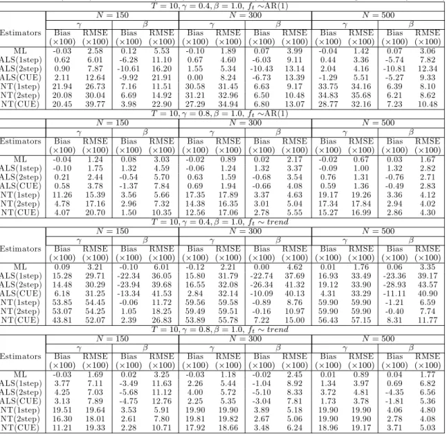
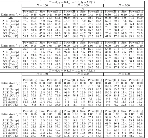
4.1.1 Results for the AR(1) case
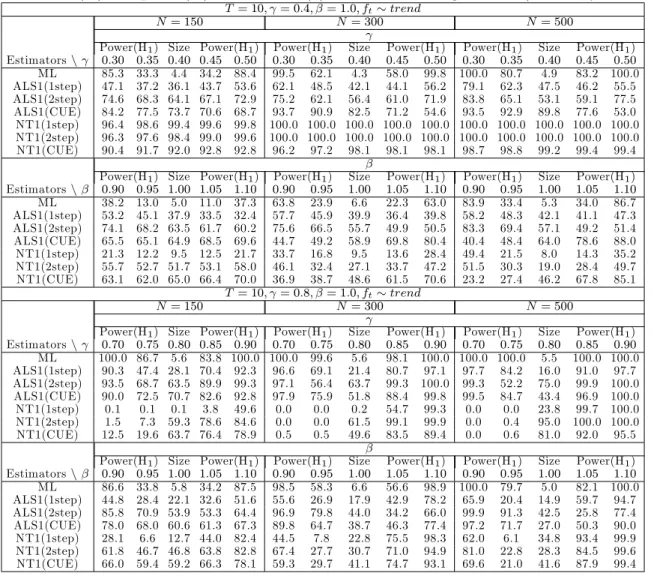
The simulation results for the AR(1) case are presented in Tables 1 to 4.6,7 In terms of bias and RMSE, the transformed ML estimator performs well for all cases. As the sample sizeN and/orT increases, the RMSE decreases irrespective of the value of the autoregressive parameter and the speci…cation used for ft:With regard to inference, the ML estimator performs well in that it has
correct size for all combinations ofN andT. Power performance is satisfactory though there is the tendency for the ML estimator to display low power for small positive departures from the null. For example, when = 0:8; T = 6 and N =f150;300g;the power is quite low for the alternative
= 0:9when testing the null = 0:8. This tendency is also evident whenftis generated as a time
trend. Contrary to the well behaved …nite sample properties of the transformed ML estimator, the performance of the GMM estimators are not generally good. In terms of bias and RMSE, the GMM estimators are substantially worse than the transformed ML estimator. With regard to size, the one-step ALS-GMM estimator displays empirical sizes close to the nominal level in many cases. However, its power is much lower as compared to that of the transformed ML estimator.
4.2 ARX(1) model with a single factor
The observations on yit for the ARX(1) model are generated as
yit = i+ yi;t 1+ xit+ it; fori= 1;2; :::; N;t= S+ 1; S+ 2; ::;0;1; :::; T; it = ift+uit,uit iidN(0; 2):
As in the AR(1) case, for values ofj j not too close to unity we setyi; S = 0 and note that forS
su¢ ciently large
yi0 t 1 1 i+ S 1 X j=0 jx i; j+ S 1 X j=0 j i; j:
The regressors,xit, are generated as
xit= i+#ift+xit; ; xit = xxi;t 1+ p
1 2
x"it; (35)
with xi; S = 0, fort= S+ 1; :::;0;1; :::; T, where j xj<1; i iidN(0;1),"it iidN(0;1) and
ftis generated as in the AR(1) case. We set x= 0:8which yields relatively persistence regressors.
We generate the factor loadings independently as
#i iidN(0:5; 2#); i iidN(0:5; 2); (36)
6
For the starting values in the optimization routine used to compute the ML estimators, we use ini = ( ini; !ini;q0
ini)0 with ini U[ 0:999;0:999],!ini U[1;2]andqt;ini U[ 1;1]where qt;iniis the tth element ofqini.
In addition ! needs to satisfy ! > (T 1)=T since j j = 1 +T(! 1) > 0: Speci…cally, we use …ve such sets of random starting values and choose the largest among the maximum of the log-likelihood values as the estimate of the ML estimator. Similarly, for the one-step ALS and NT GMM estimators we use …ve sets of starting values
ini;ALS= ( ini; 0ini)0 and ini;N T= ( ini;r0ini)0 respectively, where ini U[ 0:999;0:999], t;ini U[ 1;1]with t;inithetth element of ini;andrt;ini U[ 1;1]withrt;inithetth element ofrini:We select the smallest among
the minimum values of the objective function as the estimate of the one-step ALS and NT GMM estimators. For the two-step and continuous-updating ALS and NT GMM estimators we use the one-step estimates as the starting value of the optimization routine.
7In certain cases, the Hessian evaluated at the global maximum for the ML estimator was not positive de…nite.
The simulation draw for these cases was discarded and an additional draw was generated until the total number of simulations with a positive de…nite Hessian reached 1,000. The number of these additional draws decreased for a …xedT asN increased, and asT increased for allN.
and to ensure that the …xed e¤ects, i, are correlated with the regressors, as well as with the errors, we generate them as i =T 1 T X t=1 xit+ if+ui+vi;
where as in the AR(1) case,f =T 1PTt=1ft,ui =T 1PTt=1uit and vi iidN(0;1).
We set the remaining parameters bearing in mind that in the case of ARX(1) panels the average R2 is at least as large as 2. In particular, from the results for theR2 derived in Section A.5 of the Appendix we have that
R2y = 2V ar(x it) + h N 1PNi=1c2i T 1PTt=1ft2 + 2i 2 2V ar(x it) + N 1PNi=1c2i T 1 PT t=1ft2 + 2 2;
with the equality holding when = 0 and where ci = #i+ i. In view of (35)V ar(xit) = 1 and
without loss of generality we set = 1. Also, recall that T 1PTt=1ft2= 1. For comparability with the AR(1) case we set = (0:4;0:8) and determine 2; 2;and 2# such that R2y 2 = 0:1. To this end we note that
R2y 2 = 1
2
1 +N 1PN
i=1c2i + 2
= 0:1:
Further, for su¢ ciently large N and noting that i and #i are generated independently (see (36))
it follows that
N 1PNi=1c2i !p 2 2#+ 2 +
1
4(1 + )
2: Hence with = 1we have
R2y 2 = 1
2
2 + 2
#+ 2 + 2
= 0:1:
We set 2 = 2#= 2 and using the above result we obtain 2= 0:8 2
0:3 >0:
Finally, we consider the same combinations ofTandN as in the AR(1) case, namelyT =f6;10g
and N =f150;300;500g;and discard the …rst 50 observations basing estimation on the remaining observations over the period t = 0;1; ::::T. Note that after …rst-di¤erencing we end up with T observations for estimation of and . The standard errors used for inference are based on the same formulas as those used in the AR(1) case with all derivatives computed numerically.
We report simulation results for the same set of statistics as in the AR(1) case, for both and , including size and power. Power is computed for the null values of ( ; ) = f0:4;1:0g and
( ; ) = f0:8;1:0g. As previously, all tests are carried out at the 5% signi…cance level and all experiments are replicated 1,000 times.
Under strict exogeneity, for the ALS and NT GMM estimators there are so many moment conditions and using all of them causes a large …nite sample bias. Hence, we use only a subset of moment conditions for the exogenous variable xit: Speci…cally, for ALS GMM we use zit =
(yi0; :::; yi;t 1; xit; :::; xiT)0;since wit and W•it in (26) containxit and xi;T m; :::; xiT:Similarly, for
NT GMM we use zit = (yi0; :::; yi;t m 2; xi1; :::; xit)0: Recall that m is the number of unobserved
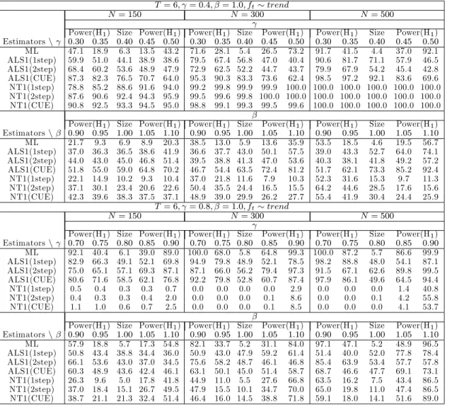
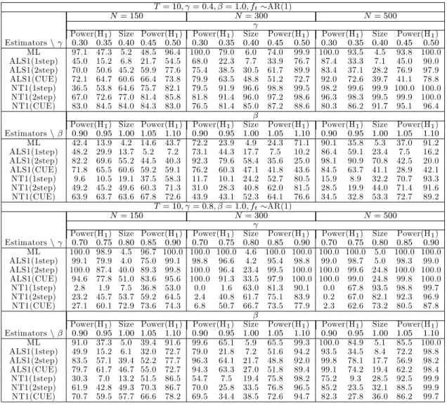
4.2.1 Results for the ARX(1) case
Simulation results for the ARX(1) model are summarized in Tables 5 to 8.8 In terms of bias and RMSE, the results are very similar to the AR(1) case. As the sample size increases, the RMSE decreases in all cases. The sizes are close to the nominal level in all cases and, contrary to the AR(1) case, the power is reasonably high even for = 0:8 and N = 150 irrespective of the speci…cation offt. The augmentation of the AR(1) model with exogenous regressors has also
bene…ted the GMM estimators who show improved performance as compared to the results obtained for the AR(1) model. However, the transformed ML estimator continues to outperform the GMM estimators (sometimes substantially) both in terms of bias and RMSE. In terms of size, all the GMM estimators exihibit large size distortions in almost all cases. An exception is the one-step NT-GMM with T = 6, = 0:8 and ft AR(1). In this case, the empirical size is close to the
nominal one, but power is lower than the transformed ML estimator.
4.3 AR(1) model with two factors
The observations on yit for the AR(1) model are generated as
yit = i+ yi;t 1+ it; fori= 1; :::; N; t= S+ 1; :::; 1;0;1; ::; T it = 1if1t+ 2if2t+uit= 0ift+uit; uit iidN(0; 2);
where ft= (f1t; f2t)0 and i = ( 1i; 2i)0, with the initial values of yit forj j <1 dealt with as in
the single factor case.
The unobserved common factors, f`t, are generated as
f`t = f `f`;t 1+ q
1 2f `"f `t,"f `t iidN(0;1), for`= 1;2;t= S+ 1; :::; 1;0;1; ::; T;
with f `= 0:9, and without loss of generalityf`; S = 0. As in the single factor case, we scale the
resultant f`t values such that T 1PTt=1f`t2 = 1 (the past values f`t fort = S+ 1; :::; 1;0 are
not scaled) to ensure a particular average value of …t.
The factor loadings, i = ( 1i; 2i)0 are generated independently of the error terms and all other
variables in‡uencing yit as
`i= + `i; with = 1and `i iidN(0;1).
The …xed e¤ects, i, are allowed to be correlated with the errors by generating them as i =T 1( i1+ i2+:::+ iT) +vi = 1if1+ 2if2+ui+vi;
wheref` =T 1PTt=1f`t,`= 1;2; ui =T 1PTt=1uit, and vi iidN(0;1).
As mentioned earlier, since the average …t of the panel AR(1) model is solely determined by (a result which holds irrespective of the number of factors) we set 2
u = 1.
8
As starting values, in the case of the ML estimation we use ini = ('0ini; !ini;q0ini)0 with 'ini = (bini; 0
ini; ini; ini)0;wherebiniand iniare obtained as the OLS estimates of (19), ini U[0;1];and the
remain-ing parameters are generated as in the AR(1) case usremain-ing …ve sets of startremain-ing values. For the one-step ALS and NT GMM estimators we use ini;ALS= ( ini; ini; 0ini)0and ini;N T= ( ini; ini;r0ini)0respectively, where ini U[0;1];
and the remaining parameters are generated as in the AR(1) case using …ve sets of starting values. For the CUE, for both ALS and NT we use the parameter estimates obtained from the one-step GMM.
4.3.1 Results for the AR(1) case
Simulation results for the AR(1) model are provided in Tables 9 and 10. Since the single factor results showed that the GMM estimators do not work well, we consider here the transformed ML estimator only. From the tables we …nd that the behaviour of the proposed estimator for the two factor case is similar to that of the single factor case. In particular, the bias of the transformed ML estimator is very small and RMSE decreases as N increases. In terms of inference, sizes are close to the nominal level and power is relatively high except for some cases with = 0:8:
4.4 ARX(1) model with two factors
The dependent variable, yit, for the ARX(1) model is generated as
yit = i+ yi;t 1+ xit+ it; fori= 1;2; :::; N;t= S+ 1; S+ 2; ::;0;1; :::; T); it = 0ift+uit,uit iidN(0; 2):
The regressors,xit, are generated as
xit= i+#0ift+xit; ; xit= xxi;t 1+ p
1 2
x"it; (37)
withxi; S = 0fort= S+ 1; :::;0;1; :::; T, where#i= (#1i; #2i)0, i iidN(0;1),"it iidN(0;1);
and f`t; ` = 1;2; are generated as in the AR(1) case, and x = 0:8. The factor loadings #i =
(#1i; #2i)0 and i= ( 1i; 2i)0 are generated independently as
#`i iidN(0:5; 2`#); `i iidN(0:5; 2` ); `= 1;2; (38)
and to ensure that the …xed e¤ects, i, are correlated with the regressors, as well as with the errors,
as in the single factor case we generate them as
i=xi+ 1if1+ 2if2+ui+vi;
wherexi=T 1PTt=1xit, and the remaining parameters are set as in the two factor AR(1) model.
In setting the remaining parameters, using results in Section A.5 of the Appendix, for the two factor case we have
Ry2= 2V ar(x it) + h N 1PNi=1c21i T 1PTt=1f12t + N 1PNi=1c22i T 1PTt=1f22t + 2 i 2 2V ar(x it) + N 1PNi=1c21i T 1PTt=1f12t + N 1PNi=1c22i T 1PTt=1f22t + 2 2;
where c`i = #`i+ `i, ` = 1;2. From (37) we have that V ar(xit) = 1 and we set = 1. For
comparability with the AR(1) case = (0:4;0:8) and 2; 2` ; and 2`#; ` = 1;2; are determined such thatR2y 2= 0:1;as in the single factor case. Thus, recalling that T 1PTt=1f`t2 = 1
R2y 2= 1 2 1 +N 1PN i=1c21i+N 1 PN i=1c22i+ 2 = 0:1;
and for su¢ ciently large N since i and #i are generated independently (see (38)) we have
N 1PNi=1c`i2 !p 2 2`#+ 2` +
1
4(1 + )
2; for`= 1;2: For = 1 we then obtain
R2y 2 = 1
2
3 + 21#+ 21 + 22#+ 22 + 2 = 0:1:
Setting 2
1#= 21 = 22#= 22 = 2 and using the above result yields 2= 0:7 2
4.4.1 Results for the ARX(1) case
Simulation results for the ARX(1) model are provided in Tables 11 and 12. As in the AR(1) case only the transformed ML estimator is considered. The results show that bias is very small and that RMSE decreases as N and T increase. In addition, size is close to its nominal value and power is high in all cases.
5
Conclusion
In this paper we proposed the transformed maximum likelihood estimator for short dynamic panel data models with interactive …xed e¤ects. This is a natural extension of Hsiao, Pesaran, and Tahmiscioglu (2002) to incorporate a factor structure in the error, while retaining the advantages of the transformed likelihood approach. Monte Carlo simulations were carried out to investigate the …nite sample behaviour of the proposed estimator and to compare its performance with several GMM estimators available in the literature. The simulation results showed that the ML estimator performs well in …nite samples and outperforms the GMM estimators in almost all cases considered. In our analysis we assumed that the number of factors is known. Estimating the number of factors in the current setting whereT is short and N tends to in…nity is a topic for future research.
Table 1: Bias( 100) and RMSE( 100) for the AR(1) model with a single factor (T = 6)
T = 6; = 0:4; ft AR(1)
N= 150 N= 300 N= 500
Estimator Bias RMSE Bias RMSE Bias RMSE ( 100) ( 100) ( 100) ( 100) ( 100) ( 100) ML 0.34 6.26 0.01 4.27 -0.16 3.31 ALS(1step) -17.20 33.97 -16.65 30.94 -17.82 29.22 ALS(2step) -15.94 32.21 -16.14 29.60 -16.62 27.89 ALS(CUE) -16.51 33.99 -14.99 29.36 -17.08 28.87 NT(1step) -58.44 60.78 -60.38 61.31 -61.05 61.62 NT(2step) -57.94 60.32 -60.58 61.38 -61.31 61.76 NT(CUE) -64.14 66.30 -65.22 65.72 -65.35 65.64 T = 6; = 0:8; ft AR(1) N= 150 N= 300 N= 500
Estimator Bias RMSE Bias RMSE Bias RMSE ( 100) ( 100) ( 100) ( 100) ( 100) ( 100) ML -0.14 7.35 0.04 5.63 0.15 4.71 ALS(1step) -34.26 48.24 -28.17 39.85 -27.57 37.15 ALS(2step) -35.26 49.17 -29.50 40.56 -28.70 37.97 ALS(CUE) -33.98 50.34 -27.33 40.68 -26.74 37.55 NT(1step) -59.14 85.47 -65.45 89.77 -71.95 93.70 NT(2step) -56.65 82.48 -60.66 84.75 -66.43 87.70 NT(CUE) -57.22 83.70 -58.49 81.90 -61.448 83.58 T = 6; = 0:4; ft trend N= 150 N= 300 N= 500
Estimator Bias RMSE Bias RMSE Bias RMSE ( 100) ( 100) ( 100) ( 100) ( 100) ( 100) ML 0.23 8.12 -0.02 5.45 0.05 4.16 ALS(1step) -19.00 33.04 -19.87 27.96 -19.84 24.86 ALS(2step) -18.62 32.37 -19.63 27.68 -19.11 23.95 ALS(CUE) -18.83 34.47 -19.58 28.67 -18.95 24.38 NT(1step) -12.74 54.24 -20.47 58.26 -28.74 60.59 NT(2step) -13.36 55.40 -21.22 59.06 -29.30 61.14 NT(CUE) -18.64 62.90 -24.75 62.83 -31.45 63.35 T = 6; = 0:8; ft trend N= 150 N= 300 N= 500
Estimator Bias RMSE Bias RMSE Bias RMSE ( 100) ( 100) ( 100) ( 100) ( 100) ( 100) ML -3.21 13.36 -1.68 10.36 -0.43 8.34 ALS(1step) -34.76 51.98 -34.05 52.22 -35.43 53.05 ALS(2step) -37.44 54.36 -36.70 55.01 -36.99 54.37 ALS(CUE) -35.42 56.23 -34.47 55.11 -35.13 54.39 NT(1step) -49.95 63.27 -61.37 73.58 -71.26 81.07 NT(2step) -50.83 64.44 -61.79 74.83 -72.50 82.81 NT(CUE) -60.29 80.38 -72.93 89.58 -83.87 96.77
Notes:yitis generated asyit= i+ yi;t 1+ it; it= ift+uit; uit iidN(0; 2); i= 1;2; :::; N;t= 49;48; :::0;1; :::; T;with yi; 50= 0and 2= 1. The factor is generated as: ft= fft 1+
q
1 2f"f t,"f t iidN(0;1), fort= 49;48; :::0;1; :::; T;
withf 50= 0;and f = 0:9;in the case whereft AR(1);ft= 0for allt= 49;48; :::0;andft=tfor1;2; :::; T;in the case
whereft trend:Under both speci…cations offt, the resultantftvalues are scaled such thatT 1PT
t=1ft2= 1. The values of ftfort= 49;48; :::0are not scaled. The factor loadings, i, are generated as i= + i with = 1and i iidN(0;1). The
…xed e¤ects, i, are generated as i=T 1( i1+ i2+:::+ iT)+vi= if+ui+vi;wheref=T 1
PT
t=1ft,ui=T 1
PT t=1uit, andvi iidN(0;1). Eachftis generated once and the samef0
tsare used throughout the replications. The …rst 50 observations
are discarded. ML is the proposed transformed maximum likelihood estimator. ALS(j) and NT(j) withj= 1step;2step; CU E
are the one step, two step and continuous updating GMM estimators of Ahn et al. (2013), and Nauges and Thomas (2003), respectively. All experiments are based on 1,000 replications.
Table 2: Bias( 100) and RMSE( 100) (T = 10) for the AR(1) model with a single factor
T = 10; = 0:4; ft AR(1)
N= 150 N= 300 N= 500
Estimator Bias RMSE Bias RMSE Bias RMSE ( 100) ( 100) ( 100) ( 100) ( 100) ( 100) ML 0.30 4.47 0.01 3.11 -0.09 2.28 ALS(1step) 15.18 23.26 10.06 18.99 6.69 15.39 ALS(2step) 12.45 20.40 7.03 15.88 3.58 11.42 ALS(CUE) 11.66 19.92 3.68 13.94 0.91 9.66 NT(1step) -35.40 41.02 -43.60 44.20 -47.11 47.48 NT(2step) -41.82 47.14 -51.89 52.29 -55.49 55.69 NT(CUE) -56.39 61.07 -61.56 61.62 -61.87 61.90 T = 10; = 0:8; ft AR(1) N= 150 N= 300 N= 500
Estimator Bias RMSE Bias RMSE Bias RMSE ( 100) ( 100) ( 100) ( 100) ( 100) ( 100) ML 0.30 6.01 0.12 4.59 0.06 3.63 ALS(1step) -5.35 9.68 -5.01 9.08 -4.51 9.84 ALS(2step) -8.12 11.72 -7.58 11.15 -6.71 11.49 ALS(CUE) -3.92 10.87 -3.49 9.64 -3.04 10.27 NT(1step) 2.32 31.97 0.98 36.27 -0.05 40.53 NT(2step) -5.33 34.26 -5.70 37.08 -5.72 40.21 NT(CUE) -7.64 37.24 -9.28 39.41 -10.04 39.70 T = 10; = 0:4; ft trend N= 150 N= 300 N= 500
Estimator Bias RMSE Bias RMSE Bias RMSE ( 100) ( 100) ( 100) ( 100) ( 100) ( 100) ML 0.21 4.18 0.21 4.18 -0.09 2.28 ALS(1step) -9.06 12.94 -9.06 12.94 6.69 15.39 ALS(2step) -9.59 13.61 -9.59 13.61 3.58 11.42 ALS(CUE) -11.77 15.28 -11.77 15.28 0.91 9.66 NT(1step) -24.10 52.37 -24.10 52.37 -47.11 47.48 NT(2step) -27.60 55.35 -27.60 55.35 -55.49 55.69 NT(CUE) -24.64 61.13 -24.64 61.13 -61.87 61.90 T = 6; = 0:8; ft trend N= 150 N= 300 N= 500
Estimator Bias RMSE Bias RMSE Bias RMSE ( 100) ( 100) ( 100) ( 100) ( 100) ( 100) ML -0.10 6.92 0.15 5.39 -0.06 4.24 ALS(1step) -10.74 18.61 -11.93 21.10 -13.84 23.54 ALS(2step) -11.89 16.89 -12.85 19.63 -17.46 24.11 ALS(CUE) -10.15 20.96 -12.66 24.69 -16.94 28.01 NT(1step) -46.57 60.17 -60.55 72.32 -75.19 83.16 NT(2step) -49.44 63.01 -63.07 75.26 -78.42 87.33 NT(CUE) -56.11 77.72 -77.00 93.18 -95.74 105.41 See notes to Table 1.
Table 3: Size(%) and power(%) for the AR(1) model with a single factor (T = 6)
T = 6; = 0:4; ft AR(1)
N= 150 N= 300 N= 500
Power(H1) Size Power(H1) Power(H1) Size Power(H1) Power(H1) Size Power(H1) Estimatorsn 0:30 0:35 0:40 0:45 0:50 0:30 0:35 0:40 0:45 0:50 0:30 0:35 0:40 0:45 0:50 ML 38.1 14.5 5.4 12.1 40.0 64.2 23.2 4.7 20.8 65.5 83.8 35.1 4.8 28.6 85.6 ALS(1step) 6.1 4.8 3.7 3.8 4.3 8.5 5.9 4.8 4.2 4.5 13.0 7.0 4.1 3.1 3.2 ALS(2step) 15.9 13.7 11.6 11.1 10.9 26.0 18.8 14.0 11.9 11.6 33.6 23.2 15.9 12.6 11.9 ALS(CUE) 13.4 11.2 10.1 9.0 8.6 17.0 11.0 8.3 6.6 6.1 25.0 17.1 11.4 8.1 7.7 NT(1step) 92.3 89.4 86.0 82.1 77.0 99.9 99.8 99.1 97.8 96.0 100.0 100.0 100.0 99.9 99.6 NT(2step) 95.6 94.0 91.7 89.1 83.6 100.0 99.7 99.3 98.9 98.5 100.0 100.0 100.0 100.0 99.8 NT(CUE) 99.0 99.0 98.8 97.8 95.4 100.0 100.0 100.0 100.0 100.0 100.0 100.0 100.0 100.0 100.0 T = 6; = 0:8; ft AR(1) N= 150 N= 300 N= 500
Power(H1) Size Power(H1) Power(H1) Size Power(H1) Power(H1) Size Power(H1) Estimatorsn 0:70 0:75 0:80 0:85 0:90 0:70 0:75 0:80 0:85 0:90 0:70 0:75 0:80 0:85 0:90 ML 30.9 15.6 5.8 2.3 5.6 42.2 20.7 6.4 1.7 12.0 55.4 25.8 4.8 2.6 47.3 ALS(1step) 8.1 6.4 5.3 4.4 3.7 8.8 7.1 5.6 4.6 3.5 8.8 7.7 6.2 4.6 3.6 ALS(2step) 19.1 16.1 13.9 11.8 10.0 18.6 15.7 12.7 10.9 8.3 18.4 15.8 12.8 10.5 8.7 ALS(CUE) 15.1 12.8 10.9 9.4 7.8 15.9 13.6 11.8 9.7 7.8 15.6 13.8 11.5 10.0 8.0 NT(1step) 56.1 55.6 55.2 54.5 54.0 63.4 63.3 62.9 62.7 62.7 69.2 69.0 68.9 68.9 69.7 NT(2step) 59.1 58.6 58.5 58.1 57.6 64.3 63.9 63.9 63.8 64.2 69.4 69.3 69.3 69.3 70.5 NT(CUE) 54.1 53.8 53.5 53.3 53.4 57.8 57.7 57.7 57.5 57.7 57.6 57.6 57.6 57.7 59.1 T = 6; = 0:4; ft trend N= 150 N= 300 N= 500
Power(H1) Size Power(H1) Power(H1) Size Power(H1) Power(H1) Size Power(H1) Estimatorsn 0:30 0:35 0:40 0:45 0:50 0:30 0:35 0:40 0:45 0:50 0:30 0:35 0:40 0:45 0:50 ML 28.7 14.4 6.0 9.6 23.9 45.4 18.9 5.0 13.7 43.6 66.3 24.0 5.8 21.0 67.6 ALS(1step) 6.4 5.4 4.1 3.3 2.6 9.4 6.5 3.8 2.0 1.2 18.5 13.2 8.0 4.5 2.2 ALS(2step) 14.1 10.8 9.9 8.2 6.8 19.7 15.2 10.5 7.6 5.3 27.1 19.3 13.0 8.3 5.0 ALS(CUE) 9.8 8.2 7.3 5.6 4.1 15.0 10.6 7.2 4.7 3.1 22.0 15.2 10.0 5.9 3.1 NT(1step) 47.0 45.5 43.1 40.6 38.2 67.2 67.5 68.7 71.8 74.0 78.3 84.1 90.2 93.7 95.7 NT(2step) 48.8 47.7 47.5 47.4 46.9 67.7 69.3 71.5 75.5 78.8 79.5 85.8 91.0 94.5 96.5 NT(CUE) 56.6 55.7 56.3 56.7 58.6 69.6 71.4 74.5 78.7 81.8 79.3 85.5 91.5 94.8 96.6 T = 6; = 0:8; ft trend N= 150 N= 300 N= 500
Power(H1) Size Power(H1) Power(H1) Size Power(H1) Power(H1) Size Power(H1) Estimatorsn 0:70 0:75 0:80 0:85 0:90 0:70 0:75 0:80 0:85 0:90 0:70 0:75 0:80 0:85 0:90 ML 22.5 16.0 10.3 5.3 2.3 21.9 15.1 7.9 3.1 1.3 25.2 13.4 5.1 1.7 1.4 ALS(1step) 4.1 3.2 2.8 1.8 1.1 6.0 4.5 3.0 2.3 1.8 7.3 5.0 3.7 2.8 2.0 ALS(2step) 13.5 11.5 8.1 6.8 5.0 15.5 13.3 11.5 9.7 7.2 20.4 16.5 14.2 10.7 8.3 ALS(CUE) 10.0 7.7 5.9 4.6 3.9 13.3 11.3 9.3 7.6 6.1 15.1 12.2 9.5 7.4 6.6 NT(1step) 32.2 31.7 30.8 30.1 28.2 46.6 45.8 44.6 43.7 42.9 60.2 59.6 59.1 57.8 56.9 NT(2step) 31.8 31.0 30.8 30.4 29.4 46.4 45.6 44.9 44.0 42.9 59.5 59.0 58.5 57.8 56.6 NT(CUE) 41.4 41.0 41.0 40.4 40.0 52.8 52.7 52.4 52.0 51.6 64.6 64.4 64.3 64.0 63.6 See notes to Table 1.
Table 4: Size(%) and power(%) for the AR(1) model with a single factor (T = 10)
T = 10; = 0:4; ft AR(1)
N= 150 N= 300 N= 500
Power(H1) Size Power(H1) Power(H1) Size Power(H1) Power(H1) Size Power(H1) Estimatorsn 0:30 0:35 0:40 0:45 0:50 0:30 0:35 0:40 0:45 0:50 0:30 0:35 0:40 0:45 0:50 ML 62.5 20.2 6.3 21.6 66.9 89.2 37.9 5.7 38.0 91.1 99.1 58.4 3.2 54.8 99.7 ALS(1step) 13.6 16.3 20.0 22.4 25.3 12.1 15.3 20.9 25.8 29.8 11.6 14.2 19.0 23.7 29.3 ALS(2step) 55.8 60.4 66.9 70.6 75.5 51.3 47.2 50.7 58.4 68.2 58.5 39.9 34.9 45.2 63.9 ALS(CUE) 24.9 25.9 29.7 31.7 33.0 36.2 29.2 24.0 25.0 30.0 48.2 30.1 18.7 20.7 36.5 NT(1step) 94.3 91.0 86.8 78.4 68.3 99.9 99.7 98.8 97.7 93.4 100.0 100.0 100.0 99.9 99.8 NT(2step) 99.1 98.9 98.3 96.7 94.6 100.0 100.0 100.0 100.0 99.9 100.0 100.0 100.0 100.0 100.0 NT(CUE) 98.4 98.4 98.3 98.4 98.4 100.0 100.0 100.0 100.0 100.0 100.0 100.0 100.0 100.0 100.0 T = 10; = 0:8; ft AR(1) N= 150 N= 300 N= 500
Power(H1) Size Power(H1) Power(H1) Size Power(H1) Power(H1) Size Power(H1) Estimatorsn 0:70 0:75 0:80 0:85 0:90 0:70 0:75 0:80 0:85 0:90 0:70 0:75 0:80 0:85 0:90 ML 37.0 18.1 4.7 3.9 15.8 53.8 24.9 4.8 5.0 54.5 72.1 33.8 5.0 13.4 84.5 ALS(1step) 25.6 16.5 4.6 1.1 4.1 26.2 16.6 7.3 2.5 4.9 29.1 17.0 7.5 4.6 9.0 ALS(2step) 79.5 74.2 61.3 45.0 35.5 77.2 70.9 59.1 43.8 35.8 72.7 66.7 58.3 45.1 37.0 ALS(CUE) 29.0 23.3 18.0 15.0 17.6 37.7 28.8 21.9 15.7 20.7 38.1 30.3 23.9 16.8 21.3 NT(1step) 10.3 9.9 8.6 7.8 7.4 11.8 11.4 11.3 11.0 10.8 13.2 13.1 13.1 13.1 13.9 NT(2step) 21.1 18.9 17.2 18.1 21.1 18.0 16.6 15.6 15.2 19.5 18.2 17.4 16.1 16.4 22.9 NT(CUE) 25.8 23.2 21.3 21.9 27.4 23.7 21.7 20.9 21.3 26.9 19.8 18.1 17.6 19.4 25.0 T = 10; = 0:4; ft trend N= 150 N= 300 N= 500
Power(H1) Size Power(H1) Power(H1) Size Power(H1) Power(H1) Size Power(H1) Estimatorsn 0:30 0:35 0:40 0:45 0:50 0:30 0:35 0:40 0:45 0:50 0:30 0:35 0:40 0:45 0:50 ML 66.7 23.1 5.5 23.6 71.2 92.6 40.6 4.8 42.6 93.9 99.1 63.3 4.7 58.7 99.9 ALS(1step) 23.3 13.7 6.7 2.6 2.5 41.3 32.0 16.6 5.7 0.9 48.2 44.4 30.9 11.8 1.7 ALS(2step) 49.2 35.4 20.2 11.6 10.2 69.4 59.0 36.5 15.7 6.6 79.6 75.3 53.1 21.0 4.9 ALS(CUE) 30.2 22.8 14.9 9.0 6.5 45.3 38.9 26.6 11.9 4.7 54.1 51.5 38.5 16.4 4.7 NT(1step) 89.3 90.4 90.4 89.2 86.1 99.9 99.8 99.8 99.6 99.5 100.0 100.0 100.0 100.0 100.0 NT(2step) 97.6 97.8 97.6 97.1 96.1 100.0 100.0 100.0 100.0 100.0 100.0 100.0 100.0 100.0 100.0 NT(CUE) 80.2 80.6 80.6 80.7 80.7 97.3 97.3 97.3 97.3 97.3 99.8 99.8 99.8 99.8 99.8 T = 10; = 0:8; ft trend N= 150 N= 300 N= 500
Power(H1) Size Power(H1) Power(H1) Size Power(H1) Power(H1) Size Power(H1) Estimatorsn 0:70 0:75 0:80 0:85 0:90 0:70 0:75 0:80 0:85 0:90 0:70 0:75 0:80 0:85 0:90 ML 31.0 15.5 4.5 2.1 11.3 44.0 19.9 5.4 6.6 39.4 64.1 26.5 4.8 14.5 61.4 ALS(1step) 6.5 2.8 1.0 0.3 0.8 10.5 4.5 1.8 1.2 2.0 9.4 5.2 2.3 2.0 3.3 ALS(2step) 41.9 35.4 25.6 18.1 13.8 39.0 31.2 23.1 16.2 15.0 42.6 38.8 31.9 23.0 18.0 ALS(CUE) 19.4 16.1 14.2 13.2 11.9 25.6 22.2 19.3 16.6 16.8 32.8 29.7 26.7 24.6 23.2 NT(1step) 47.0 46.0 44.8 43.3 41.8 67.8 67.3 66.5 65.7 64.2 82.4 81.9 81.2 80.6 80.2 NT(2step) 46.7 45.3 44.6 43.5 43.0 63.6 62.8 62.3 61.5 60.4 79.3 79.1 78.6 77.9 77.4 NT(CUE) 47.9 47.4 47.3 47.0 46.9 66.8 66.7 66.5 66.2 66.2 82.2 82.1 82.1 82.1 82.1 See notes to Table 1.
Table 5: Bias( 100) and RMSE( 100) for the ARX(1) model with a single factor (T = 6)
T= 6; = 0:4; = 1:0; ft AR(1)
N= 150 N= 300 N= 500
Estimators Bias RMSE Bias RMSE Bias RMSE Bias RMSE Bias RMSE Bias RMSE ( 100) ( 100) ( 100) ( 100) ( 100) ( 100) ( 100) ( 100) ( 100) ( 100) ( 100) ( 100) ML -0.19 4.29 -0.05 7.41 0.03 3.01 0.05 5.26 -0.05 2.30 0.01 4.08 ALS(1step) 0.81 16.60 -3.11 17.23 -0.87 11.56 -1.59 11.85 -1.71 8.16 -0.86 8.51 ALS(2step) 2.10 17.47 -5.20 19.40 1.69 11.82 -4.80 13.42 1.76 8.32 -4.47 9.97 ALS(CUE) 2.46 22.58 -7.08 23.84 -0.70 15.87 -4.44 15.66 -2.51 11.59 -2.93 11.07 NT(1step) -3.70 32.16 4.70 14.58 8.52 24.51 7.37 12.02 15.80 20.97 8.52 10.84 NT(2step) -6.23 35.96 4.09 16.28 6.58 27.22 6.96 12.90 14.76 21.98 8.07 11.01 NT(CUE) 17.04 41.42 0.60 22.77 26.21 35.06 4.72 13.98 29.58 31.63 5.70 10.90 T= 6; = 0:8; = 1:0; ft AR(1) N= 150 N= 300 N= 500
Estimators Bias RMSE Bias RMSE Bias RMSE Bias RMSE Bias RMSE Bias RMSE ( 100) ( 100) ( 100) ( 100) ( 100) ( 100) ( 100) ( 100) ( 100) ( 100) ( 100) ( 100) ML -0.06 2.38 -0.07 4.33 -0.10 1.74 0.09 3.14 -0.01 1.32 0.01 2.42 ALS(1step) -1.35 5.39 3.03 8.29 -2.11 4.17 4.02 6.85 -2.32 3.16 4.29 5.56 ALS(2step) -0.33 5.20 1.52 7.97 -0.65 3.55 2.02 5.78 -0.67 2.28 2.23 4.26 ALS(CUE) -0.44 5.90 0.81 8.44 -1.15 3.93 1.87 5.76 -1.21 2.66 1.99 4.32 NT(1step) -1.37 14.76 0.51 6.36 5.89 12.26 0.83 4.57 9.39 11.85 0.79 3.65 NT(2step) -2.45 17.17 0.38 7.20 5.32 13.55 0.69 5.06 9.06 12.37 0.60 3.97 NT(CUE) 8.50 18.47 -0.09 8.50 14.21 16.97 0.14 5.51 16.50 17.16 0.01 4.22 T = 6; = 0:4; = 1:0; ft trend N= 150 N= 300 N= 500
Estimators Bias RMSE Bias RMSE Bias RMSE Bias RMSE Bias RMSE Bias RMSE ( 100) ( 100) ( 100) ( 100) ( 100) ( 100) ( 100) ( 100) ( 100) ( 100) ( 100) ( 100) ML -0.07 5.82 -0.28 8.96 0.07 3.98 -0.08 6.27 -0.07 2.95 0.01 4.77 ALS(1step) 9.07 36.37 -13.00 40.27 5.61 36.84 -8.65 40.08 3.71 37.09 -6.38 39.69 ALS(2step) 10.86 36.14 -16.42 41.33 10.57 34.73 -15.78 39.41 10.68 34.05 -15.65 38.38 ALS(CUE) 1.58 43.38 -7.24 48.41 -0.94 39.84 -2.94 42.45 -2.13 39.03 -1.24 40.83 NT(1step) 54.52 55.27 -4.96 16.36 59.27 59.32 -5.65 12.47 59.81 59.82 -6.11 10.67 NT(2step) 55.16 56.00 -6.97 20.08 59.47 59.52 -8.04 15.34 59.87 59.87 -8.68 13.38 NT(CUE) 55.52 57.40 -7.78 27.23 59.31 59.43 -7.13 18.07 59.82 59.83 -6.68 14.17 T = 6; = 0:8; = 1:0; ft trend N= 150 N= 300 N= 500
Estimators Bias RMSE Bias RMSE Bias RMSE Bias RMSE Bias RMSE Bias RMSE ( 100) ( 100) ( 100) ( 100) ( 100) ( 100) ( 100) ( 100) ( 100) ( 100) ( 100) ( 100) ML -0.09 3.10 -0.14 4.88 -0.11 2.18 0.04 3.44 -0.01 1.65 0.01 2.64 ALS(1step) 4.65 10.21 -4.82 14.47 4.23 9.69 -3.85 13.19 3.66 9.12 -2.99 12.24 ALS(2step) 6.54 10.13 -6.98 13.73 6.95 9.82 -7.09 12.28 7.41 9.79 -7.20 11.61 ALS(CUE) 4.71 10.38 -5.36 14.56 4.38 9.43 -4.24 11.94 4.06 8.87 -3.51 10.83 NT(1step) 18.93 19.50 1.40 6.85 19.86 19.87 1.49 4.93 19.90 19.90 1.44 3.99 NT(2step) 17.83 18.92 1.24 7.84 19.77 19.80 1.58 5.42 19.89 19.89 1.52 4.26 NT(CUE) 17.64 19.22 1.67 9.08 19.66 19.71 2.08 6.04 19.84 19.85 2.12 4.70 Notes: yit is generated as yit = i+ yi;t 1+ xit+ it; it = ift+uit; uit iidN(0; 2); i = 1;2; :::; N;t =
49;48; :::0;1; :::; T;with yi; 50 = 0 and xit = i+#ift+xit; ; xit = xxi;t 1 +
p
1 2
x"it; with xi; 50 = 0, fort = 49;48; :::0;1; :::; T, where x= 0:8; i iidN(0;1), and"it iidN(0;1):The factorftis generated as in the AR(1) case (see
notes to Table 1). The factor loadings,#i and i, are generated as#i iidN(0:5; #2)and i iidN(0:5; 2);respectively.
The …xed e¤ects, i, are generated as i=T 1PTt=1xit+ if+ui+vi;wheref=T 1
PT
t=1ft,ui=T 1
PT
t=1uit, and vi iidN(0;1). The remaining parameters are set at = 1; 2= 2
#= 2, with 2= (0:8 2)=0:3:Eachftis generated once
and the samef0
tsare used throughout the replications. The …rst 50 observations are discarded. ML is the proposed maximum
likelihood estimator. ALS(j) and NT(j) withj= 1step;2step; CU Eare the one step, two step and continuous updating GMM estimators of Ahn et al. (2013), and Nauges and Thomas (2003), respectively. All experiments are based on 1,000 replications.
Table 6: Bias( 100) and RMSE( 100) for the ARX(1) model with a single factor (T = 10)
T= 10; = 0:4; = 1:0; ft AR(1)
N= 150 N= 300 N= 500
Estimators Bias RMSE Bias RMSE Bias RMSE Bias RMSE Bias RMSE Bias RMSE ( 100) ( 100) ( 100) ( 100) ( 100) ( 100) ( 100) ( 100) ( 100) ( 100) ( 100) ( 100) ML -0.03 2.58 0.12 5.53 -0.10 1.89 0.07 3.99 -0.04 1.42 0.07 3.06 ALS(1step) 0.62 6.01 -6.28 11.10 0.67 4.60 -6.03 9.11 0.44 3.36 -5.74 7.82 ALS(2step) 0.90 7.87 -10.61 16.20 1.55 5.34 -10.43 13.14 2.04 4.16 -10.81 12.34 ALS(CUE) 2.11 12.64 -9.92 21.91 0.00 8.24 -6.73 13.39 -1.29 5.51 -5.27 9.33 NT(1step) 21.94 26.73 7.16 11.51 30.58 31.45 6.63 9.17 33.75 34.16 6.39 8.10 NT(2step) 20.08 30.04 6.69 14.92 31.21 32.96 6.50 10.48 34.83 35.68 6.21 8.62 NT(CUE) 20.45 39.77 3.98 22.90 27.29 34.94 6.80 13.07 28.77 32.16 7.23 10.48 T= 10; = 0:8; = 1:0; ft AR(1) N= 150 N= 300 N= 500
Estimators Bias RMSE Bias RMSE Bias RMSE Bias RMSE Bias RMSE Bias RMSE ( 100) ( 100) ( 100) ( 100) ( 100) ( 100) ( 100) ( 100) ( 100) ( 100) ( 100) ( 100) ML -0.04 1.24 0.08 3.03 -0.02 0.89 0.02 2.17 -0.02 0.67 0.03 1.67 ALS(1step) -0.10 1.75 1.32 4.59 -0.06 1.24 1.32 3.37 -0.09 1.00 1.32 2.82 ALS(2step) 0.21 2.44 -0.54 5.70 0.63 1.59 -0.68 3.54 0.76 1.31 -0.76 2.71 ALS(CUE) 0.58 3.78 -1.37 7.84 0.69 1.94 -0.66 4.08 0.59 1.36 -0.49 2.83 NT(1step) 11.26 15.39 3.56 5.66 17.35 17.89 3.37 4.63 19.17 19.26 3.36 4.12 NT(2step) 4.78 17.16 2.96 7.32 14.38 16.35 3.01 5.04 17.34 17.84 2.94 4.02 NT(CUE) 4.07 20.70 1.50 10.35 12.56 17.06 2.78 5.55 15.27 16.99 2.86 4.30 T = 10; = 0:4; = 1:0; ft trend N= 150 N= 300 N= 500
Estimators Bias RMSE Bias RMSE Bias RMSE Bias RMSE Bias RMSE Bias RMSE ( 100) ( 100) ( 100) ( 100) ( 100) ( 100) ( 100) ( 100) ( 100) ( 100) ( 100) ( 100) ML 0.09 3.21 -0.10 6.01 -0.12 2.21 0.00 4.62 0.01 1.76 0.06 3.35 ALS(1step) 15.28 29.71 -22.34 36.05 15.80 31.79 -22.74 37.69 16.93 33.49 -23.36 39.17 ALS(2step) 14.48 30.29 -23.94 39.68 16.55 32.08 -26.34 41.32 19.12 33.90 -28.93 43.57 ALS(CUE) 6.18 31.25 -13.34 41.53 2.84 32.14 -10.09 40.13 4.31 33.29 -11.11 40.90 NT(1step) 53.85 54.45 -0.06 11.72 59.56 59.58 -0.89 8.76 59.90 59.90 -1.21 6.59 NT(2step) 53.07 54.25 1.05 18.25 59.49 59.51 -0.16 10.97 59.90 59.90 -0.40 7.74 NT(CUE) 43.81 52.07 2.39 26.83 53.89 55.78 7.22 15.00 56.43 57.15 8.31 11.77 T = 10; = 0:8; = 1:0; ft trend N= 150 N= 300 N= 500
Estimators Bias RMSE Bias RMSE Bias RMSE Bias RMSE Bias RMSE Bias RMSE ( 100) ( 100) ( 100) ( 100) ( 100) ( 100) ( 100) ( 100) ( 100) ( 100) ( 100) ( 100) ML -0.03 1.69 0.02 3.25 -0.03 1.18 -0.02 2.45 0.01 0.89 0.04 1.77 ALS(1step) 3.77 7.11 -3.49 11.63 2.26 5.44 -1.04 8.92 1.34 3.97 0.69 6.82 ALS(2step) 4.25 7.03 -5.68 11.12 4.00 5.72 -5.10 8.33 3.72 4.81 -4.35 6.56 ALS(CUE) 3.13 7.89 -4.75 12.76 2.25 5.35 -3.04 7.81 1.73 3.78 -1.81 5.36 NT(1step) 19.51 19.64 3.53 5.91 19.90 19.90 3.89 5.18 19.90 19.90 4.06 4.80 NT(2step) 16.30 18.01 2.61 7.80 19.81 19.82 2.67 5.06 19.90 19.90 2.78 4.08 NT(CUE) 11.21 19.33 2.28 10.71 17.92 18.66 3.48 6.24 18.96 19.17 3.71 5.03 See notes to Table 5.
Table 7a: Size(%) and power(%) for the ARX(1) model with a single factor (T = 6; ft AR(1)) T = 6; = 0:4; = 1:0; ft AR(1)
N= 150 N= 300 N= 500
Power(H1) Size Power(H1) Power(H1) Size Power(H1) Power(H1) Size Power(H1) Estimatorsn 0:30 0:35 0:40 0:45 0:50 0:30 0:35 0:40 0:45 0:50 0:30 0:35 0:40 0:45 0:50 ML 68.2 25.0 5.8 21.6 65.6 91.9 38.9 7.1 42.5 92.2 99.0 60.6 5.9 61.4 99.0 ALS1(1step) 37.2 22.1 15.2 16.7 26.3 48.7 27.1 15.2 15.8 29.8 62.4 32.6 15.6 15.0 37.2 ALS1(2step) 45.3 32.8 25.6 28.8 38.9 44.1 28.2 19.7 27.9 48.6 47.9 25.7 18.0 35.1 63.2 ALS1(CUE) 56.3 48.2 41.7 40.0 46.0 62.0 47.1 37.7 36.1 39.5 70.1 50.7 35.1 30.5 39.8 NT1(1step) 29.5 31.6 35.2 38.1 41.4 19.8 26.8 35.6 45.5 57.5 16.7 30.4 46.1 61.3 73.0 NT1(2step) 41.6 43.4 45.8 49.4 54.9 33.8 40.0 48.7 53.6 61.8 25.4 38.2 51.3 62.3 72.5 NT1(CUE) 54.7 59.8 65.0 71.6 75.7 57.1 66.6 74.8 82.5 88.7 61.9 77.6 88.0 93.2 96.9 Power(H1) Size Power(H1) Power(H1) Size Power(H1) Power(H1) Size Power(H1) Estimatorsn 0:90 0:95 1:00 1:05 1:10 0:90 0:95 1:00 1:05 1:10 0:90 0:95 1:00 1:05 1:10 ML 26.3 10.6 3.9 9.7 23.3 47.6 14.7 4.2 15.9 46.3 68.0 21.2 4.7 22.0 68.4 ALS1(1step) 21.7 15.4 11.5 12.7 17.5 27.3 14.4 8.5 12.1 22.7 34.8 14.3 7.5 12.5 30.2 ALS1(2step) 34.0 24.5 20.4 21.8 27.3 44.1 26.9 15.8 14.1 21.9 60.5 32.8 16.7 11.8 23.0 ALS1(CUE) 41.1 32.4 29.5 30.2 34.4 43.3 29.4 20.7 21.5 29.9 50.7 28.8 17.1 16.5 31.0 NT1(1step) 13.3 12.8 14.4 21.0 34.2 10.1 11.0 22.1 39.7 61.2 6.6 10.4 32.1 60.1 84.6 NT1(2step) 23.7 21.5 24.2 32.1 44.5 17.5 17.1 26.8 44.5 62.0 11.4 14.2 35.0 61.3 81.9 NT1(CUE) 32.9 30.4 34.1 39.4 46.6 24.3 21.5 27.1 38.5 53.4 20.8 17.4 30.6 47.4 70.1 T = 6; = 0:8; = 1:0; ft AR(1) N= 150 N= 300 N= 500
Power(H1) Size Power(H1) Power(H1) Size Power(H1) Power(H1) Size Power(H1) Estimatorsn 0:70 0:75 0:80 0:85 0:90 0:70 0:75 0:80 0:85 0:90 0:70 0:75 0:80 0:85 0:90 ML 99.8 56.1 5.1 56.8 97.2 100.0 86.2 6.1 81.6 100.0 100.0 97.3 6.4 95.7 100.0 ALS1(1step) 92.9 55.9 14.6 18.7 62.6 99.3 81.5 16.5 23.4 80.7 99.9 95.7 21.2 27.8 94.4 ALS1(2step) 91.2 55.8 19.8 36.2 77.4 98.8 71.7 13.9 43.6 94.0 100.0 83.8 11.4 62.8 99.8 ALS1(CUE) 90.9 59.8 24.7 37.0 74.9 98.6 76.4 19.1 39.4 90.4 99.9 88.4 16.6 52.3 98.5 NT1(1step) 9.2 6.6 5.0 4.0 6.3 2.7 1.6 1.6 7.1 16.7 0.3 0.3 6.2 17.3 30.9 NT1(2step) 14.3 11.8 10.4 10.9 15.1 5.4 4.3 4.5 15.6 27.2 0.9 0.7 11.5 24.1 36.2 NT1(CUE) 8.7 8.2 6.8 11.6 28.9 2.2 2.0 5.8 35.6 58.6 0.0 0.2 32.6 64.4 78.6 Power(H1) Size Power(H1) Power(H1) Size Power(H1) Power(H1) Size Power(H1) Estimatorsn 0:90 0:95 1:00 1:05 1:10 0:90 0:95 1:00 1:05 1:10 0:90 0:95 1:00 1:05 1:10 ML 61.9 21.1 5.1 19.1 62.0 87.8 34.6 5.4 37.4 89.8 98.8 54.0 4.6 55.0 98.5 ALS1(1step) 24.0 11.2 12.5 31.8 58.1 28.1 9.4 19.2 54.8 84.9 37.0 5.3 21.4 75.1 97.9 ALS1(2step) 40.9 20.8 19.1 34.0 60.1 50.3 17.5 17.0 47.1 82.6 68.5 16.8 15.4 62.5 95.6 ALS1(CUE) 43.0 23.8 21.6 33.8 57.1 52.5 19.4 17.5 46.7 81.6 70.5 20.3 14.9 59.6 94.4 NT1(1step) 32.7 11.7 5.1 14.7 40.2 54.0 12.9 5.5 25.4 65.2 73.1 22.7 4.8 37.5 83.4 NT1(2step) 42.4 21.7 13.2 23.9 48.1 58.2 20.8 10.6 30.5 66.3 75.2 27.2 8.4 39.5 82.3 NT1(CUE) 44.7 26.7 18.0 25.0 45.0 59.6 24.9 12.4 27.6 58.9 76.7 31.6 9.2 32.2 76.3 See notes to Table 5.