Nonparametric estimation for pure jump L´
evy processes
based on high frequency data.
Fabienne Comte, Valentine Genon-Catalot
To cite this version:
Fabienne Comte, Valentine Genon-Catalot. Nonparametric estimation for pure jump L´evy processes based on high frequency data.. Stochastic Processes and their Applications, Elsevier, 2009, 119 (12), pp.4088-4123. <10.1016/j.spa.2009.09.013>. <hal-00358184>
HAL Id: hal-00358184
https://hal.archives-ouvertes.fr/hal-00358184
Submitted on 3 Feb 2009HAL is a multi-disciplinary open access archive for the deposit and dissemination of sci-entific research documents, whether they are pub-lished or not. The documents may come from teaching and research institutions in France or abroad, or from public or private research centers.
L’archive ouverte pluridisciplinaire HAL, est destin´ee au d´epˆot et `a la diffusion de documents scientifiques de niveau recherche, publi´es ou non, ´emanant des ´etablissements d’enseignement et de recherche fran¸cais ou ´etrangers, des laboratoires publics ou priv´es.
BASED ON HIGH FREQUENCY DATA.
F. COMTE1 AND V. GENON-CATALOT1
Abstract. In this paper, we study nonparametric estimation of the L´evy density for pure
jump L´evy processes. We considerndiscrete time observations with step ∆. The asymptotic
framework is:ntends to infinity, ∆ = ∆ntends to zero whilen∆ntends to infinity. First, we use
a Fourier approach (“frequency domain”): this allows to construct an adaptive nonparametric
estimator and to provide a bound for the globalL2-risk. Second, we use a direct approach (“time
domain”) which allows to construct an estimator on a given compact interval. We provide a
bound forL2-risk restricted to the compact interval. We discuss rates of convergence and give
examples and simulation results for processes fitting in our framework. February 3, 2009
Keywords. Adaptive nonparametric estimation. High frequency data. L´evy processes. Projection estimators.
AMS Classification. 62G05-62M05-60G51.
1. Introduction
Let (Lt, t ≥ 0) be a real-valued L´evy process, i.e. a process with stationary independent
increments. We assume that the characteristic function ofLthas the form:
(1) ψt(u) =E(expiuLt) = exp (t
Z
R
(eiux−1)n(x)dx), where the L´evy density n(.) satisfies R
R|x| ∧1 n(x)dx < ∞. Under these assumptions, the process (Lt) is of pure jump type, with no drift component, has finite variation on compacts
(see e.g. Bertoin, 1996, Chap. 1). The distribution of (Lt) is therefore completely specified by
the knowledge of n(.) which describes the jumps behavior.
In this paper, we consider the nonparametric estimation ofn(.) based on a discrete observation of the sample path with sampling interval ∆. Our estimation procedure is therefore based on the random variables (Zk = Zk∆ = Lk∆−L(k−1)∆, k = 1, . . . , n) which are independent,
identically distributed, with common characteristic functionψ∆(u). Since the problem reduces to
estimation from an i.i.d. sample, statistical inference for discrete observations of L´evy processes may appear standard. However, difficulties arise due to specific features. First, the exact distribution of the increment Zk is most often hardly tractable. Second, one is interested in
the L´evy density n(.) and the relationship between n(.) and the distribution of the r.v.’s Zk is
not straightforward (see examples, below). This is why statistical approaches often rely on the simple link between n(.) and the characteristic function ψ∆. Illustrations of this approach can
be found in Watteel and Kulperger (2003), Jongbloed and van der Meulen (2006), Neumann and Reiss (2007), Jongbloedet al. (2005) for the related problem of L´evy-driven Ornstein-Uhlenbeck processes or Comte and Genon-Catalot (2008).
For what concerns the sampling interval, it is now classical in statistical inference for discretely observed continuous time processes to distinguish two points of view. In the low frequency point of view, it is assumed that the sampling interval ∆ is kept fixed while the number n of
1 Universit´e Paris Descartes, MAP5, UMR CNRS 8145.
observations tends to infinity. This is the assumption done in the above references. On the other hand, the high frequency data point of view is naturally well fitted when the underlying model is continuous in time. It consists in assuming that the sampling interval ∆ = ∆n tends to 0 as
ntends to infinity. This is the point of view adopted in this paper. Moreover, in order to make our results comparable to those obtained for low frequency data, we also assume that the total length time of observation,n∆n, tends to infinity with n.
As in Comte and Genon-Catalot (2008), we strengthen the assumption onn(.) into: (H1)
Z
R|
x|n(x)dx <∞,
and focus on the estimation of the function
g(x) =xn(x). By (H1), derivating ψ∆ yields: (2) g∗(u) = Z eiuxg(x)dx=−i ψ∆0 (u) ∆ψ∆(u) .
In the framework of low frequency data, this relation suggests to estimate g∗ by using empirical estimators of ψ0
∆(u)/∆ and ψ−∆1(u). Then,g can be recovered adaptively by Fourier methods.
The fact that the denominatorψ∆(u) has to be estimated makes the study difficult (see Comte
and Genon-Catalot, 2008). Now, for high frequency data, the above relation is written as:
(3) −iψ∆0 (u)
∆ =g∗(u) +g∗(u)(ψ∆(u)−1) = 1 ∆E(Zke
iuZk).
Since ψ∆(u)−1 tends to 0 as ∆ tends to 0, ψ∆(u) needs not be estimated and g∗(u) may be
estimated by the empirical estimator
(4) θˆ∆(u)/∆ = ˆg∗(u) := 1 n∆ n X k=1 ZkeiuZk,
As a basic consequence of (3), under (H1), the empirical measure
(5) µˆn(dx) = 1 n∆ n X k=1 ZkδZk(dx)
is a consistent estimator of the measureg(x)dx(δz denotes the Dirac measure atz). This allows
to study the nonparametric estimation ofg by two approaches. On the one hand, using (4), we proceed to Fourier inversion, introducing a cutoff parameter that is adaptively selected. This construction yields a global estimator. On the other hand, relying directly on the property of (5), we are able to apply the penalized projection method classically used to estimate densities (see Massart (2007)). In this way, we obtain an estimator of gon a compact set. Note that the penalized projection method is applied in Figueroa-Lopez and Houdr´e (2006) to estimate the L´evy densityn(.) from a continuous time observation of the sample path (Lt) throughout a time
interval [0, T]. They obtain theoretical results on the rates of convergence on which we can rely as a benchmark of comparison. Since we build our estimators on discrete data, our results have the advantage of giving concrete estimators that can be easily implemented.
In Section 2, we give our assumptions and preliminary results concerning empirical estimators based on (Zk). The rate of convergence
√
n∆ is obtained under the condition n∆3 = o(1) on the sampling interval. For the nonparametric estimation ofg, we assume that gbelongs also to L2(R). Section 3 is devoted to estimation of g by Fourier methods. We construct a collection (ˆgm, m = 1, . . . , mn) of estimators using the frequency domain. The bound for the L2-risk of
an estimator ˆgm (Proposition 3.1) allows to deduce rates of convergence in Sobolev classes of
regularity (Proposition 3.2). Afterwards, we define a penalty in order to select adaptively the best estimator of the collection (Theorem 3.1). In Section 4, we construct another collection of estimators (˜gm) by using projection subspaces of L2(A) where A is a compact subset of R.
We follow the same scheme. First, we study the risk bound of an estimator ˜gm before selection
(Proposition 4.2). Then, we define a penalty and obtain the risk bound for the adaptive estimator (Theorem 4.1). We deduce the rate of convergence on Besov classes of regularity (Corollary 4.1). For both methods, as it is usual for high frequency data, constraints on the sampling interval appear and are discussed. Section 5 discusses rates on examples. Section 6 illustrates and compares the methods through simulations. Section 7 contains some conclusions and possible extensions. Proofs (not given in the main text) are gathered in the Appendix.
2. Preliminary results.
2.1. Framework. Recall that the L´evy process (Lt) satisfying (1) is observed at n discrete
instants tk =k∆, k= 1, . . . , n,with regular sampling interval and our estimation procedure is
based on the random variables (Zk=Zk∆=Lk∆−L(k−1)∆, k= 1, . . . , n) which are independent,
identically distributed, with common characteristic function ψ∆(u). We assume that, as n
tends to infinity, ∆ = ∆n tends to 0 and n∆n tends to infinity so that the observations are
(Zk =Zkn=Zk∆n, k= 1, . . . , n). Nevertheless, to avoid cumbersome notations, we omit the
sub-or super-scriptneverywhere.
For the estimation ofg(x) =xn(x), (H1) and the following additional assumptions are required. (H2)(p) For pinteger, R
R|x|p−1|g(x)|dx <∞. (H3) The functiong belongs to L2(R). (H4) M2 :=Rx2g2(x)dx <+∞.
Assumptions (H1) and (H2)(p) are moment assumptions for Z1 (see Proposition 2.2 below).
Under (H1), (H2)(p) for p > 1 implies (H2)(k) for k ≤ p. The required value of p is given in each proposition or theorem.
Noting that kgk21 := ( Z |g(x)|dx)2 ≤ Z (1 +|x|)2g2(x)dx Z dx (1 +|x|)2,
we see that (H3) and (H4) imply (H1). If g is decreasing, the distribution of Z1 is
self-decomposable andgis called the canonical function (see Barndorff-Nielsen and Shephard (2001) and Sato (1999, chap.3.15 p.90)).
Under (H1), let us introduce (see (2)-(3))
(6) θ∆(u) =E(Z1eiuZ1) =−iψ0∆(u) = ∆g∗(u)ψ∆(u).
and ˆ θ∆(u) = 1 n n X k=1 ZkeiuZk.
Asθ∆(u)/∆ =g∗(u) +g∗(u)(ψ∆(u)−1) andψ∆(u) = 1 +O(∆), a simple estimator ofg∗(u) is
given by (4). We first state a proposition useful for the sequel.
Proposition 2.1. Denote byP∆ the distribution of Z1 and defineµ∆(dx) = ∆−1xP∆(dx) and
µ(dx) =g(x)dx. Under (H1), the distribution µ∆ has a density h∆ given by
h∆(x) =
Z
And µ∆ weakly converges to µ as ∆tends to 0.
Proof. Note that
Z E|g(x−Z1)|dx=E Z |g(x−Z1)|dx= Z |g(x)|dx <+∞.
ThusE|g(x−Z1)|<+∞ a.e. (dx), which implies that E(g(x−Z1)) is a.e. well defined. Equation (6) states that
µ∗∆=µ∗P∆∗.
Hence,µ∆=µ ? P∆ where? denotes the convolution product. This gives the result.
Note that, although P∆ may have no density, under (H1), µ∆ always has. Note also that the
L´evy measure can always be obtained as a limit: for every fixeda >0, (1/∆)P∆(dx) converges
vaguely on |x| > a as ∆→ 0 to n(x)dx, see e.g. Bertoin (1996, p. 39, ex. 5.1). Assumption (H1) ensures the stronger result of Proposition 2.1.
2.2. Limit theorems and inequalities. In this section, we study some properties illustrating the framework of high frequency in the context of pure jump L´evy processes. In particular, a condition on the sampling interval is exhibited.
First, we give some properties of the moments of Z1 and of empirical moments associated
with the observations: Proposition 2.2 shows that the moments ofZ1 have all the same rate of
convergence with respect to ∆; Theorem 2.1 gives inequalities and a central limit theorem for empirical moments.
Proposition 2.2. Let p≥1 integer. Under (H2)(p), E|Z1|p <∞. For 1≤`≤p, E(Z1`) = ∆m`+o(∆) where (7) m`= Z R x`−1g(x)dx= Z R x`n(x)dx. More precisely, ifp≥2, E(Z1) = ∆m1, E(Z2
1) = ∆m2+ ∆2m21. And more generally, if p≥`,
E(Z` 1) = ∆m`+ ` X j=2 ∆jcj,
where the cj’ are explicitly expressed as functions of the mj, j ≤`.
Moreover, under (H1),E(|Z1|)≤2∆kgk1.
Proof. By the assumption, the exponent of the exponential in (1) is ptimes differentiable and, for`= 1, . . . , p, (8) d ` du`( Z R (eiux−1)n(x)dx)) =i` Z R x`−1eiuxg(x)dx). By differentiatingψ∆ and using an elementary induction, we get the result.
Using the classical decomposition Z1 =Z1++Z1−, we computeE(Z1+). By Proposition (2.1),
E(Z+ 1 ) = ∆ Z +∞ 0 E(g(z−Z1))dz= ∆E( Z +∞ −Z1 g(x)dx)≤∆kgk1. The computation of E(Z−
Theorem 2.1. • If p` is even, (H2)(p`) and (H2)(2`) hold, (9) E 1 n∆ n X k=1 Zk`−E(Z` 1) p! ≤Cp 1 (n∆)p−1 + 1 (n∆)p/2 .
• Assume (H2)(4`). If n tends to infinity and ∆ tends to 0 in such a way that n∆ tends to infinity and n∆3 tends to 0, then
√ n∆ 1 n∆ n X k=1 Zk`−m` ! → N(0, m2`) in distribution.
Then, we give inequalities useful to evaluate bias and variance terms for the sequel and a result concerning the behavior of ˆθ∆(u)/∆ as a pointwise estimator.
Proposition 2.3. Under(H1), we have:
(10) |ψ∆(u)−1| ≤ |u|∆kgk1,
(11) |∆−1θ∆(u)−g∗(u)| ≤ |u|∆kgk21,
Under (H1) and (H2)(2p), forp≥1,
(12) ∆−2pE(|θˆ∆(u)−θ∆(u)|2p)≤ Cp (n∆)p.
Note that for p= 1, (12) is a simple variance inequality: (13) ∆−2E(|θˆ∆(u)−θ∆(u)|2)≤ 1 n∆(m2+ ∆m 2 1) = 1 n∆2E(Z 2 1).
Theorem 2.2. Under (H1) and (H2)(2), if n∆3 =o(1), √n∆(ˆθ∆(u)/∆−g∗(u)) converges in
finite-dimensional distributions to the process X(u) =R
eiuxxpn(x)dB(x), u∈R, where B is a
Brownian motion indexed by R.
It would be interesting to develop this study further and obtain a stronger form of Central Limit Theorem (CLT) for the process√n∆(ˆθ∆(u)/∆−g∗(u)). Note that, in the context of low
frequency data, Jongbloed and van der Meulen (2006) build a parametric minimum distance estimator relying on a strong CLT for the empirical characteristic function.
3. Estimation of g by Fourier methods
Recall thatu∗ is the Fourier transform of the functionudefined asu∗(y) =R
eiyxu(x)dx,and
denote bykuk,< u, v >,u ? v the quantities
kuk2 =
Z
|u(x)|2dx,
< u, v >=
Z
u(x)v(x)dxwithzz =|z|2 and u ? v(x) =
Z
u(y)¯v(x−y)dy. Moreover, for any integrable and square-integrable functionsu, u1, u2, the following holds:
3.1. Definition of a collection of estimators. In this paragraph, we present a collection of estimators (ˆgm), indexed by a positive parameter m that will below be subject to constraints
for adaptiveness results. Three distinct constructions give rise to this class of estimators, each having its own interest for interpretation, implementation or theoretical aspects. We start with the simple cutoff approach. We have at our disposal an estimator ofg∗ given by (4). For taking the inverse Fourier transform of ˆθ∆/∆, since this function is not integrable, we are led to set:
(15) gˆm(x) = 1 2π Z πm −πm e−ixuθˆ∆(u) ∆ du,
for a positive cutoff parameterm. In other words, ˆgm∗ = (ˆθ∆/∆)1I[−πm,πm]. Introducing
(16) ϕ(x) = sin(πx)
πx (withϕ(0) = 1), a simple integration leads to
ˆ gm(x) = m n∆ n X k=1 Zkϕ(m(Zk−x)).
Therefore ˆgm may be interpreted as a kernel estimator with kernel ϕ and bandwidth 1/m.
Formula (15) allows to study theL2-risk of ˆgm for allm. We need to introduce gm(x) = 1
2π
Z πm
−πm
e−iuxg∗(u)du, which is such that g∗
m =g∗1I[−πm,πm].
Proposition 3.1. Assume that (H2)(2)- (H3)-(H4) hold, then for all positive m,
E(kg−gˆmk2)≤ kg−gmk2+ 2[E(Z12/∆)] m n∆+ kgk21 π ∆ 2 Z πm −πm u2|g∗(u)|2du.
Proof. We have kgˆm−gk2 =kˆgm∗ −g∗k2/(2π), and thus (see (4) and (6)),
kˆgm−gk2 = 1 2π[k( ˆ θ∆ ∆ − θ∆ ∆)1I[−πm,πm]+ ( θ∆ ∆ −g∗)1I[−πm,πm]−g∗1I[−πm,π,m]ck 2] ≤ 1 π(k( ˆ θ∆ ∆ − θ∆ ∆)1I[−πm,πm]k 2+k(θ∆ ∆ −g ∗)1I [−πm,πm]k2) + 1 2πkg ∗1I [−πm,π,m]ck2.
The last term is exactly kg−gmk2. For the second term, using (3) and (10), we have
k(θ∆ ∆ −g ∗)1I [−πm,πm]k2=k(ψ∆−1)g∗1I[−πm,πm]k2 ≤∆2kgk21 Z πm −πm u2|g∗(u)|2du. Lastly, (13) yields E(k(θˆ∆ ∆ − θ∆ ∆)1I[−πm,πm]k 2) =Z πm −πm
∆−2E(|θˆ∆(u)−θ∆(u)|2)du≤ 2πmE(Z
2 1)
n∆2 .
3.2. Rates of convergence. Let us study the rates implied by Proposition 3.1. For that purpose, consider classical classes of regularity forg, defined by
C(a, L) = g∈(L1∩L2)(R), Z (1 +u2)a|g∗(u)|2du≤L . We obtain the following result:
Proposition 3.2. Assume that (H2)(2)-(H3)-(H4) hold and that g belongs to C(a, L). If n→
+∞, ∆→0 and n∆2 ≤1, we have
E(kg−ˆgmk2)≤O((n∆)−2a/(2a+1)).
If a≥1, then it is enough to have n∆3 =O(1) (instead ofn∆2 ≤1).
Proof. We know that
kg−gmk2 = 1 2π Z |u|≥πm| g∗(u)|2du≤ L 2π(πm) −2a.
Thus, the compromise between kg−gmk2 and m/(n∆)(first two terms in the risk bound of
Proposition 3.1) is obtained for m= (n∆)1/(2a+1) and leads to the rate (n∆)−2a/(2a+1). There remains to study the term ∆2Rπm
−πmu2|g∗(u)|2du, which is a bias term due to the high
frequency framework and must be made negligible. Asg∈ C(a, L), we find
Z πm
−πm
u2|g∗(u))|2du≤Lm2(1−a)+.
Ifa≥1, under the condition n∆3 =O(1), ∆2 =O(1/(n∆)). So the order of the risk bound is
(n∆)−2a/(2a+1).
If a∈(0,1), we must have at least ∆2m2(1−a) ≤m−2a. Hence, ∆2m2 ≤1. This is achieved
forn∆2≤1 as m≤n∆. The order of the risk bound is again (n∆)−2a/(2a+1).
Remark 3.1. 1. If g is analytic i.e. belongs to a class
A(γ, Q) ={f,
Z
(eγx+e−γx)2|f∗(x)|2dx≤Q},
then the risk is of order O(ln(n∆)/(n∆)) (choose m=O(ln(n∆))).
2. If g is regular enough, (a≥1), we find the constraint n∆3 =O(1) exhibited in Section 2. If not (a∈(0,1)), we must strengthen the constraint on∆to get the optimal rate of convergence (see the examples below).
3.3. Adaptive estimator. Now, we have to select adaptively a relevant bandwidth m. For this, it is convenient to show that the estimators ˆgm are projection estimators, obtained as
minimizers of a projection contrast. For positive m, consider the following closed subspace of L2(R)
Sm = {h∈L2(R),supp(h∗)⊂[−πm, πm]}.
Forh∈L2(R), let hm denote its orthogonal projection onSm. A noteworthy property of Sm is thathm is characterized by the fact that h∗m =h∗1I[−πm,πm]. Hence,
kh−hmk2= 1 2π Z |x|≥πm| h∗(x)|2dx.
Moreover, fort∈Sm,t(x) = (1/2π)R−πmπme−iuxt∗(u)du, and |t(x)| ≤ 1 2π Z πm −πm| t∗(u)|2du Z πm −πm| eiux|2du 1/2 . Thus (17) ∀t∈Sm, ktk∞≤√mktk. Let, for t∈Sm, (18) γn(t) =ktk2− 1 π Z θˆ ∆(u) ∆ t ∗(−u)du=ktk2−2hgˆ m, ti. Evidently, ˆ gm = arg min t∈Sm γn(t),
and γn(ˆgm) =−kˆgmk2. Using (15) and (16), we have
kˆgmk2= 1 2π Z πm −πm ˆ θ∆(u) ∆ 2 du= m n2∆2 X 1≤k,`≤n ZkZ`ϕ(m(Zk−Z`)).
Finally, it is interesting to stress that the spaceSm is generated by an orthonormal basis, the
sinus cardinal basis, given by:
ϕm,j(x) =√mϕ(mx−j), j ∈Z
whereϕis defined by (16) (see Meyer (1990), p.22). This can be seen noting that:
(19) ϕ∗m,j(x) = e
ixj/m
√
m 1I[−πm,πm](x). As above, we use that ϕm,j(x) = (1/2π)
Rπm
−πmeiuxϕ∗m,j(−u)duto obtain
X j∈Z ϕ2m,j(x) = 1 2π Z πm −πm| eiux|2du=m.
Therefore, a third formulation of ˆgm is
ˆ gm= X j∈Z ˆ am,jϕm,j where ˆam,j = 1 2π∆ Z ˆ θ∆(u)ϕ∗m,j(−u)du= 1 n∆ n X k=1 Zkϕm,j(Zk).
Due to the explicit formula (15), even ifSm is not finite-dimensional, we need not truncate the
series. Nevertheless, the introduction of the basis is crucial for the proof. Using the development on (ϕm,j)j, we also have
kgˆmk2 =
X
j∈Z
|ˆam,j|2.
Forh∈L2(R), its orthogonal projection hm onSm can be written as hm=
X
j∈Z
am,j(h)ϕm,j witham,j(h) =hh, ϕm,ji.
We consider a collection (Sm, m= 1, . . . , mn) where mn is restricted to satisfymn≤n∆.
As it is usual, we select adaptively the value as follows: ˆ
m= arg min
m∈{1,...,mn}
(γn(ˆgm) + pen(m)) with pen(m) =κ
1 n∆ n X k=1 Zk2 ! m n∆.
We shall denote by
penth(m) =E(pen(m)) =κ(E(Z2
1)/∆)
m n∆. Then we can prove
Theorem 3.1. Assume that(H2)(8)-(H3)-(H4) are fulfilled, thatn is large and∆is small with
n∆tends to infinity when ntends to infinity. Then
E(kg−gˆmˆk2)≤C inf m∈{1,...,mn} k g−gmk2+ penth(m) +C0∆ 2 2π Z πmn −πmn u2|g∗(u)|2du+C” ln 2(n∆) n∆ .
Ifgbelongs to a class of regularityC(a, L), with unknownaandL, the estimator is automat-ically such that
E(kg−gˆmˆk2)≤C (n∆)−2a/(2a+1)+ ∆2m2(1n −a)+ +C” ln 2(n∆) n∆ . If either (a≥1,n∆3 =O(1)) or (0< a <1 andn∆2=O(1)), then
E(kg−ˆgmˆk2) =O((n∆)−2a/(2a+1)).
Remark 3.2. In Comte and Genon-Catalot (2008), it is assumed that ∆ is fixed and that
|ψ∆(x)| c(1 +x2)−b∆/2. Using a different estimator and a different penalty (since ψ∆ has to
be estimated), we obtained that the L2-risk of the adaptive estimator of g automatically attains
the rate O((n∆)−2a/(2b∆+2a+1)), when g belongs to C(a, L): it appears that the exponent in the
rate effectively depends on ∆. But it coincides with the exponent obtained here when ∆→0 or
b= 0 (compound Poisson process).
4. Estimation of g on a compact set.
4.1. Time domain point of view. In this section, we intend to proceed without Fourier inversion and directly use the fact that (1/(n∆))Pn
k=1ZkδZk = ˆµnconverges weakly toµ(dx) =
g(x)dx. Recall that, for any function tsuch thatt∗ is compactly supported,
γn(t) =ktk2− 2 2πh ˆ θ∆ ∆, t ∗i.
Since ˆθ∆/∆ is the Fourier Transform of ˆµn, we now consider, with the same notation and for
any compactly supported functiont,
γn(t) =ktk2−2hµˆn, ti=ktk2− 2 n∆ n X k=1 Zkt(Zk).
More precisely, we fix a compact setA⊂R and focus on the estimation ofgA:=g1IA. In other words, the estimation is performed in the “time domain” instead of previously, the “frequency domain”. We consider a family (Σm, m∈ Mn} of finite dimensional linear subspaces ofL2(A):
Σm = span{ϕλ, λ∈Λm} where card(Λm) =Dm is the dimension of Σm. The set {ϕλ, λ∈Λm}
denotes an orthonormal basis of Σm. We shall denote bykfk2A=
R
Af2(u)dufor any functionf.
Form≥1, we define
(20) ˜gm = arg min
t∈Σm
4.2. Projection spaces and their fundamental properties. We consider projection spaces satisfying
(M1) (Σm)m∈Mnis a collection of finite-dimensional linear sub-spaces ofL
2(A), with dimension
Dm such that ∀m ∈ Mn, Dm ≤ n∆. For all m, functions in Σm are of class C1 inA,
and, satisfy
(21) ∃Φ0>0,∀m∈ Mn,∀t∈Sm,ktk∞≤Φ0
p
DmktkA, and kt0kA≤Φ0DmktkA.
where ktk∞= supx∈A|t(x)|.
(M2) (Σm)m∈Mn is a collection of nested models, all embedded in a spaceSn belonging to the
collection (∀m∈ Mn,Σm ⊂ Sn). We denote by Nn the dimension ofSn: dim(Sn) =Nn
(∀m∈ Mn, Dm ≤Nn≤n∆).
Inequality (21) is often referred to as the norm connection property of the projection spaces and is the basic tool to obtain the adequate order of the risk bound. It follows from Lemma 1 in Birg´e and Massart (1998), that (21) is equivalent to
(22) ∃Φ0>0,k
X
λ∈Λm
ϕ2λk∞≤Φ20Dm.
Functions of the spaces Σm are considered as functions on Requal to zero outsideA.
Here are the examples we have in view, and that we describe with A = [0,1] for simplicity. They satisfy assumptions (M1) and (M2).
[T] Trigonometric spaces: they are generated byϕ0 = 1[0,1], ϕj(x) =
√
2 cos(2πjx)1I[0,1](x) and ϕj+m+1(x) =
√
2 sin(2πjx)1I[0,1](x) forj= 1, . . . , m},Dm = 2m+ 1 andMn={1, . . . ,[n∆/2]−
1}.
[W] Dyadic wavelet generated spaces with regularity r ≥ 2 and compact support, as described e.g. in H¨ardleet al. (1998). The generating basis is of cardinality Dm = 2m+1 and m∈ Mn =
{1,2, . . . ,[ln(n∆)/2]−1}.
4.3. Integrated risk on a compact set. Now, we have
(23) ˜gm= X λ∈Λm ˜ aλϕλ with ˜aλ = 1 n∆ n X k=1 Zkϕλ(Zk).
Let gm denote the orthogonal projection of g on Σm, now given by gm = Pλ∈Λmaλϕλ with
aλ= (1/∆)E(Z1ϕλ(Z1)). At this stage, note that the “time domain approach” differs from the
“frequency domain approach” only through the projection spaces. A useful decomposition of the contrast is
(24) γn(t)−γn(s) =kt−gk2− ks−gk2−2νn(t−s)−2Rn(t−s), where we set (25) νn(t) = 1 n∆ n X k=1 (Zkt(Zk)−E(Z1t(Z1)), and (26) Rn(t) = 1 ∆E(Z1t(Z1))− Z t(x)g(x)dx. We can prove the following propositions:
Proposition 4.1. Let t∈Σm and assume that (H1) and (H3) hold. 1) If L:=R u2|g∗(u)|2du <+∞, then |Rn(t)| ≤∆ktkAkgk1L1/2/ √ 2π.
2) If g is bounded, |Rn(t)| ≤CΦ0ktkA∆Dm where C depends on kgk1, kgk andA.
3) Otherwise:
(27) |Rn(t)| ≤CΦ0ktkA(
p
∆Dm+ ∆Dm),
where C depends on kgk1, kgk andA.
Proposition 4.2. Assume that (H1)-(H2)(2)-(H3) hold. We consider ˜gm, an estimator of g
defined by (23) on a space Σm and denote by gm the orthogonal projection of g on Σm. Then
(28) E(k˜gm−gk2
A)≤3kg−gmk2A+ 16Φ0[E(Z12)/∆]
Dm
n∆ +Kρm,∆,
where K depends on m1, m2 and g andρm,∆ = ∆ 2 if R u2|g∗(u)|2du <+∞, ρ m,∆ = ∆ 2D2 m if g is bounded. Otherwise ρm,∆ = ∆Dm if n∆ 2≤1.
As for Proposition 3.1, we draw the consequences of Proposition 4.2 on the rate of convergence of the risk bound.
In the setting of this section, the regularity ofgA must be described by using classical Besov
spaces on compact sets. Let us recall that the Besov spaceBα,2,∞([0,1]) is defined by:
Bα,2,∞([0,1]) ={f ∈L2([0,1]), |f|α,2 := sup
t>0
t−αωr(f, t)2 <+∞}
where r = [α] + 1 ([.] denotes the integer part), and ωr(f, t)2 is called the r-th modulus of
smoothness of a function f ∈ L2(A). Note that |f|α,2 is a semi-norm with usual associated norm kfkα,2 = kfk2 +|f|α,2, kfk2 =
R
|f|2(x)dx1/2
. For details, we refer to DeVore and Lorentz (1993, p.54-57).
Heuristically, a function in Bα,2,∞([0,1]) can be seen as square integrable and [α]-times
dif-ferentiable with derivative of order [α] having a H¨older property of order α−[α].
Proposition 4.3. Consider A = [0,1] and Σm a space in collection [T] or [W]. Assume that
(H1), (H2)(2) and (H3) hold. Let g ∈ Bα,2,∞([0,1]), Dm = (n∆)1/(2α+1) and ∆ = n−a with
a∈(0,1). • If R u2|g∗(u)|2du <+∞, choose a≥α/(3α+ 1), • If g is bounded, choose a≥(α+ 1)/(3α+ 2), • Otherwise, choose a≥1/2. Then E(kg−g˜mk2 A)≤K(n∆)−2α/(2α+1).
Proof. It is well known (see DeVore and Lorentz (1993)) that, if Σm is a space of [T] or [W],
and if g ∈ Bα,2,∞([0,1]), then kg−gmk2[0,1] ≤ CD−m2α. The usual compromise between D−m2α
and Dm/(n∆) leads to the best choice Dm =O((n∆)1/(2α+1)). Therefore, the first two terms
in (28) have rate O((n∆)−2α/(2α+1)). Now, we search for the choice of ∆ = n−a such that ρm,∆ ≤ (n∆)− 2α/(2α+1). If R u2|g∗(u)|2du <+∞, ρm,∆ = ∆ 2 and we find a≥α/(3α+ 1). If g is bounded,ρm,∆ = ∆ 2D2
m and we finda≥(α+ 1)/(3α+ 2). Otherwise, ρm,∆ = ∆Dm and we
find a≥1/2.
Note that a ≥α/(3α+ 1) and a≥ (α+ 1)/(3α+ 2) holds for any α ≥0 if a≥1/3 (hence n∆≤n2/3), anda≥1/2 impliesn∆≤n1/2.
4.4. Adaptive result. Now, to get an adaptive result, we need to define a penalty function pen(.) and set
˜ m= arg min m∈Mn (γn(˜gm) + pen(m)) Let pen(m) = κ n∆ n X i=1 Zi2Dm n∆, penth(m) =E(pen(m)) =κE(Z 2 1/∆) Dm n∆.
Here too, we use the same notation pen(m), penth(m) as above, although the definitions differ. Then the following theorem holds:
Theorem 4.1. Assume that assumptions(H1)-(H2)(12)-(H3) and(M1)-(M2)are fulfilled. Con-sider a nested collection of models and the estimator g˜m˜, then
E(kg−˜gm˜k2 A)≤C inf m∈Mn k g−gmk2A+ penth(m) +Cρn,∆+ C0 n∆, whereρn,∆ = ∆ 2ifR u2|g∗(u)|2du <+∞,ρ n,∆ = ∆ 2N2 nifgis bounded. Otherwise,ρn,∆ = ∆Nn.
Remark 4.1. The moment condition of order 12 in Theorem 4.1 can be weakened into a con-dition of order 8 for basis [T], which is bounded.
The constantκis numerical and must be calibrated by preliminary simulations (see Section 6). Then the following (standard) rate is obtained:
Corollary 4.1. Let theSm’s beDm-dimensional linear spaces in collections[T]or[W]. Assume
moreover that g belongs to Bα,2,∞([0,1]) with r > α > 0 and ∆ = n−a with a ∈ [1/3,1[ if
R
u2|g∗(u)|2du <+∞, a∈[3/5,1[ if g is bounded, and otherwise, a∈[2/3,1[. Then, under the
assumptions of Theorem 4.1, (29) E(kg−˜gm˜k2) =O (n∆)−2α2α+1 .
Remark 4.2. The bound r on α stands for the regularity of the basis functions for collection [W]. For the trigonometric collection [T], no upper bound for the regularity α is required.
Proof. The result is a straightforward consequence of the results of DeVore and Lorentz (1993) and of Lemma 12 of Barron, Birg´e and Massart (1999). They imply that, if g ∈ Bα,2,∞([0,1])
for someα >0, thenkg−gmkis of orderDm−α in the collections [T] and [W]. Thus the infimum
in Theorem 4.1 is reached for Dmn =O([(n∆)
1/(1+2α)]), which is less than n∆ for α > 0. We
know that the collection of models is such that Nn ≤ n∆. Thus, if
R
u2|g∗(u)|2du < +∞,
∆2 ≤ 1/(n∆) holds for ∆ = n−a if a ∈ [1/3,1[. If g is bounded, ∆2N2
n ≤ 1/(n∆) holds if
∆2(n∆)2 ≤1/(n∆) which gives a ∈[3/5,1[. Otherwise, Nn∆≤ 1/(n∆) holds for ∆ =n−a if
a∈[2/3,1[. Unfortunately, this also implies that n∆≤n2/3 in the first case,n∆≤n2/5 in the
second case andn∆≤n1/3 in the third case. Then, we find the standard nonparametric rate of
convergence (n∆)−2α/(1+2α).
Remark 4.3. Figueroa-L´opez and Houdr´e (2006) investigate the nonparametric estimation of
n(.) from a continuous observation (Lt)t∈[0,T]. They use projection methods and penalization to
obtain estimators with rateO(T−2α/(2α+1)) on a Besov classBα,2,∞([0,1]). Thus, our result can
5. Rates of convergence on examples.
The discussion on rates of convergence is different according to the estimation method. We give some illustrating examples.
5.1. Rates for the Fourier method on examples. Below, we compute with more precision the risk bound given by Theorem 3.1 on specific examples.
Example 1. Compound Poisson processes.
Let Lt = PNi=1t Yi, where (Nt) is a Poisson process with constant intensity c and (Yi) is a
sequence of i.i.d. random variables with densityf independent of the process (Nt). Then, (Lt)
is a compound Poisson process with characteristic function (1) withn(x) =cf(x). Assumptions (H1)-(H2)(p) are equivalent toE(|Y1|p)<∞. Assumption (H3) is equivalent toR
Rx
2f2(x)dx <
∞, which holds for instance if supxf(x)<+∞andE(Y2
1)<+∞. The distribution ofZ1 =L∆ is: (30) P∆(dz) =PZ1(dz) =e− c∆ δ0(dz) + X n≥1 f∗n(z)(c∆) n n! dz . Hence, (31) µ∆(dz) =e−c∆ czf(z) +c2∆z X n≥2 cn−2∆n−2 n! f∗ n(z)dz
Now asf is any density and g(x) =cxf(x), any type of rate can be obtained.
We summarize in Table 1 the rates obtained for several examples that we test below by simulation experiments.
Density f GaussianN(0,1) Exponential E(1) UniformU([0,1])
g(x)(=cxf(x)) = cxe−x2/2/√2π cxe−x1IR+(x) cx1I[0,1](x)
g∗(x) = cixe−x2/2 c/(1−ix)2 ce ix−1−ixeix x2 R |x|≥πm|g∗(x)|2dx= O(me−π 2m2 ) O(m−3) O(m−1) R |x|≤πmnx
2|g∗(x)|2dx= O(1) O(1) O(m
n)
Constraint on ∆ n∆3 ≤1 n∆3≤1 n∆2≤1
Selected m= m=pln(n∆)/π m=O((n∆)1/4) m=O((n∆)1/2)
Rate = O(
p
ln(n∆)
n∆ ) O((n∆)−
3/4)) O((n∆)−1/2))
Table 1. Choice ofm and rates in three compound Poisson examples.
It is worth stressing that the rates obtained in Table 1 are the same as the ones obtained for fixed ∆ in Comte and Genon-Catalot (2008). This is because b = 0 for compound Poisson models (see Remark 3.2). The fixed ∆ case requires a more complicated estimator, but no ad-ditional constraint on ∆, while here, the estimator is simpler, under small ∆.
For instance, for ∆ =n−a, witha∈[1/3,1[, the best risk is of order ln1/2(n)/n2/3 in the
a∈[1/2,1[, the best risk is of ordern−1/4.
Example 2. The L´evy gamma process. Letα >0, β >0. The L´evy Gamma process (Lt) with
parameters (β, α) is a subordinator such that, for all t > 0, Lt has distribution Gamma with
parameters (βt, α),i.e. has density:
(32) α
βt
Γ(βt)x
βt−1e−αx1 x≥0.
The characteristic function of Z1 is equal to:
(33) ψ∆(u) = α α−iu β∆ . The L´evy density is n(x) = βx−1e−αx1I
{x>0} so that g(x) =βe−αx1I{x>0} satisfies our
assump-tions. We have: g∗(x) =β/(α−ix). Table 2 gives the risk bound and auxiliary quantities.
Example 2. (continued) More generally, we consider the L´evy process (Lt) with parameters
(δ, β, c) and L´evy density
n(x) =cxδ−1/2x−1e−βx1x>0.
Forδ >1/2,R+∞
0 n(x)dx <+∞, and we recover compound Poisson processes. For 0< δ≤1/2,
R+∞
0 n(x)dx= +∞ andg(x) =xn(x) belongs to L2(R)∩L1(R). This includes the case δ= 1/2
of the L´evy Gamma process. We have:
g∗(u) =c Γ(δ+ 1/2) (β−iu)δ+1/2.
It follows from Table 2 that for ∆ =n−a, witha∈[1/2,1[, the best risk is of order n−δ/(2δ+1).
Example 3. The variance Gamma stochastic volatility model. This model was introduced by Madan and Seneta (1990).
Let (Wt) be a Brownian motion, and let (Vt) be an increasing L´evy process (subordinator),
independent of (Wt). Assume that the observed process is
Lt=WVt. We have ψ∆(u) =E(eiuL∆) =E(e− u2 2 V∆) = α α+u22 !∆β . The L´evy measure of (Lt) is equal to:
nL(x) =β(2α)1/4)|x|−1exp (−(2α)1/2|x|).
We can compute the density of L∆=Z1 which is a variance mixture of Gaussian distributions
with mixing distribution Gamma Γ(β∆, α): fZ1(x) = 1 √ 2π Z +∞ 0 vβ∆−3/2e−12(x2/v+2αv) α β∆ Γ(β∆)dv = √2 2π αβ∆ Γ(β∆)( (2α)1/2 |x| ) 1 2−β∆K β∆−12((2α) 1/2|x|)
Now with ˜α = (2α)1/2, ˜β =β(2α)1/4,
g(x) = ˜βexp(−αx)1I˜ x≥0−β˜exp(˜αx)1Ix<0 ⇒ g∗(x) =
2i˜αβx˜ ˜
α2+x2.
Example 3 (continued). The variance Gamma stochastic volatility model is a special case of bilateral Gamma process (see K¨uchler and Tappe (2008), Comte and Genon-Catalot (2008)). Consider the L´evy process Lt with characteristic function
ψt(u) = α α−iu βt α0 α0+iu β0t
and L´evy density
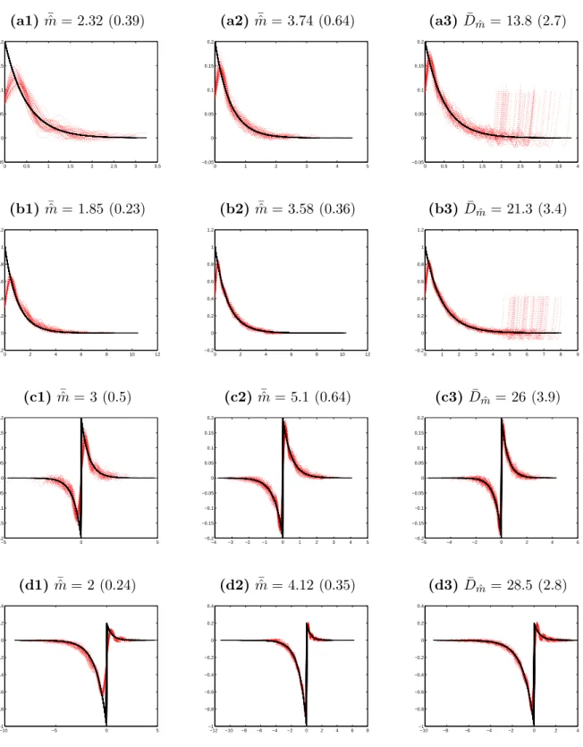
n(x) =|x|−1(βe−αx1I(0,+∞)(x) +β0e−α|x|1I(−∞,0)(x)). Rates are given in Table (2).
Process Example 2 Ex.2 (continued) Example 3
δ∈]0,1/2[ (continued) g∗(x) = β α−ix c Γ(δ+ 1/2) (β−iu)δ+1/2 β α−ix− β0 α0−ix R
|x|≥πm|g∗(x)|2dx= O(1/m) O(1/m2δ) O(1/m)
R
|x|≤πmnx
2|g∗(x)|2dx= O(m
n) O(m2n−2δ) O(mn)
Constraint on ∆ n∆2≤1 n∆2 ≤1 n∆2 ≤1
Selected m= O((n∆)1/2) O((n∆)1/(2δ+1)) O((n∆)1/2) Rate (small ∆) O((n∆)−1/2) O((n∆)−2δ/(2δ+1)) O((n∆)−1/2)
Rate (fixed ∆) O((n∆)−1/(2β∆+1)) O([ln(n∆)]−2δ) O((n∆)−1/(4β∆+1)) (see [5] (2008))
Table 2. Choice ofm and rates in examples 2, 2 (continued), 3 (continued).
The rates of the last lime in Table 2 come from Comte and Genon-Catalot (2008). As announced before (see Remark 3.2), the rates for small ∆ are different from the rates with fixed ∆, and they are in all cases better. Moreover, the estimation strategy in simpler and more complete (see Remark 4.2 in Comte and Genon-Catalot (2008)). The price to pay is the constraint on ∆.
5.2. Rates for the estimation on a compact set. In all the examples above, it is possible to find a compact setA such thatg is of class C∞on A.
Due to Corollary 4.1, for allα >0,E(kg−˜gm˜k2
A) =O((n∆)−2α/(2α+1)).
For the conditions under which this rate arises, three possibilities happen:
(1) for the compound Poisson process with Gaussian and exponential density, we have
R
u2|g∗(u)|2du <+∞,
(2) for the compound Poisson process with uniform densityf, the L´evy Gamma process and the bilateral L´evy Gamma process, we have R
u2|g∗(u)|2du= +∞ and g is bounded.
(3) For the L´evy-δ(see Example 2 (continued)), R
Choosing ∆ = n−a (see Corollary 4.1), in the first case, the best rate corresponding to
α→ +∞ is of orderO(n−2/3), for the second case, of order O(n−2/5) and for the third case of order O(n−1/3).
To conclude this section we show in Table 3 the best rate that can be obtained on each example according to the method, either Fourier method (Sinus Cardinal basis) or the time domain method (Trigonometric basis). The winner of the challenge is always the trigonometric basis. This is because the limit α → +∞ is considered for the latter basis only. However, on simulations, the global method performs better.
Process Sinus Cardinal basis Trigonometric basis Poisson-Gaussian ln1/2(n)n−2/3 n−2/3 Poisson-Exp. n−1/2 n−2/3 Poisson-Unif. n−1/4 n−2/5 L´evy-Gamma n−1/4 n−2/5 L´evy-δ n−δ/(2δ+1), δ ∈(0,1/2) n−1/3 Bilateral Gamma n−1/4 n−2/5
Table 3. Comparison of best possible rates with the two methods.
In all cases, rates measured as powers of n are very slow. As will be illustrated in the simulations, the important value isn∆, that should be large enough. This means that ∆ cannot be too small in order to keep a reasonable number n of observations. This is why, in our simulations, we have not always taken ∆2 smaller that 1/(n∆).
6. Simulations
We provide in this section simulation results. We have implemented the estimation method for two bases: the sinus cardinal basis of Section 3 and the trigonometric basis of Section 4. We simulated L´evy processes chosen among the examples given in Section 5. Precisely,
(1) A compound Poisson process with GaussianN(0,1) Yi’s,g(x) =cxexp(−x2/2)/
√
2π. (2) A compound Poisson process with Exponential E(1)Yi’s,g(x) =cxe−x1Ix>0.
(3) A compound Poisson process with Uniform U([0,1])Yi’s,g(x) =cx1I[0,1](x).
(4) A L´evy-Gamma process with parameters (α, β) = (2,0.2), g(x) =βexp(−αx)1Ix>0,
(5) A L´evy-Gamma process with parameters (α, β) = (1,1),
(6) A Bilateral L´evy-Gamma process with parameters (α, β) = (α0, β0) = (2,0.2), g(x) = βexp(−αx)1Ix≥0−β0exp(α0x)1Ix<0,
(7) A Bilateral L´evy-Gamma process with parameters (α, β) = (2,0.2) and (α0, β0) = (1,1)
After preliminary experiments, the constant κ is taken equal to 7.5 for the sinus cardinal basis and to 1 for the trigonometric basis. The cutoff ˆm is chosen among 100 equispaced values between 0 and 10. The dimensionDm˜ is chosen among 80 values between 1 and 80. We used
in both cases the expression of the estimators using the coefficients on the basis. In the sinus cardinal case, this avoids high dimensional matrices manipulations, but the series have to be truncated (we keep coefficients ˆam,j for|j| ≤Kn and we takeKn= 15).
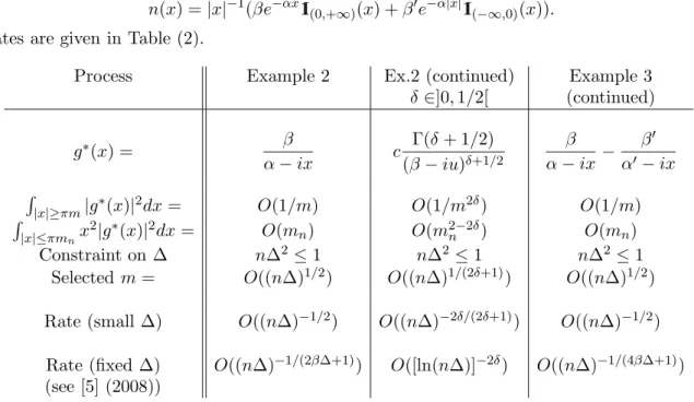
Results are given in Figures 1 and 2. We give confidence bands for our estimators by plotting 50 estimated curves on the same figure. The first two columns give estimation results with the sinus cardinal basis forn= 5000,∆ = 0.2 (n∆ = 1000) and n= 50000,∆ = 0.05 (n∆ = 2500). The third columns concerns the trigonometric basis forn= 50000,∆ = 0.05.
It is clear from the first two columns that increasingn∆ improves the result by showing a thin-ner confidence band. Comparing the last two columns amounts to comparing the performance of the two bases. It appears that the sinus cardinal must be preferred because the trigonometric basis has very important edge effects for highly dissymmetric densities: see in particular the exponential-Poisson, and the Gamma case, which start with a peak and end at zero.
On top of each graph in Figures 1 and 2, we give the mean of the selected values for ˆm (sinus cardinal basis) or for Dm˜ (trigonometric basis) with the associated standard deviation
in parentheses. Various values are chosen by the estimation procedure, and in each case, the standard deviation exhibits a reasonable variability. This is an indication that the constants in the penalties are adequately chosen: too small constants κ imply very unstable choices for the same model, while greaterκ’s quickly lead to null standard deviations for 50 sample paths. Note also that the higher the regularity ofg, the smaller the selected ˆm’s andDm˜’s (which is coherent
with orders asDm˜ =O(n1/(2α+1)) for a regularityα). The uniform-Poisson case involves larger
values for ˆm than the two other Poisson cases, for instance. At last, let us remark that, when R
u2|g∗(u)|2du <+∞, we need not use a C1-basis in the
second approach. For instance, a histogram basis or a piecewise polynomial basis can also be implemented. But in practice, it is not possible to know if the condition is fulfilled or not.
7. Concluding remarks
In this paper, we have investigated in the high frequency framework the nonparametric es-timation of the L´evy density n(·) of a pure jump L´evy process under assumption (H1). This paper complements a previous one (Comte and Genon-Catalot (2008)) where the low frequency framework was treated. The estimation of n(.) is done through the estimation of the function g(x) = xn(x). In here, we use two kinds of bases. On the one hand, the sinus cardinal basis, which is of classical use in deconvolution provides a global estimation. On the other hand, finite dimensional bases satisfying (21) provide an estimation ofgrestricted to a compact set. In each approach, an adaptive estimator is built which reaches automatically the classical best rate that can be achieved on a prescribed class of regularity. The estimators can easily be implemented. Especially in the case of the sinus cardinal basis, the method allows the automatic (and adap-tive) choice of a cutoff valuemin Fourier inversion, a point that was unsolved in several previous references (quoted in the introduction).
There remain several open problems: mainly, how can the method be extended to more general L´evy processes having a drift term and under a weaker assumption on n(·) such as
R
x2n(x)dx <+∞ (see Neumann and Reiss (2009)).
8. Appendix: Proofs
8.1. Proof of Theorem 2.1. We apply Rosenthal’s inequality recalled in Appendix (see (51)): E 1 n n X k=1 Zk`−E(Z1`) p! ≤ C(p)np n X k=1 E[|Zk`−E(Z1`)|p] + n X k=1 E[(Zk`−E(Z1`))2] !p/2 ≤ C(p)np (nE[|Z1`−E(Z1`)|p] +np/2(E[(Z1`−E(Z1`))2])p/2) ≤ Cn0(p)p (nE(Zp` 1 ) +np/2[E(Z12`)]p/2) ≤ C”(p) ∆ np−1 + ∆ n p/2! .
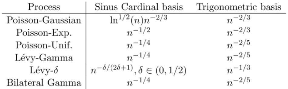
(a1)m¯ˆ = 0.85 (0.05) (a2) m¯ˆ = 0.91 (0.03.) (a3) D¯mˆ = 5.08 (0.34) −6 −4 −2 0 2 4 6 −0.2 −0.15 −0.1 −0.05 0 0.05 0.1 0.15 −5 0 5 −0.2 −0.15 −0.1 −0.05 0 0.05 0.1 0.15 −5 0 5 −0.2 −0.15 −0.1 −0.05 0 0.05 0.1 0.15 (b1) m¯ˆ = 0.7 (0.09) (b2) m¯ˆ = 0.88 (0.08) (b3) D¯mˆ = 4.8 (0.90) 0 2 4 6 8 10 12 −0.05 0 0.05 0.1 0.15 0.2 0 2 4 6 8 10 12 14 −0.05 0 0.05 0.1 0.15 0.2 0 2 4 6 8 10 12 −0.05 0 0.05 0.1 0.15 0.2 (c1) m¯ˆ = 3.0 (0.66) (c2)m¯ˆ = 5.26 (0.89) (c3)D¯mˆ = 15.4 (4.9) 0 0.5 1 1.5 2 2.5 3 −0.1 0 0.1 0.2 0.3 0.4 0.5 0.6 0 0.5 1 1.5 2 −0.1 0 0.1 0.2 0.3 0.4 0.5 0.6 0 0.5 1 1.5 2 2.5 −0.1 0 0.1 0.2 0.3 0.4 0.5 0.6 0.7
Figure 1. Confidence band for the estimation of g for a compound Poisson
process with Gaussian (first line), Exponential E(1) (second line), and uniform
U([0,1]) (third line)Yi’s,c= 0.5. True (bold black line) and 50 estimated curves
(dotted red), left ∆ = 0.2 n = 5000, Sinus Cardinal Basis; center, ∆ = 0.05, n= 5.104, Sinus Cardinal Basis; right ∆ = 0.05,n= 5.104, trigonometric basis.
We have 1 n∆ n X k=1 Zk`−m`= 1 n∆ n X k=1 (Zk`−E(Z` 1) ! + 1 ∆E(Z ` 1)−m`.
First note that, by Proposition 2.2, 1 ∆E(Z
`
1)−m`= ∆O(1).
(a1)m¯ˆ = 2.32 (0.39) (a2) m¯ˆ = 3.74 (0.64) (a3) D¯mˆ = 13.8 (2.7) 0 0.5 1 1.5 2 2.5 3 3.5 −0.05 0 0.05 0.1 0.15 0.2 0 1 2 3 4 5 −0.05 0 0.05 0.1 0.15 0.2 0 0.5 1 1.5 2 2.5 3 3.5 4 −0.05 0 0.05 0.1 0.15 0.2 (b1) m¯ˆ = 1.85 (0.23) (b2) m¯ˆ = 3.58 (0.36) (b3) D¯mˆ = 21.3 (3.4) 0 2 4 6 8 10 12 −0.2 0 0.2 0.4 0.6 0.8 1 1.2 0 2 4 6 8 10 12 −0.2 0 0.2 0.4 0.6 0.8 1 1.2 0 1 2 3 4 5 6 7 8 9 −0.2 0 0.2 0.4 0.6 0.8 1 1.2 (c1)m¯ˆ = 3 (0.5) (c2)m¯ˆ = 5.1 (0.64) (c3) D¯mˆ = 26 (3.9) −5 0 5 −0.2 −0.15 −0.1 −0.05 0 0.05 0.1 0.15 0.2 −4 −3 −2 −1 0 1 2 3 4 5 −0.2 −0.15 −0.1 −0.05 0 0.05 0.1 0.15 0.2 −6 −4 −2 0 2 4 6 −0.2 −0.15 −0.1 −0.05 0 0.05 0.1 0.15 0.2 (d1) m¯ˆ = 2 (0.24) (d2) m¯ˆ = 4.12 (0.35) (d3) D¯mˆ = 28.5 (2.8) −10 −5 0 5 −1 −0.8 −0.6 −0.4 −0.2 0 0.2 0.4 −12 −10 −8 −6 −4 −2 0 2 4 6 8 −1 −0.8 −0.6 −0.4 −0.2 0 0.2 0.4 −10 −8 −6 −4 −2 0 2 4 −1 −0.8 −0.6 −0.4 −0.2 0 0.2 0.4
Figure 2. Confidence band for the estimation of g for a L´evy Gamma process
with parameters (α, β) = (2,0.2) (first line), (α, β) = (1,1) (second line), a bilateral L´evy Gamma process with parameters (α, β) = (α0, β0) = (2,0.2) (third line) and a bilateral L´evy Gamma process with parameters (α, β) = (2,0.2), (α0, β0) = (1,1). True (bold black line) and 50 estimated curves (dotted red), left ∆ = 0.2 n= 5000, Sinus Cardinal Basis; center, ∆ = 0.05, n= 5.104, Sinus
Let us introduce the centered i.i.d. random variables ξk= 1 √ n∆(Z ` k−E(Z1`)). We have nE(ξ2 k) = 1 ∆(E(Z 2` k )−(E(Z1`))2) =m2`+o(1). And nE(ξ4k)≤Cn 1 n2∆2(E(Z 4` k ) + (E(Z1`)4)) = 1 n∆(m4`+O(1)), which tends to 0. Hence, the result.
8.2. Proof of Proposition 2.3. By the Taylor formula, ψ∆(u)−1 =uψ
0
∆(cuu) =iu∆ψ∆(cuu)g∗(cuu),
for somecu ∈(0,1). This gives (10) and thus (11).
For the other bound withp= 1, note that
E(|θˆ∆(u)−θ∆(u)|2) = 1
nVar(Z1exp (iuZ1))≤ 1 nE(Z
2 1).
Inequality (13)follows.
Forp≥1, we apply Rosenthal’s inequality recalled in Appendix (see (51)):
E E(|θˆ∆(u)))−θ∆(u)|2p) ≤ C(2p)n2p n X k=1 E[|ZkeiuZk −E(Z keiuZk)|2p] + n X k=1 E|ZkeiuZk−E(Z keiuZk)|2] !p! ≤ C0(2p) n2p (nE(Z 2p 1 ) +np(E(Z12))p).
We conclude using Proposition 2.2 and p≥1.
8.3. Proof of Theorem 2.2. We have
√ n∆(ˆθ∆(u)/∆−g∗(u)) = √ n∆ θˆ∆(u)−θ∆(u) ∆ +g ∗(u)(ψ ∆(u)−1) ! . Hence, the bias term in √n∆(ˆθ∆(u)/∆−g∗(u)) is of order
√
n∆∆ =√n∆3. This explains the
condition n∆3 = o(1) in Theorem 2.2. There remains to study Xn(u) =
√ n∆(∆−1θˆ∆(u) − ∆−1θ∆(u)). Using (5), we have, Xn(u) = Z eiux√n∆(ˆµn(dx)−µ∆(dx)) = n X k=1 Xk,n(u), with Xk,n(u) = 1 √ n∆(Zke iuZk −θ ∆(u)).
Consider, for any integer l≥1,u1, u2, . . . , ul∈R. We need to prove that the random vector
Xn = (Xn(u1), Xn(u2), . . . , Xn(ul))0 (with values in Cl) converges in distribution to Nl(0, V)
where the covariance matrix V is given by: Vj,j0 =
Z
Let us set g1=gand for `≥1,
(34) g`(x) =x`−1g(x) =x`n(x).
Since the random variables Xk,n(u) are independent, identically distributed and centered, it
is enough to check that, for all (u, v)
(35) nE(Xk,n(u) ¯Xk,n(v))→V(u, v) = Z ei(u−v)xx2n(x)dx=g∗2(u−v), and (36) nE(|Xk,n(u)|4)→0. We have: nE(Xk,n(u) ¯Xk,n(v)) = 1 ∆(E(Z 2 kei(u−v)Zk)−θ∆(u)¯θ∆(v)) and E(Z2 1ei(u−v)Z1) =−ψ 00 ∆(u−v)). Computingψ∆00, we get:
ψ∆00(u) =−∆ψ∆(u)[g2∗(u) + ∆(g∗(u))2].
Since θ∆(u)¯θ∆(v) = ∆2g∗(u)g∗(−v)ψ∆(u)ψ∆(−v),
nE(Xk,n(u) ¯Xk,n(v)) =ψ∆(u−v)[g2∗(u−v) + ∆O(1)] =g2∗(u−v) +o(1), which gives (35). Moreover, (37) nE(|Xk,n(u)|4)≤ 8 n∆2(E(Z 4 k) +|θ∆(u)|4) = 8 n∆(m4+o(1)), which implies (36).
8.4. Proof of Theorem 3.1. The proof is given in two steps. We define, for someb, 0< b <1, Ωb:= (1/n∆)Pn k=1Zk2 E(Z2 1/∆) −1 ≤ b , so that E(kˆgmˆ −gk2) =E(kˆgmˆ −gk21IΩ b) +E(kgˆmˆ −gk 21I Ωc b). Step 1. Study ofE(kˆgmˆ −gk21IΩ
b). For notational convenience, let us define, fort∈Sm:
(38) νn(t) = 1 2π Z ˆ θ∆(u)−θ∆(u) ∆ t ∗(−u)du (39) Rn(t) = 1 2π Z
(ψ∆(u)−1)g∗(u)t∗(−u)du.
We have used the same notation as in (25) and (26) but the interpretation is different. Note thatνn= ¯νn and Rn= ¯Rn so that they are both real valued. Then (24) holds.
We must splitνn into two terms. Withkn to be defined later on, let
θ(1)∆ (x) =E Z11I|Z1|≤kn√∆eixZ1 and θ∆(2)(x) =E Z11I|Z1|>kn√∆eixZ1
and ˆθ(1)∆ (x) and ˆθ∆(2)(x) their empirical counterparts. We define νn(1)(t) = 1
2π∆
Z
and
νn(2)(t) = 1 2π∆
Z
(ˆθ∆(2)(u)−θ∆(2)(u))t∗(−u)du. The definition of ˆgmˆ implies that
(40) γn(ˆgmˆ) + pen( ˆm)≤γn(gm) + pen(m)
wheregm denotes the orthogonal projection of g on Sm.
Then, using (24) yields that, for allm= 1, . . . , mn,
kˆgmˆ −gk2 ≤ kg−gmk2+ pen(m) + 2νn(1)(gm−ˆgmˆ)−pen( ˆm) +2Rn(gm−ˆgmˆ) + 2νn(2)(gm−gˆmˆ) ≤ kg−gmk2+ pen(m) + 3 8kgm−gˆmˆk 2+ 8 sup t∈Sm+Smˆ,ktk=1 [νn(1)(t)]2−pen( ˆm) +8 sup t∈Smn,ktk=1 [Rn(t)]2+ 8 sup t∈Smn,ktk=1 [νn(2)(t)]2 ≤ (1 +3 4)kg−gmk 2+ pen(m) +3 4kgˆmˆ −gk 2 +8 sup t∈Sm+Smˆ,ktk=1 [νn(1)(t)]2−p(m,m)ˆ ! + + 8p(m,m)ˆ −pen( ˆm) +8 sup t∈Smn,ktk=1 [Rn(t)]2+ 8 sup t∈Smn,ktk=1 [νn(2)(t)]2.
The functionp(m, m0) plugged in the last inequality is fixed by applying Talagrand’s inequality (see Lemma 9.1) to νn(1), which yields the following result:
Proposition 8.1. Under the Assumptions of Theorem 3.1, define
(41) p(m, m0) = 4E(Z2 1/∆) m∨m0 n∆ , then E( sup t∈Sm+Smˆ,ktk=1 [νn(1)(t)]2−p(m,m))ˆ + ≤ mn X m0=1 E( sup t∈Sm+Sm0,ktk=1 [νn(1)(t)]2−p(m, m0))+≤ C n∆, where C is a constant.
Now, on Ωb, the following inequality holds (by bounding the indicator by 1), for any choice
of κ:
(42) ∀m, (1−b)penth(m)≤pen(m)≤(1 +b)penth(m).
Therefore 1 4kˆgmˆ −gk 21I Ωb ≤ 7 4kg−gmk 2+ (1 +b)pen th(m)1IΩb+ 8 sup t∈Sm+Smˆ,ktk=1 [νn(1)(t)]2−p(m,m)ˆ ! + +(8p(m,m)ˆ −(1−b)penth( ˆm))1IΩb +8 sup t∈Smn,ktk=1 [Rn(t)]2+ 8 sup t∈Smn,ktk=1 [νn(2)(t)]2. The constant κis now chosen such that
that is κ≥32/(1−b). In view of (41), this gives the choices penth(m) = 32 1−bE(Z 2 1/∆) m n∆ and pen(m) = 32 1−b 1 n∆ n X i=1 Zi2 m n∆. It follows that 1 4kˆgmˆ −gk 21I Ωb ≤ 7 4kg−gmk 2+ 2pen th(m) +8 mn X m0=1 sup t∈Sm+Sm0,ktk=1 [νn(1)(t)]2−p(m, m0) ! + +8 sup t∈Smn,ktk=1 [Rn(t)]2+ 8 sup t∈Smn,ktk=1 [νn(2)(t)]2. Using (39) and (10), we get
(43) sup t∈Smn,ktk=1 R2n(t)≤C∆2 Z πmn −πmn u2|g∗(u)|2du. Forνn(2)(t), we write E sup t∈Smn,ktk=1 [νn(2)(t)]2 ! ≤ 1 2π∆2 Z πmn −πmn E|θˆ(2) ∆ (u)−θ (2) ∆ (u)|2du ≤ E(Z2 11I|Z1|>kn√∆)mn n∆2 ≤ E(Z 4 1)mn nk2 n∆3 = [E(Z 4 1)/∆]mn nk2 n∆2 ≤ [E(Z4 1)/∆] k2 n∆
since mn ≤ n∆. We know that [E(Z14)/∆] is bounded. If kn2 ≥ Cn/ln2(n∆), then the above
term is of order ln2(n∆)/(n∆) .
Then we obtain that, for allm∈ {1, . . . , mn},
E kgˆmˆ −gk21IΩ b ≤7kg−gmk2+ 8penth(m) + C1 n∆+C2∆ 2Z πmn −πmn u2|g∗(u)|2du+C3 ln2(n∆) n∆ . Step 2. Study ofE(kˆgmˆ −gk21IΩc b).
The strategy is different. Using (24) and (40) yields that,∀m∈ {1, . . . , mn},
kgˆmˆ −gk2 ≤ kg−gmk2+ pen(m) + 2νn(gm−ˆgmˆ)−pen( ˆm) + 2Rn(gm−gˆmˆ) ≤ kg−gmk2+ pen(m) + 1 4kgm−ˆgmˆk 2 (44) +8 sup t∈Smn,ktk=1 [νn(t)]2+ 8 sup t∈Smn,ktk=1 [Rn(t)]2. (45)
Now we apply inequality (43) to Rn(t) and the Parseval formula for νn(t), and get
1 2kgˆmˆ −gk 2 ≤ 3 2kg−gmk 2+ pen th(m) + [pen(m)−E(pen(m))] + 4 π∆2 Z πmn −πmn |θˆ∆(u)−θ∆(u)|2du+C0∆2 Z πmn −πmn u2|g∗(u)|2du.
Therefore, using that penth(m) =E(pen(m)), we obtain (46) E (pen(m)−penth(m))1IΩc
b ≤ E 1 n∆ n X k=1 (Zk2−E(Z2 1) !2 1/2 (P(Ωc b))1/2, and we find 1 2E(kgˆmˆ −gk 21I Ωc b) ≤ 3 2kgk 2+ pen th(m) +C”∆2m2nkgk2 P(Ωc b) +E1/2 1 n∆ n X k=1 (Zk2−E(Z12) !2 P1/2(Ωcb) +E1/2 ( 4 π∆2 Z πmn −πmn
|θˆ∆(u)−θ∆(u)|2du)2
P1/2(Ωc
b).
Then we apply (9) of Theorem 2.1 with `= 2 and get forp≥2:
E 1 n∆ n X k=1 Zk2−E(Z12) p! ≤Cp 1 n∆ p/2 . Thus, by takingp= 2, E1/2 ( 1 n∆ n X i=1 (Zi2−E(Zi2))2 ! ≤ √C n∆. Applying (12) forp= 2 gives
E(|θˆ∆(u)−θ∆(u)|4)≤ C∆ 2 n2 . Thus E ( 4 π∆2 Z πmn −πmn
|θˆ∆(u)−θ∆(u)|2du)2
≤ π162∆4(2πmn)
Z πmn
−πmn
E(|θˆ∆(u)−θ∆(u)|4du)
≤ C0m 2 n ∆4 ∆2 n2 ≤C0 asmn≤n∆. We obtain: (47) E(kˆgmˆ −gk21IΩc b)≤C 1 +n 2∆4 P(Ωc b) +C0(1 + 1 √ n∆)P 1/2(Ωc b).
Lastly, if follows from the Markov inequality that
P(Ωc b) ≤ 1 bpE (1/n∆)Pn k=1Zk2 E(Z2 1/∆) −1 p ≤ 1 (E(Z2 1/∆)b)p E 1 n∆ n X k=1 Zi2−E(Z12/∆) p! . We find that, ifE(|Z1|2p)<+∞ andp≥2,
(48) P(Ωc b)≤ Cp (E(Z2 1/∆)b)p 1 (n∆)p/2.
Therefore, using (47) and the above inequality, if we takep= 4 (i.e. E(Z8
1)<∞), we get
E(kgˆmˆ −gk21IΩc
This ends step 2 and the proof of Theorem 3.1.
8.5. Proof of Proposition 8.1. Here we apply the Talagrand (see Lemma 9.1) Inequality to the class F ={ft, t∈Sm+Sm0} whereft(z) = z1I|z|≤k n √ ∆ 2π∆ Z π(m∨m0) −π(m∨m0) eixzt∗(−x)dx.
In that case,νn(1)(t) = (1/n)Pnk=1(ft(Zk)−E(ft(Zk))).We have to find the three quantitiesM,
H,v.
Letm” =m∨m0, and note thatSm+Sm0 =Sm”. Using Inequality (17),
sup z∈R| ft(z)| ≤ kn 2π√∆supz∈R| 2πt(z)| ≤ kn√ktk∞ ∆ ≤ kn √ m” √ ∆ :=M. Clearly, E sup t∈Sm+Sm0,ktk=1 [νn(1)(t)]2 ! ≤ 1 2π∆2 Z πm” −πm” E|θˆ(1) ∆ (u)−θ (1) ∆ (u)|2du≤ E(Z2 1)m” n∆2 . Thus we set H2 = E(Z 2 1)m” n∆2 .
The most delicate term isv. Var(ft(Z1)) ≤ 1 4π2∆2E Z Z Z121I|Z 1|≤kn√∆e i(x−y)Z1t∗(−x)t∗(y)dxdy = 1 4π2∆2 Z Z p∗∆(x−y)t∗(−x)t∗(y)dxdy, where p∗∆(x) =E(Z121I |Z1|≤kn√∆e ixZ1). Using thatt=P j∈Ztjϕm”,j withktk2 = P j∈Zt2j = 1, Var(ft(Z1)) ≤ 1 4π2∆2 X j,k∈Z tjtk Z Z p∗∆(x−y)ϕ∗m”,j(−x)ϕ∗m”,k(y)dxdy ≤ 1 4π2∆2 X j,k∈Z Z Z p∗∆(x−y)ϕ∗m”,j(−x)ϕ∗m”,k(y)dxdy 2 1/2 , Now, using Proposition 2.1, we have
p∗∆(x) = ∆ Z z1I|z|≤k n√∆e ixzE(g(z−Z 1))dz.
This implies that (see (H4))
Z |p∗∆(z)|2dz ≤ 2π Z |p∆(z)|2dz = 2π∆2 Z z21I|z|≤kn√ ∆E2(g(z−Z1))dz ≤ 2π∆2E Z z21I|z|≤k n √ ∆g 2(z−Z 1)dz ≤ 4π∆2E Z (x2+Z12)g2(x)dx = 4π∆2 M2+E(Z12)kgk2 .
Therefore, it follows Var(ft(Z1)) ≤ 1 4π2∆2 Z Z [−πm”,πm”]2| p∗∆(x−y)|2dxdy !1/2 ≤ 4π21∆2(2πm”)1/2( Z |p∗∆(z)|2dz)1/2 ≤ √ m” √ 2π∆ M2+kgk 2E(Z2 1) 1/2 :=v. Applying Lemma 9.1 yields, for2 = 1/2 and p(m, m0) given by (41) yields
E sup t∈Sm+Sm0,ktk=1 [νn(1)(t)]2−p(m, m0) ! + ≤C1 √ m” n∆ e −C2√m”+k 2 nm” n2∆ e− C3√n/kn ! asp(m, m0) = 4H2. We choose kn= C3 4 √ n ln(n∆), and as m≤n∆, we get E sup t∈Sm+Sm0,ktk=1 [νn(1)(t)]2−p(m, m0) ! + ≤C10 √ m” n∆ e− C2√m”+ 1 (∆n)4ln2(n∆) ! . Therefore mn X m0=1 E sup t∈Sm+Sm0,ktk=1 [νn(1)(t)]2−p(m, m0) ! + ≤C10 Pn∆ m0=1 √ m”e−C2√m” n∆ + 1 (n∆)3ln2(n∆) ! . AsC2xe−C2x is decreasing for x≥1/C2, and its maximum is 1/(eC2), we get
mn X m0=1 √ m”e−C2√m” ≤ X √ m0≤1/C2 (eC2)−1+ X √ m0≥1/C2 √ m0e−C2√m0 ≤ 1 eC3 2 + ∞ X m0=1 √ m0e−C2√m0 <+∞. I follows that mn X m0=1 E sup t∈Sm+Sm0,ktk=1 [νn(1)(t)]2−p(m, m0) ! + ≤ n∆C
and Proposition 8.1 is proved.
8.6. Proof of Proposition 4.1. First, we know that Rn(t) = (1/2π)
R
(ψ∆−1)g∗(u)t∗(−u)
and thus, ifR
u2|g∗(u)|du <+∞, if follows from (10) that
R2n(t)≤ ∆ 2kgk2 1 (2π)2 Z |ug∗(u)t∗(−u)|du 2 ≤ ∆ 2kgk2 1 (2π)2 Z u2|g∗(u)|2du Z |t∗(−u)|2du. Noting that R |t∗(−u)|2du= 2πktk2 = 2πktk2 A gives 1).
For the two other cases, using Proposition 2.1, we have, forta function with support [a, b]: 1 ∆E(Z1t(Z1)) = Z b a t(z)Eg(z−Z1)dz=E( Z b−Z1 a−Z1 t(x+Z1)g(x)dx).
ThusRn(t) =E(
Rb−Z1
a−Z1 t(x+Z1)g(x)dx−
Rb
at(x)g(x)dx).
On (|Z1|> b−a), [a−Z1, b−Z1]∩[a, b] =∅ and
E 1I|Z1|>b−a Z b−Z1 a−Z1 t(x+Z1)g(x)dx− Z b a t(x)g(x)dx ≤ 2ktk∞kgk1 E(|Z1|) b−a ≤ 4Φ0kgk 2 1 √ Dm∆ktkA b−a .
On (|Z1| ≤b−a), [a−Z1, b−Z1]∩[a, b]6=∅. Assume for instance that 0≤Z1 ≤b−a.
Z b−Z1 a−Z1 t(x+Z1)g(x)dx− Z b a t(x)g(x)dx = Z a a−Z1 t(x+Z1)g(x)dx+ Z b−Z1 a (t(x+Z1)−t(x))g(x)dx− Z b b−Z1 t(x)g(x)dx. To study the middle term, we use the fact that tis C1 on [a, b].
T1 := E 1I0≤Z1≤b−a Z b−Z1 a (t(x+Z1)−t(x))g(x)dx = E Z11I0≤Z1≤b−a Z b−Z1 a Z 1 0 t0(x+uZ1)dug(x)dx = E Z11I0≤Z1≤b−a Z 1 0 ( Z b−Z1 a t0(x+uZ1)g(x)dx)du
An application of the Cauchy-Schwarz inequality yields
|T1| ≤E|Z1|kt0kAkgk ≤2Φ0kgk1kgkktkA∆Dm. Next, T2:=E 1I0≤Z1≤b−a Z a a−Z1 t(x+Z1)g(x)dx . Here we distinguish between 2) and 3). Ifg is bounded (case 2)), then
|T2| ≤ ktk∞kgk∞E(|Z1|)≤2Φ0kgk1ktkA∆
p
Dm.
Otherwise (case 3)), using the Cauchy-Schwarz inequality again,
|T2| ≤ E( q Z1+)ktk∞kgk ≤pE(|Z1|)Φ0pDmktkAkgk ≤ √2Φ0ktkA p kgk1kgk p Dm∆.
The same bound holds for the last term.
The same study can be done for a−b ≤ Z1 ≤ 0. Joining all terms, we find that, if g is
bounded |Rn(t)| ≤CΦ0ktkA∆Dm. Otherwise, |Rn(t)| ≤C0Φ0ktkA( p ∆Dm+ ∆Dm).
![Figure 1. Confidence band for the estimation of g for a compound Poisson process with Gaussian (first line), Exponential E(1) (second line), and uniform U([0, 1]) (third line) Y i ’s, c = 0.5](https://thumb-us.123doks.com/thumbv2/123dok_us/9484300.2823635/19.892.130.790.110.726/figure-confidence-estimation-compound-poisson-process-gaussian-exponential.webp)