www.elsevier.com/locate/jmva
Sparse principal component analysis via regularized
low rank matrix approximation
Haipeng Shen
a,∗, Jianhua Z. Huang
baDepartment of Statistics and Operations Research, University of North Carolina at Chapel Hill, Chapel Hill, NC
27599, USA
bDepartment of Statistics, Texas A&M University, College Station, TX 77843, USA Received 25 July 2006
Available online 27 June 2007
Abstract
Principal component analysis (PCA) is a widely used tool for data analysis and dimension reduction in applications throughout science and engineering. However, the principal components (PCs) can sometimes be difficult to interpret, because they are linear combinations of all the original variables. To facilitate interpretation, sparse PCA produces modified PCs with sparse loadings, i.e. loadings with very few non-zero elements. In this paper, we propose a new sparse PCA method, namelysparse PCA via regularized SVD
(sPCA-rSVD). We use the connection of PCA with singular value decomposition (SVD) of the data matrix and extract the PCs through solving a low rank matrix approximation problem. Regularization penalties are introduced to the corresponding minimization problem to promote sparsity in PC loadings. An efficient iterative algorithm is proposed for computation. Two tuning parameter selection methods are discussed. Some theoretical results are established to justify the use of sPCA-rSVD when only the data covariance matrix is available. In addition, we give a modified definition of variance explained by the sparse PCs. The sPCA-rSVD provides a uniform treatment of both classical multivariate data and high-dimension-low-sample-size (HDLSS) data. Further understanding of sPCA-rSVD and some existing alternatives is gained through simulation studies and real data examples, which suggests that sPCA-rSVD provides competitive results.
© 2007 Elsevier Inc. All rights reserved.
AMS 1991 subject classification:62H20; 62H25; 62H30
Keywords:Dimension reduction; High-dimension-low-sample-size; Regularization; Singular value decomposition; Thresholding
∗Corresponding author.
E-mail addresses:[email protected](H. Shen),[email protected](J.Z. Huang). 0047-259X/$ - see front matter © 2007 Elsevier Inc. All rights reserved.
1. Introduction
Principal component analysis (PCA) has been widely used in many applications as a feature extraction and dimension reduction tool as well illustrated in Jolliffe[11]. SupposeXis ann×p
data matrix with rank(X)= r, which recordspvariables onnobservations. PCA sequentially finds unit vectorsv1, . . . ,vr that maximize the variance ofXvunder the constraint thatvi+1is orthogonal tov1, . . . ,vi. Such vectors are called principal component (PC) loadings, and theXvi’s are the corresponding PCs. The idea of dimension reduction using PCA is that the firstfewPCs might retain most of the variation in the data. Interpretation of PCs is useful, especially when the variables have physical meanings, for example, in microarray data each variable corresponds to a specific gene. However, PCs are usually linear combinations ofallthe original variables and their loadings are typically non-zero. This often makes it difficult to interpret the PCs without using subjective judgment, especially whenpis large as frequently encountered in modern statistical applications.
To ease this drawback of PCA, various proposals have been introduced in the literature. Jol-liffe [10] described several rotation techniques that are helpful for interpreting PCs. JolJol-liffe and Uddin [13] proposed SCoT to successively find linear combinations that maximize a criterion which balances variance and some simplicity measure. Vines [17] consideredsimple compo-nents, whose loadings are restricted to only integers such as 0, 1 and −1. Another group of methods, referred to as sparsePCA methods, aims at finding loading vectors with many zero components, thus increasing interpretability of PCs by reducing the number of explicitly used variables. Cadima and Jolliffe [2] described asimple thresholdingapproach, which artificially sets regular PC loadings to zero if their absolute values are below a certain threshold. Jolliffe et al. [12] proposed SCoTLASS, which applies thelassopenalty [16] on the loadings in a PCA op-timization problem. More recently, Zou et al. [20] reformulated PCA as a regression-type problem, and proposed SPCA which achieves sparseness by imposing the lasso penalty on the regression coefficients.
In this paper, we provide a new approach to achieve sparse PCA, making use of the close connection between PCA and singular value decomposition (SVD) that PCA can be computed via the SVD of the data matrix X. Without loss of generality, assume the columns of Xare centered. Suppose rank(X)=rand let the SVD ofXbe
X=UDVT,
whereU = [u1, . . . ,ur],V = [v1, . . . ,vr]andD = diag{d1, . . . , dr}. The columns ofUare
orthonormal, so are the columns ofV. The singular values are assumed to be ordered so that
d1d2· · ·dr >0. Then, the columns ofZ=UDare the PCs, and the columns ofVare the
corresponding loadings.
To motivate our approach, we need to look at SVD from the viewpoint of low rank approximation of matrices. For an integerlr, define
X(l)≡ l
k=1
dkukvTk.
Then,X(l) is the closest rank-lmatrix approximation to X[4]. Here the term “closest” simply means thatX(l)minimizes the squared Frobenius norm betweenXand an arbitrary rank-lmatrix
X∗, where the Frobenius norm is defined as
X−X∗2F =tr{(X−X∗)(X−X∗)T}.
Suppose, for example, we seek the best rank-one matrix approximation ofXunder the Frobenius norm. Note that anyn×prank-one matrix can be written asuvT, whereuis a norm-1n-vector andvis ap-vector. The problem can be formulated as the following optimization problem:
minu,vX−uvT2F. (1)
Then the low rank approximation property of SVD implies that the solution is
u=u1, v=d1v1.
The subsequent pairs(uk, dkvk),k >1, provide best rank one approximations of the
correspond-ing residual matrices. For example,d2u2vT2 is the best rank one approximation ofX−d1u1vT1. To obtain sparse loadings, we impose regularization penalties onvin the optimization problem (1), and refer to our approach as sparse PCA via regularized SVD, or sPCA-rSVD for short. The key of our proposal is the observation that the optimization problem (1) is connected to least squares regressions. For a fixedu, the optimalvis the least squares coefficient vector of regressing the columns ofXonu. Introducing sparsity onvin such a context is a familiar variable selection problem in regression. Thus many existing variable selection techniques using regularization penalties [16,3,5] are readily applicable.
The benefit of imposing sparsity-inducing penalties onvin the optimization (1) is two-fold. First, the resulting PC loading vector is made sparse so that thosenegligiblevariables will not appear in the corresponding PC, therefore the PCs obtained are more interpretable. Meanwhile, since the left-out variables arenegligible, the sparse PC won’t suffer much in terms of the variance it explains. Second, when a covariance matrix has sparse eigenvectors, by using the sparsity-inducing penalties, sPCA-rSVD is statistically more efficient than the standard PCA in extracting the PCs, as illustrated using simulated examples in Sections 3.2 and 3.3. This is similar to regression problems with irrelevant regressors, where variable selection improves statistical efficiency.
We propose an iterative algorithm for computation of sPCA-rSVD. The algorithm only involves simple linear regression and componentwise thresholding rules; hence it enjoys nice properties such as easy implementation and efficient computation. We define thedegree of sparsityof a PC as the number of zero components in the corresponding loading vector. The degree of sparsity naturally serves as the tuning parameter of the method. Two approaches are proposed to select the “optimal” degree of sparsity, one cross validation approach, and one ad hoc approach that is useful when the sample size is small or only the data covariance matrix is available. Different degree of sparsity is allowed for different loading vectors in our framework.
In addition to proposing sPCA-rSVD, we give a new definition of variance explained by the sparse PCs. This is necessary since for sparse PCA, the loading vectors need not be orthogonal and the PCs need not be uncorrelated, which makes the conventional definition too optimistic. We fix the problem of the conventional definition by using the viewpoint of dimension reduction. Our definition of the variance explained by the sparse PCs can be used to select the tuning parameters specifying sparsity, or to select the number of important PCs.
In this paper, we also prove that our sPCA-rSVD procedure still applies when only the co-variance matrix is available, because it depends on the data through the Gram matrixXTX. The sPCA-rSVD handles both “long” data matrices wherenpand “fat” matrices wheren < por evenn>pin a unified way. Standard PCA in classical multivariate analysis usually deals with
the “long” data matrices. The “fat” matrices arehigh-dimension-low-sample-size(HDLSS) data objects[15]. HDLSS has rapidly become a common feature of data encountered in many diverse fields such as text categorization, medical imaging and microarray gene expression analysis, and is outside the domain of classical multivariate analysis.
The rest of the paper is organized as follows. We present the methodological details of our sPCA-rSVD procedure in Section 2. Section 2.1 gives the optimization criterion that leads to sparse PCA; Section 2.2 describes an efficient iterative algorithm for computation; Section 2.3 proposes a modified definition of the variance explained by the sparse PCs; Section 2.4 discusses extraction of sparse PC loadings when only the covariance matrix of the data is available; Section 2.5 provides methods for tuning parameter selection. Further understanding of the proposed method, mainly through simulation studies, is provided in Section 3. Sections 4 and 5 compare the proposed procedure with SPCA and simple thresholding, respectively. Section 6 illustrates the proposed method using some real data examples. We end the paper with some discussion in Section 7 and technical proofs in Appendix A.
2. Sparse PCA via regularized SVD
This section describes in detail our sPCA-rSVD procedure. We focus our presentation on the procedure extracting the first sparse PC loading vector. Subsequent loading vectors can be obtained by applying the same procedure to the residual matrices of the sequential matrix approximations.
2.1. A penalized sum-of-squares criterion
SupposeuvT withv = 1 is the best rank-one approximation of the data matrixX. Then
uis the first PC andvis the corresponding loading vector. For a givenu, elements ofvare the regression coefficients by regressing the columns ofXon u. To achieve sparseness onv, we propose to employ some regularization penalties in these regressions that promote shrinkage and sparsity on the regression coefficients.
However, the loading vectorv is typically constrained to have unit length to make the rep-resentation unique. This constraint makes direct application of a penalty onvinappropriate. To overcome this difficulty, we rewriteuvT =uvT, whereuandvare re-scaled versions ofuandv
such thatuhas unit length andvis free of any scale constraint, and then perform shrinkage on vthrough some regularization penalty. After a sparsevis obtained, we define the corresponding
sparse loading vector asv=v/v.
The precise formulation of our idea is the following. For a givenn×pdata matrixX, we find an
n-vectoruwithu =1 and ap-vectorvthat minimize the following penalized sum-of-squares criterion, X−uvT2F +P(v), (2) whereX−uvT2 F =tr{(X−uvT)(X−uvT)T} = n i=1 p j=1(xij − ˜uiv˜j) 2is the squared Frobenius norm,P(v)=pj=1p(|˜vj|)is a penalty function and0 is a tuning parameter.
Denote the solution of the optimization problem asu∗andv∗. Then the unit length PC loading vector isv=v∗/v∗.
Here, for simplicity, the penalty function remains the same for different components ofv. It is a straightforward extension to allow different components ofvto use different penalty functions. We shall consider the soft thresholding (orL1orlasso) penalty[16], the hard thresholding penalty [3],
and the smoothly clipped absolute deviation (SCAD) penalty[5]. Selection of the tuning parameter is an important question in practice, and will be addressed later in Section 2.5.
2.2. An iterative algorithm
This subsection provides an iterative algorithm to minimize (2) with respect touandvunder the constraintu =1. First consider the problem of optimizing overufor a fixedv. The minimizing ucan be obtained according to Lemma A.1.
Lemma 1. For a fixedv,theuthat minimizes(2)and satisfiesu =1isu=Xv/Xv.
Next we discuss optimization overvfor a fixedu. SinceP(v)=j p(|˜vj|), the minimiza-tion criterion (2) can be rewritten as
i j (xij − ˜uiv˜j)2+ j p(|˜vj|)= j i (xij− ˜uiv˜j)2+p(|˜vj|) . (3)
Therefore, we can optimize over individual components ofvseparately. Expanding the squares and observing thati u˜2i =1, we obtain
i (xij− ˜uiv˜j)2= i xij2 −2 i xiju˜iv˜j+ i ˜ u2iv˜2j = i xij2 −2(XTu)jv˜j+ ˜vj2.
Hence, the optimalv˜j minimizesv˜2j−2(XTu)jv˜j+p(|˜vj|)and depends on the form ofp(·).
For the three penalties mentioned in Section2.1, the expression of the optimalv˜jcan be obtained by repeatedly applying Lemma 2. The proof of the lemma is easy and thus omitted.
Lemma 2. Letˆbe the minimizer of2−2y+p(||). 1. For the soft thresholding penaltyp(||)=2||,
ˆ
=hsoft (y)=sign(y)(|y| −)+;
2. For the hard thresholding penaltyp(||)=2I (|| =0),
ˆ
=hhard (y)=I (|y|>)y;
3. For the SCAD penalty
p(||)=2||I (||)− 2− 2a|| +2 (a−1) I (<||a)+(a+1) 2 I (||> a), ˆ =hSCAD (y)= ⎧ ⎪ ⎪ ⎨ ⎪ ⎪ ⎩
sign(y)(|y| −)+ for|y|2;
{(a−1)y−sign(y)a}/(a−2) for2<|y|a;
y for|y|> a,
wherea > 2 is another tuning parameter.We fix a = 3.7 following the recommendation in Fan and Li[5].
According to Lemma2, the minimizer of (3) is obtained by applying a thresholding rulehto the vectorXTucomponentwise. We shall denotev =h(XTu)with the understanding that the ruleh(·)is applied componentwise.
The above discussion leads to an iterative procedure for minimizing (2).
Algorithm 1.sPCA-rSVD Algorithm
1. Initialize: Apply the standard SVD toXand obtain the best rank-one approximation ofX
assu∗v∗T whereu∗andv∗are unit vectors. Setvold=sv∗anduold=u∗. 2. Update:
(a)vnew=h(XTuold); (b)unew=Xvnew/Xvnew.
3. Repeat Step 2 replacinguoldandvoldbyunewandvnewuntil convergence. 4. Standardize the finalvnewasv=vnew/vnew, the desired sparse loading vector.
Setting = 0 in the above algorithm, Step 2a reduces tovnew = XTuoldand the algorithm becomes the well-known alternating least-squares algorithm for calculating SVD [7]. Penalty functions other than the three discussed above can also be used under the current framework, where we only need to modify the thresholding rule in Step 2a of Algorithm 1 accordingly. The computation cost of each iteration of our algorithm isO(np).
The algorithm is developed for fixed. We could introduce tuning parameter selection in Step 2a using, for example, the cross validation criterion in Section 2.5. However, we prefer to use the degree of sparsity of the loading vector as the tuning parameter for two reasons. First, the interpretation is easy. More importantly, the parameter selection can then be performed outside the iteration loop, which is a major computational advantage. Note that, in Step 2a, setting the degree of sparsity to bej (1jp−1)is equivalent to setting∈|XTuold|(j ),|XTuold|(j+1
)
, where|XTuold|(j )is thejth order statistic of|XTuold|.
The iterative procedure of the sPCA-rSVD algorithm is defined for one-dimensional vectors uandv, and can be used to obtain the first sparse loading vectorv1. Subsequent sparse loading vectorsvi (i >1) can be obtained sequentially via rank-one approximation of residual matrices. Our framework allows different degree of sparsity for differentvi’s by using different tuning parameters. However, the orthogonality among thevi’s is lost, a nice property enjoyed by standard PCA. Several other sparse PCA procedures lose this property as well, which is the price one pays for easy interpretation of the results.
We want to comment that it is possible to extract the firstkPCs together using the best rank-k
approximation formulation of the penalized least squares criterion. Tuning parameter selection would be much more involved, however. We leave this extension for future research.
2.3. Adjusted variance explained by PCs
In standard PCA, the PCs are uncorrelated and their loadings are orthogonal. These properties are lost in sparse PCA [10,13,12]. In this subsection we provide a modified definition of the variance explained by the PCs in response to the loss of these properties. An earlier proposal of the adjusted variance by Zou et al. [20] successfully takes into account the possible correlation between the sparse PCs, but the lack of orthogonality of the loadings is not addressed.
Let Vk = [v1, . . . ,vk]be the matrix of the first k sparse loading vectors. As in standard PCA, define theith PC asui =Xvi and the variance it accounts for is then defined asui2. Denote the matrix of the firstkPCs asUk = [u1, . . . ,uk]. Standard PCA calculates the total variance explained by the firstkPCs as trUTkUk=i ui2. Application of these concepts in
sparse PCA has two problems. First, thevi’s may not be orthogonal, which means that information contents of thesevi’s may overlap. Second, calculation of the total variance as the sum of individual variance is too generous if the PCs are correlated. Below we offer a new definition of variance explained by the PCs from the viewpoint of dimension reduction.
Theith PCuiis the projection of the data matrix onto theith loading vectorvi. When the loading vectors are not orthogonal, we should not consider separate projection of the data matrix onto each of the firstkloading vectors. Instead, we consider the projection ofXonto thek-dimensional subspace spanned by thekloading vectors asXk =XVkVT
kVk
−1
VT
k. We generally define the
total variance explainedby the firstkPCs as trXT
kXk
, which can be easily calculated using the SVD ofXk. If the loading vectors are orthogonal as in the standard PCA, the above definitions reduce to the conventional definitions: in particular,Xk =UkVTk, and the total variance explained simplifies to trUkTUk.
The above discussion suggests that the PC loading vectors might be better namedPC basis vectors. These basis vectors span a sequence of nested subspaces that the data matrix can be projected onto. The following theorem suggests that the newly defined variance increases as additional basis vectors are added, and is bounded above by the total variance in the data matrix
X, which is calculated as trXTX. Theorem 1. trXTkXktrXTk+1Xk+1
trXTX.
To deal with the correlation among PCs, in calculating the added variance explained by an additional PC, the variance accountable by the previous PCs should be adjusted for. Define the adjusted varianceof thekth PC as trXTkXk−trXTk−1Xk−1
. According to TheoremA.1, the adjusted variance is always non-negative. We also define thecumulative percentage of explained variance(CPEV) by the firstkPCs as trXTkXk/trXTX. It is valued between 0 and 1 as a consequence of Theorem A.1. Below in Section 2.5.2, the CPEV is used in an ad hoc procedure for selecting the degree of PC sparsity. The CPEV can also be used in a screeplot to determine the number of important PCs.
2.4. Sparse PCs and the sample covariance matrix
This subsection discusses computation of sparse PCA when only the sample covariance matrix is available. We show that our sparse loading vectors depend on the data matrixXonly through the Gram matrixXTX, and so is the total variance explained by the firstkPCs. Since the Gram matrix is the sample covariance matrix up to a scaling constant, an immediate conclusion of this subsection is that our sparse PCA is well-defined using only the sample covariance matrix. Lemma 3. Supposeu1andv1minimizes(2)withu =1.Thenv1minimizes
−2Xv + v2+P(v) (4)
andu1=Xv1/Xv1.
Lemma3 suggests thatv1depends on the data matrixXonly throughXTX, or the corresponding sample covariance matrix; hence the first sparse loading vector v1 = v1/v1 has the same property. Theorem 2 shows that the same conclusion holds for the firstkloading vectors.
Theorem 2. The first k sparse loading vectorsv1, . . . ,vkobtained using the sPCA-rSVD
proce-dure depend onXonly throughXTX.
The next theorem shows that the variance explained by the firstkPCs also depends onXonly throughXTX.
Theorem 3. The variancetrXTkXkdepends onXonly throughXTX.
Theorems 2 and 3 suggest that the sparse loading vectors and the adjusted variance ex-plained depend on the data matrix only through its sample covariance matrix. This implies that our procedure still applies in scenarios where only the sample covariance matrix is available, as is the case in the pitprops application (Section 6.1). Suppose S is the sample covariance matrix, one can arbitrarily choose a pseudo-data matrix X such thatXTX = nS. A natural candidate ofXis the square-root matrix ofnS, which can be obtained via an eigen decompo-sition of nS. Another choice of X is the triangular matrix from the Cholesky decomposition ofnS.
2.5. Tuning parameter selection 2.5.1. K-fold cross validation (CV)
In the following discussion, we use the degree of sparsity as the tuning parameter.
Algorithm 2.K-fold CV Tuning Parameter Selection
1. Randomly group the rows ofXintoKroughly equal-sized groups, denoted asX1, . . . ,XK; 2. For eachj ∈ {0,1,2, . . . , p−1, p}, do the following:
(a) Fork = 1, . . . , K, letX−k be the data matrixXleaving outXk. Apply Algorithm 1 onX−kto derive the loading vectorv−k(j ). Then projectXkontov−k(j )to obtain the projection coefficients asuk(j )=Xkv−k(j );
(b) Calculate theK-fold CV score defined as
CV(j )= K k=1 nk i=1 p l=1{xilk −uki(j )vl−k(j )}2 nkp , (5)
wherenkis the number of rows ofXk, anduik andv−l k are, respectively, theith andlth
elements ofukandv−k;
3. Select the degree of sparsity asj0=argminj{CV(j )}.
In practice,Kis usually chosen to be 5 or 10 for computational efficiency. The case where
K=nis known asleave-one-outCV, which can be computationally expensive for moderate to large data. We useK =5 in our simulation studies.
2.5.2. An ad hoc approach
The CV approach is not suitable when only the sample covariance matrix is available. We propose here an ad hoc approach to select the tuning parameter as an alternative.
The degrees of sparsity are sequentially selected for the firstksparse loading vectors. Suppose the tuning parameters for the firstk−1 loading vectors are selected and the corresponding loadings
arev1, . . . ,vk−1. The proposed ad hoc procedure for selecting the tuning parameter for thekth
sparse loading vector is as follows:
Algorithm 3.Ad Hoc Tuning Parameter Selection 1. For eachj ∈ {0,1,2, . . . , p−1, p},
(a) Derive thekth loading vectorvk(j )using Algorithm 1;
(b) Calculate the CPEV by the firstkPCs as described in Section2.3;
2. Plot CPEV as a function ofjand select the degree of sparsityj0as the largestjsuch that CPEV does not drop too much (for example, less than 5% or 10%) from its peak value at
j =0.
Our experience shows that this ad hoc approach works reasonably well. See Sections 3.4 and 6.1 for examples of its application. Obviously application of our ad hoc approach requires experience and personal judgment, similar to using the screeplot in deciding on the number of important PCs in standard PCA.
3. Synthetic examples
3.1. Data generation from a sparse PCA model
A straightforward way to evaluate a sparse PCA procedure is to apply it to data whose covariance matrix actually has sparse eigenvectors. We describe here a general scheme to generate such data. Suppose we want to generate data fromRpsuch that theq(q < p) leading eigenvectors of the covariance matrixare sparse. Denote the firstqeigenvectors asv1, . . . ,vq, which are specified to be sparse and orthonormal. The remainingp−q eigenvectors are not specified to be sparse. Denote the positive eigenvalues ofin decreasing order asc1, . . . , cp.
We first need to generate the otherq−porthonormal eigenvectors of. To this end, form a full-rank matrixV∗= [v1, . . . ,vq,v∗q+1, . . . ,v∗p], wherev1, . . . ,vqare the pre-specified sparse eigenvectors andv∗q+1, . . . ,vp∗ are arbitrary. For example, the vectorsvq∗+1, . . . ,v∗p can be ran-domly drawn fromU (0,1); ifV∗is not of full-rank for one random draw, we can draw another set of vectors. Then, we apply the Gram–Schmidt orthogonalization method toV∗to obtain an orthogonal matrixV= [v1, . . . ,vq,vq+1, . . . ,vp], which is actually the matrixQfrom the QR decomposition ofV∗. Given the orthogonal matrixV, we form the covariance matrixusing the following eigen decomposition expression,
=c1v1vT1 +c2v2vT2 +c3v3vT3 + · · · +cpvpvTp =VCVT,
whereC=diag{c1, . . . , cp}is the eigenvalue matrix. The firstqeigenvectors ofare the
pre-specified sparse vectorsv1, . . . ,vq. To generate data from the covariance matrix, letZbe a
random draw fromN(0, Ip)andX=VC1/2Z, then cov(X)=, as desired.
3.2. Comparison of the soft, hard and SCAD thresholding
Example 1. We consider a covariance matrix with two specified sparse leading eigenvectors. The data are inR10and generated asX∼N(0,1). Let
Table 1
(Example 1) Comparison of PCA and sparse PCA methods: median angles between the extracted loading vectors and the truth, percentages of correctly/incorrectly identified zero loadings
Method v1 v2
Median Correct Incorrect Median Correct Incorrect
angle (%) (%) angle (%) (%) n=30 PCA 15.05 0.17 0.00 28.83 0.00 1.00 sPCA-rSVD-soft 10.86 92.50 5.00 17.06 71.25 19.17 sPCA-rSVD-hard 7.50 90.50 6.33 17.14 70.50 19.67 sPCA-rSVD-SCAD 11.39 92.00 5.33 15.78 71.50 19.17 Simple 8.10 90.75 6.17 24.41 66.50 22.33 SPCA (k=2) 13.71 91.50 5.83 28.94 67.75 21.67 SPCA (k=1) 28.24 80.25 13.17 n=300 PCA 4.80 1 0 8.21 0.75 0.00 sPCA-rSVD-soft 2.48 100 0 5.54 98.00 1.50 sPCA-rSVD-hard 2.19 100 0 4.20 98.25 1.17 sPCA-rSVD-SCAD 2.19 100 0 4.54 98.00 1.33 Simple 2.48 100 0 5.88 95.50 3.00 SPCA (k=2) 4.11 100 0 9.95 97.25 2.17 SPCA (k=1) 7.71 100 0
The first two eigenvectors of1are then chosen to be
v1=v1/v1 =(0.422,0.422,0.422,0.422,0,0,0,0,0.380,0.380)T,
v2=v2/v2 =(0,0,0,0,0.489,0.489,0.489,0.489,−0.147,0.147)T,
both of which have a degree of sparsity of 4. The 10 eigenvalues of1are, respectively, 200, 100, 50, 50, 6, 5, 4, 3, 2 and 1. The first two eigenvectors explain about 70% of the total variance.
We simulate 100 data sets of sizen =30 and 300, respectively, with the covariance matrix being1. For each simulated data set, the first two sparse loading vectors are calculated using the sPCA-rSVD procedures with the soft, hard and SCAD thresholding rules; the procedures are referred assPCA-rSVD-soft,sPCA-rSVD-hardandsPCA-rSVD-SCAD, respectively. To facilitate later comparison with simple thresholding and SPCA, for which there is no automatic way of selecting the degree of sparsity of the PC loading vectors, the true degree of sparsity is used when applying the sPCA-rSVD procedures (referred to as the oracle methods below).
Table1 reports the medians of the angles between the extracted loading vectors and the corre-sponding truth for each procedure, as well as the percentages of correctly/incorrectly identified zero loadings for the loading vectors. All the sPCA-rSVD procedures appear to perform reason-ably well and give comparable results. Comparing with standard PCA, sPCA-rSVD results in smaller median angles, which suggests that sparsity does improve statistical efficiency.
The three sPCA-rSVD procedures have also been applied to the simulated data sets using the tuning parameters selected by the CV approach. The results are summarized in Table 2. Comparing with the results in Table 1, we see that the CV methods perform almost as good as the oracle methods forv1, and slightly worse forv2.
Table 2
(Example 1) Five-fold CV tuning parameter selection: median angles between the extracted loading vectors and the truth, percentages of correctly/incorrectly identified zero loadings
Method v1 v2
Median Correct Incorrect Median Correct Incorrect
angle (%) (%) angle (%) (%) n=30 sPCA-rSVD-soft 11.91 45.00 2.33 23.28 46.50 12.50 sPCA-rSVD-hard 10.89 62.25 2.33 25.15 52.25 18.17 sPCA-rSVD-SCAD 10.68 45.25 2.50 22.40 43.25 12.83 n=300 sPCA-rSVD-soft 2.95 69.00 0.00 6.09 44.00 1.17 sPCA-rSVD-hard 2.83 83.25 0.00 7.47 67.50 2.67 sPCA-rSVD-SCAD 2.83 74.75 0.00 5.90 57.25 1.33 Table 3
(Example 2) HDLSS simulation withn=50andp=500: median angles between the extracted loading vectors and the truth, percentages of correctly/incorrectly identified zero loadings
Method v1 v2
Median Correct Incorrect Median Correct Incorrect
angle (%) (%) angle (%) (%) PCA 19.69 5.79 0.10 20.39 4.60 0.20 sPCA-rSVD-soft 1.36 99.59 20.00 1.66 99.59 20.00 sPCA-rSVD-hard 1.21 99.59 20.00 1.53 99.59 20.00 sPCA-rSVD-SCAD 1.21 99.59 20.00 1.53 99.59 20.00 sPCA-rSVD-soft-CV 1.82 98.97 12.20 1.95 98.89 13.00 sPCA-rSVD-hard-CV 1.98 98.98 11.70 2.14 98.95 11.40 sPCA-rSVD-SCAD-CV 2.05 98.85 10.30 1.85 98.88 11.90 SPCA (k=2) 4.95 99.63 18.00 6.21 99.63 18.00 SPCA (k=1) 44.21 99.43 28.00 3.3. High-dimension-low-sample-size (HDLSS) settings
Example 2. The data are inRpwithp=500 and generated asX∼N(0,2). Letv1andv2be two 500-dimensional vectors such thatv1k=1, k=1, . . . ,10, andv1k =0, k=11, . . . ,500;
andv2k =0, k = 1, . . . ,10,v2k =1, k =11, . . . ,20, andv2k = 0, k =21, . . . ,500. The first two eigenvectors of2are chosen to bev1 =v1/v1andv2 =v2/v2. To make these two eigenvectors dominate, we let the eigenvalues be c1 = 400, c2 = 300 andck = 1 for
k=3, . . . ,500. The simulation scheme of Section3.1 is used to generate data.
We simulate 100 data sets of sizen=50 with2being the covariance matrix. The sPCA-rSVD-soft/hard/SCAD procedures are applied to these HDLSS data sets with the degree of sparsity being specified as the truth (the oracle method) or by the five-fold CV. The results are summarized in Table 3. The three thresholding rules have comparable performance. The sPCA-rSVD procedures
Table 4
(Example 3) Comparison of PCA and sPCA-rSVD-hard
X1 X2 X3 X4 X5 X6 X7 X8 X9 X10 CPEV
PC1 PCA −0.100 −0.100 −0.100 −0.099 0.400 0.400 0.400 0.400 0.400 0.401 60.3 sPCA-rSVD-hard 0 0 0 0 0.415 0.415 0.415 0.414 0.395 0.395 59.3 PC2 PCA 0.482 0.482 0.482 0.482 0.132 0.131 0.131 0.132 −0.023 −0.022 99.7
sPCA-rSVD-hard 0.5 0.5 0.5 0.5 0 0 0 0 0 0 98.5
with five-fold CV give almost as good results as with the oracle method. The effectiveness of in-troducing sparsity is apparent in improving statistical efficiency of extracting the PCs as evidenced in direct comparison with standard PCA.
3.4. An ad hoc approach to sparsity degree selection
We use the synthetic example in Zou et al.[20] to illustrate our ad hoc approach to sparsity degree selection.
Example 3. Ten variables are generated as follows:
Xi =Vj+i, i ∼N(0,1), i=1, . . . ,10,
withj =1 fori=1, . . . ,4,j =2 fori=5, . . . ,8,j =3 fori =9,10, and the three hidden factorsV1,V2andV3are created as:
V1∼N(0,290), V2∼N(0,300), V3= −0.3V1+0.925V2+, ∼N(0,300). The ’s and theV’s are independent. We sample 5000 data points from the ten-dimensional distribution, instead of using the exact covariance matrix as done by Zou et al.[20]. Note that in this example the true covariance matrix does not have sparse loading vectors (Table 4). Sparse PCA extracts some sparse basis vectors to best approximate the original data.
There are essentially two underlying factors,V1 andV2, that are nearly equally important. Standard PCA suggests that the first two PCs explain about 99.7% of the total variance (Table 4). Zou et al. [20] argued that the number of zero elements should be 6 for both loading vectors; however, the first two sparse PCs then only explain about 80.3% of the variance. Under this specification, our procedure generates similar results as SPCA (not shown).
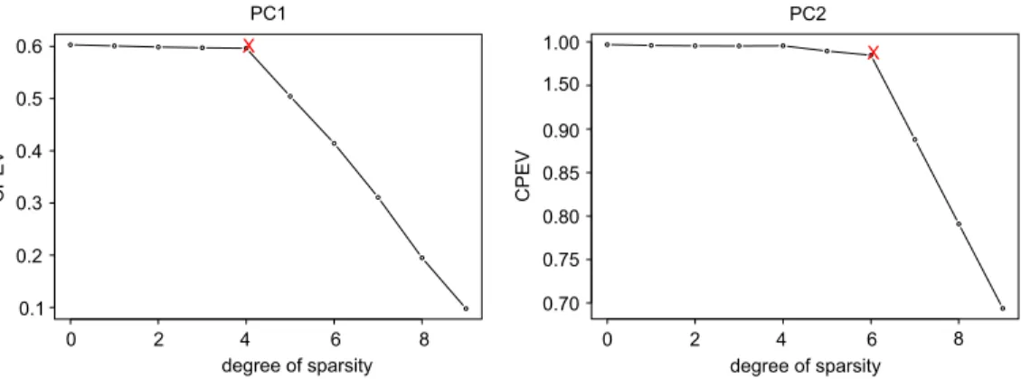
We now use the ad hoc approach (Section 2.5.2) along with sPCA-rSVD-hard to select the “optimal” degree of sparsity. Fig. 1 plots the CPEV as a function of the degree of sparsity for the first two PCs, which suggests that the degree of sparsity is 4 and 6, respectively, different from the suggestion of Zou et al. The two leading sparse PCs explain about 98.5% of the total variance, slightly less than the corresponding 99.7% obtained by the standard PCA. The extracted PC loadings are reported in Table 4. According to Fig. 1, it is perceivable to argue that the sparsity for PC2 is 4 as well, thus increasing the CPEV to 99.6%, almost the same as the standard PCA.
0.2 0.1 0.3 0.4 PC1 degree of sparsity CPEV X 8 6 4 2 0.70 0.75 0.80 0 0.85 0.90 PC2 degree of sparsity CPEV X 0.6 0.5 1.00 1.50 8 6 4 2 0
Fig. 1. (Example 3) Plot of CPEV as functions of sparsity. The degrees of sparsity of the two loadings are suggested to be 4 and 6, respectively.
4. sPCA-rSVD-soft vs. SPCA
This section provides some remarks on two sparse PCA methods: our sPCA-rSVD-soft and SPCA of Zou et al.[20]. Both approaches relate PCA to regression problems, and then employ a lasso (L1) penalty to produce sparsity, as well as some iterative algorithm for computation.
Despite these similarities, there are major differences between the two approaches. First of all, they solve different optimization problems. As we discussed in Section 2.3, to get the first loading vector, sPCA-rSVD solves
min
v {−2Xv + v
2+|
v|1},
while the same argument yields that SPCA solves min
v {−2X
TXv + Xv2+v2+1|v|
1}.
The objective functions of the two optimization problems are different.
The difference in computational algorithm is also significant. Operationally, SPCA solves the following optimization problem:
(A,B)=argmin A,B n i=1 xi −ABTxi2+ k j=1 j2+ k j=1 1,jj1 s.t. ATA=Ik×k,
whereA= [1, . . . ,k]andB= [1, . . . ,k]withkbeing the number of PCs to be extracted.
This problem can be solved by alternating optimization overAandB. For a fixedA, the optimal
Bis obtained by solving the followingelastic netproblem[19],
ˆ
j =argmin j
Yj∗−Xj2+j2+1,jj1,
whereYj∗=Xj. This problem can be solved using the LARS-EN algorithm. For a fixedB, the optimalAcan be obtained by minimizingni=1xi −ABTxi2 = X−XBAT2, subject to
Table 5
Computing time (in s) for Example 1 with 100 simulated data sets
sPCA-rSVD-soft sPCA-rSVD-hard sPCA-rSVD-SCAD SPCA (k=1) SPCA (k=2)
n=30 1.36 1.06 1.75 13.00 142.50
n=300 1.77 1.61 1.85 10.32 60.40
ATA=I
k×k. This is a Procrustes problem, and the solution is provided by considering the SVD, XTXB=UDVT, and settingA=UVT. Zou et al.[20] also developed the gene expression arrays SPCA algorithm to boost the computation forp?ndata.
The iterative algorithm in sPCA-rSVD-soft involves somewhat simpler building blocks, in-cluding simple linear regression and componentwise thresholding rules. This simplicity makes sPCA-rSVD-soft much easier to implement. The sPCA-rSVD-soft is also computationally less expensive since there is no need to perform an SVD in each iteration (Table 5). The sPCA-rSVD procedure treats bothn > pandp?ncases in a unified manner.
We now discuss some numerical comparison of SPCA and sPCA-rSVD-soft. Both procedures are applied to the simulated data sets in Examples 1 and 2. Since SPCA does not have an au-tomatic procedure for tuning parameter selection, we let the number of zero loadings equal to its true value for each loading vector. SPCA is implemented withk = 1 and 2, respectively, and generates different results (Tables 1 and 3). The sPCA-rSVD-soft does a better job than SPCA, especially the SPCA withk = 1. From boxplots of the estimated loadings (not shown here), we also observe that SPCA results in larger bias and variance when estimating the non-zero loadings. It is not well understood why the performance of SPCA appears to be sensitive to the choice ofk. The sPCA-rSVD-soft does not have this problem since the PCs are extracted sequentially.
To get some idea of the computing cost of various sparse PCA procedures, Table 5 reports the CPU time used in producing the results in Example 1. The sPCA-rSVD seems to be computa-tionally more efficient than SPCA. The fact that SPCA takes longer time to run forn=30 than
n=300 is due to more iterations needed for algorithm convergence.
5. sPCA-rSVD-hard vs. simple thresholding
Simple thresholding is an ad hoc approach that sets zero the loadings whose absolute val-ues below a certain threshold. Although frequently used in practice, simple thresholding can be potentially misleading in several aspects [2]. Our sPCA-rSVD-hard procedure also sets zero the loadings with small absolute values via the hard thresholding rule. In spite of its similarity to simple thresholding, sPCA-rSVD-hard works very well in simulated examples (Sections 3.2 and 3.3), and does not have the shortcomings of the simple thresholding discussed by Cadima and Jolliffe [2]. According to Table 1, while the performance of estimatingv1is comparable, sPCA-rSVD-hard improves over the simple thresholding forv2.
We think the difference is due to the way the thresholding is applied: sPCA-rSVD-hard applies hard thresholding on the loading vectors sequentially in an iterative manner; while simple thresh-olding extracts all the loadings first before applying hard threshthresh-olding. Therefore, the sparsity of the earlier PCs is not taken into account by simple thresholding when estimating the latter ones. Such a problem is avoided in rSVD-hard. Moreover, the sequential extraction allows sPCA-rSVD-hard to take into account the relationship between the variables, while simple thresholding fails to do so.
Table 6
(Example 3) Illustration of the instability of simple thresholding
Simple sPCA-rSVD-hard X1 0 0 0 0 0 0 X2 0 0 0 0 0 0 X3 0 0 0 0 0 0 X4 0 0 0 0 0 0 X5 0 0.494 0.491 0 0.499 0.5 X6 0.500 0 0 0 0.500 0.5 X7 0.499 0 0 0.499 0.500 0.5 X8 0 0.493 0.491 0.500 0.500 0.5 X9 0.500 0.506 0.508 0.500 0 0 X10 0.501 0.507 0.509 0.501 0 0
The first loading vector is extracted to have 6 zero components.
We now use Example 3 in Section3.4 to further understand the difference. In the course of following Zou et al.’s suggestion to extract the first loading vector with 6 zero components, one shortcoming of simple thresholding is identified: its instability as a result of high correla-tion among the original variables. As we change random seed and simulate a new data matrix, the selection changes dramatically amongX5–X10. These variables are highly correlated due to the high correlation between the underlying factors V2 andV3. Table 6 presents the load-ings for five simulated data sets, and one can see the instability of simple thresholding clearly. For example, for the first data set, simple thresholding leaves out X5 andX8while including
X9 andX10. The result is rather misleading because X5–X8 are essentially the same, which should appear together. On the other hand, sPCA-rSVD-hard always selects these four vari-ables, and the loadings remain very stable among the simulations. Table 6 also reports the av-erage loading vector produced by sPCA-rSVD-hard, which is the same as the one obtained by SPCA.
6. Real examples
6.1. Pitprops data
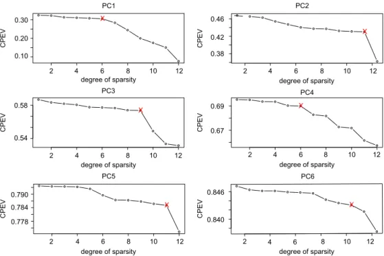
Jeffers [9] used the pitprops data to illustrate the difficulty of interpreting PCs, which have 180 observations and 13 variables. The correlation matrix of the pitprops data has been used repeatedly in the literature to illustrate various sparse PCA methods [12,20]. Following the literature, below we apply our sPCA-rSVD approaches to the pitprops data to extract thefirst sixsparse PC loading vectors.
Since the data matrix is a correlation matrix, we apply our procedure to its square-root matrix as justified by the discussion in Section 2.4. The ad hoc parameter selection procedure in Section 2.5.2 is used to select the tuning parameters. Below we present the result from sPCA-rSVD-soft. The CPEV selection plot is in Fig. 2, with thesubjectivelyselected degree of sparsity marked for each PC, which are 6, 11, 9, 6, 11 and 10, respectively. Table 7 reports the loading vectors by PCA and sparse PCA. The loadings from sPCA-rSVD-soft are much more sparse than the regular loadings, yet still account for nearly the same amount of variance (84.5% vs. 87.0%). See Zou et al. [20] for sparse PC loadings obtained by simple thresholding, SCoTLASS and SPCA.
12 10 8 6 4 2 2 4 6 8 10 12 12 10 8 6 4 2 PC1 degree of sparsity CPEV X 0.38 0.42 0.46 PC2 degree of sparsity CPEV X 2 4 6 8 10 12 0.54 0.790 0.784 0.778 PC3 degree of sparsity CPEV X 0.67 0.69 PC4 degree of sparsity CPEV X 2 4 6 8 10 12 2 4 6 8 10 12 PC5 degree of sparsity CPEV X 0.840 0.846 PC6 degree of sparsity CPEV X 0.30 0.20 0.10 0.58
Fig. 2. (Pitprops data) CPEV plot for sPCA-rSVD-soft with selected degrees of sparsity marked.
Table 7
(Pitprops data) Loadings of the first six PCs by PCA and sPCA-rSVD-soft
Variable PCA sPCA-rSVD-soft
PC1 PC2 PC3 PC4 PC5 PC6 PC1 PC2 PC3 PC4 PC5 PC6 x1 −0.404 0.218 −0.207 0.091 −0.083 0.120 −0.449 0 0 −0.114 0 0 x2 −0.406 0.186 −0.235 0.103 −0.113 0.163 −0.460 0 0 −0.102 0 0 x3 −0.124 0.541 0.141 −0.078 0.350 −0.276 0 −0.707 0 0 0 0 x4 −0.173 0.456 0.352 −0.055 0.356 −0.054 0 −0.707 0 0 0 0 x5 −0.057 −0.170 0.481 −0.049 0.176 0.626 0 0 0.550 0 0 −0.744 x6 −0.284 −0.014 0.475 0.063 −0.316 0.052 −0.199 0 0.546 −0.176 0 0 x7 −0.400 −0.190 0.253 0.065 −0.215 0.003 −0.399 0 0.366 0 0 0 x8 −0.294 −0.189 −0.243 −0.286 0.185 −0.055 −0.279 0 0 0.422 0 0 x9 −0.357 0.017 −0.208 −0.097 −0.106 0.034 −0.380 0 0 0 0 0 x10 −0.379 −0.248 −0.119 0.205 0.156 −0.173 −0.407 0 0 0.283 0.231 0 x11 0.011 0.205 −0.070 −0.804 −0.343 0.175 0 0 0 0 −0.973 0 x12 0.115 0.343 0.092 0.301 −0.600 −0.170 0 0 0 −0.785 0 0.161 x13 0.113 0.309 −0.326 0.303 0.080 0.626 0 0 −0.515 −0.265 0 −0.648 Sparsity 0 0 0 0 0 0 6 11 9 6 11 10 CPEV 32.5 50.7 65.2 73.7 80.7 87.0 30.6 45.0 59.0 70.0 78.5 84.5 The degrees of sparsity of PCs are selected according to Fig.2.
6.2. NCI60 cell line data
Microarray gene expression data are usually HDLSS data, where the expression levels of thousands of genes are measured simultaneously over a small number of samples. The problem of gene selection is of great interest to identify subsets of “intrinsic” or “disease” genes which are
2000 1005
1000 500
0
number of nonzero loadings
PEV PCA sPCA-rSVD-soft sPCA-rSVD-SCAD sPCA-rSVD-hard 0.22 0.18 0.14 0.1 0.06
Fig. 3. (NCI60 data) Plot of PEV as a function of number of non-zero loadings for the first PC.
biologically relevant to certain outcomes, such as cancer types, and to use the subsets for further studies, such as to classify cancer types. Several gene selection methods in the literature build upon PCA (or SVD), such asgene-shaving[8] andmeta-genes[18].
We use sparse PCA as a gene selection method and investigate the performance of various sparse PCA methods using the NCI60 cell line data, available athttp://discoer.nci.nih.gov/, where measurements were made using two platforms, cDNA and Affy. There are 60 common biological samples measured on each of the two platforms with 2267 common genes. Benito et al. [1] proposed to use DWD [15] as a systematic bias adjustment method to eliminate the platform effect of the NCI60 data. Thus, the processed data havep=2267 genes andn=120 samples. The first PC explains about 21% of the total variance.
We apply our sPCA-rSVD procedures on the processed data to extract the first sparse PC. Fig. 3 plots the percentage of explained variance (PEV) as a function of number of non-zero loadings. As one can see, the PEV curves for sPCA-rSVD-soft/SCAD are very similar, both of which are consistently below the curve for sPCA-rSVD-hard. This suggests that, using the same number of genes, the sparse PC from sPCA-rSVD-hard always explains more variance. According to the sPCA-rSVD-hard curve, using as few as 200 to 300 genes, the sparse PC can account for 17–18% of the total variance. Compared with the 21%, explained by the standard PC, the cost is affordable. Simple thresholding and SPCA are also applied to this data set, and their PEV curves are similar to the sPCA-rSVD-hard/soft curves, respectively. Note that such similarities may not hold in general as shown in previous sections.
7. Discussion
Zou et al. [20] remarked that a good sparse PCA method should (at least) possess the following properties: without any sparsity constraint, the method reduces to PCA; it is computationally efficient for both smallpand largepdata; it avoids misidentifying important variables. We have developed a new sparse PCA procedure based on regularized SVD that have all these properties. Moreover, our procedure is statistically more efficient than standard PCA if the data are actu-ally from a sparse PCA model (Tables 1 and 3). Our general framework allows using different
penalties. In addition to the soft/hard thresholding and SCAD penalties that we have consid-ered, one can apply the Bridge penalty[6] or the hybrid penalty that combines theL0 andL1 penalties [14].
When the soft thresholding penalty is used, our procedure has similarities to the SPCA of Zou et al. [20]. On the other hand, as we have shown in Section 4, the two approaches exhibit major differences. It appears that our sPCA-rSVD procedure is more efficient, both statistically and computationally. One attractive feature of the sPCA-rSVD procedure is its simplicity. It can be viewed as a simple modification—adding a thresholding step—of the alternating least squares algorithm for computing SVD. There is no need to apply the sophisticated LARS-EN algorithm and solve a Procrustes problem during each iteration.
When the hard thresholding penalty is used, our procedure has similarities to the often-used sim-ple thresholding approach. Our procedure can be roughly described as “iterative componentwise simple thresholding.” It shares the simplicity of the simple thresholding; furthermore, through iter-ation and sequential PC extraction, it avoids misidentificiter-ation of “underlying” important variables possibly masked by high correlation, a serious drawback of simple thresholding.
Appendix A.
Lemma A.1. Letv=v/vandV= [v;v⊥]be ap×porthogonal matrix.Then we have
X−uvT2F = XV−uvTV2F = [Xv;Xv⊥] − [uv;0]2F
= Xv−uv2+ Xv⊥2F = v2Xv/v2−u2+ Xv⊥2F.
Thus,for a fixedv,minimization of (2) reduces to minimization ofXv/v2−u2. On the other hand,we have thatminu:u=1−u is solved byu = /.In fact,−u2 = 2+1−2,u,sinceu =1.By the Cauchy–Schwarz inequality,,u,with equality
if and only ifu=c.Hence,u =1implies thatc=1/.Combining all these,we obtain LemmaA.1.
Theorem A.1. Let Hk =VkVkTVk−1VkT and denote the ith row ofXasxiT.The projection ofxi onto the linear space spanned by the first k sparse PCs isHkxi.It is easily seen that
trXTkXk = in=1Hkxi2andtr
XTX = ni=1xi2.SinceHkxiHk+1xixi,
the desired result follows.
Lemma A.2. Simple calculation yields
X−uvT2F =tr(XXT)−2vTXTu+ u2v2.
Thus,minimization of(2)is equivalent to minimization of
−2vTXTu+ u2v2+P(v). (6)
According to LemmaA.1,for a fixedv,the minimizer of(6)isu = Xv/Xv,which in turn suggests that minimizing(6)is equivalent to minimizing−2Xv + v2+P(v).
Theorem A.2. According to our procedure,v1is the minimizer of(6) andu1 =Xv1/Xv1.
LemmaA.2shows thatv1depends onXonly throughXTX.Our procedure derives the sparse
loading vectors sequentially.Form the residual matrixX1=X−u1vT1 =X
The second sparse loading vectorv2is the minimizer of(6)withXreplaced byX1.Thus,v2depends
onX1only throughXT1X1=
I−v1v1T/Xv1XTXI−v1vT1/Xv1,which implies thatv2
depends onXonly throughXTX.Moreover,
u2=X1v2/X1v2 =X
I−v1vT1/Xv1
v2/X1v2.
By induction,we can show that the residual matrixXk−1of the firstk−1PCs is
Xk−1=X k−1 i=1 I−vivTi /Xi−1vi ,
whereX0≡X.Furthermore,vkdepends onXonly throughXTX,and
uk =Xk−1vk/Xk−1vk =X k−1 i=1 I−vivTi /Xi−1vi vk/Xk−1vk.
As a result,v1, . . . ,vkdepend onXonly throughXTX.
Theorem A.3. LetVk = [v1, . . . ,vk]be the loading matrix of the first k loading vectors.Then,
as discussed in Section2.3,the corresponding projection isXk =XVkVT kVk −1 VT k ≡XHk. It follows that tr XTkXk =tr XkXkT =tr XHk2XT =tr XTXHk .
According to TheoremA.2,Hkdepends onXonly throughXTX,so doestrXT kXk
.
Acknowledgment
The authors want to extend grateful thanks to the Editors and the reviewers whose comments have greatly improved the scope and presentation of the paper. Haipeng Shen’s work is partially supported by National Science Foundation (NSF) grant DMS-0606577. Jianhua Z. Huang’s work is partially supported by NSF grant DMS-0606580 and a grant from NCI.
References
[1]M. Benito, J. Parker, Q. Du, J. Wu, D. Xiang, C.M. Perou, J.S. Marron, Adjustment of systematic microarray data biases, Bioinformatics 20 (2004) 105–114.
[2]J. Cadima, I.T. Jolliffe, Loadings and correlations in the interpretation of principal components, J. Appl. Statist. 22 (1995) 203–214.
[3]D. Donoho, I. Johnstone, Ideal spatial adaptation via wavelet shrinkage, Biometrika 81 (1994) 425–455.
[4]C. Eckart, G. Young, The approximation of one matrix by another of lower rank, Psychometrika 1 (1936) 211–218.
[5]J. Fan, R. Li, Variable selection via nonconcave penalized likelihood and its oracle properties, J. Amer. Statist. Assoc. 96 (2001) 1348–1360.
[6]I. Frank, J. Friedman, A statistical view of some chemometrics regression tools, Technometrics 35 (1993) 109–135.
[7]K.R. Gabriel, S. Zamir, Lower rank approximation of matrices by least squares with any choice of weights, Technometrics 21 (1979) 489–498.
[8]T. Hastie, R. Tibshirani, A. Eisen, R. Levy, L. Staudt, D. Chan, P. Brown, Gene shaving as a method for identifying distinct sets of genes with similar expression patterns, Genome Biology 1 (2000) 1–21.
[10]I.T. Jolliffe, Rotation of principal components: choice of normalization constraints, J. Appl. Statist. 22 (1995) 29–35.
[11]I.T. Jolliffe, Principal Component Analysis, second ed., Springer, New York, 2002.
[12]I.T. Jolliffe, N.T. Trendafilov, M. Uddin, A modified principal component technique based on the LASSO, J. Comput. Graph. Statist. 12 (2003) 531–547.
[13]I.T. Jolliffe, M. Uddin, The simplified component technique: an alternative to rotated principal components, J. Comput. Graph. Statist. 9 (2000) 689–710.
[14]Y. Liu, Y. Wu, Variable selection via a combination of theL0andL1penalties, J. Comput. Graph. Statist., 2007,
accepted for publication.
[15]J.S. Marron, M. Todd, J. Ahn, Distance weighted discrimination, J. Amer. Statist. Assoc. 2005, tentatively accepted for publication.
[16]R. Tibshirani, Regression shrinkage and selection via the lasso, J. Roy. Statist. Soc. Ser. B 58 (1996) 267–288.
[17]S. Vines, Simple principal components, Appl. Statist. 49 (2000) 441–451.
[18]M. West, Bayesian factor regression models in the “Large p, Small n” paradigm, Bayesian Statist. 7 (2003) 723–732.
[19]H. Zou, T. Hastie, Regularization and variable selection via the elastic net, J. Roy. Statist. Soc. Ser. B 67 (2005) 301–320.
[20]H. Zou, T. Hastie, R. Tibshirani, Sparse principal component analysis, J. Comput. Graph. Statist. 15 (2006) 265–286.