Fall 2019
Selection of regression estimators : simulation and application to
Selection of regression estimators : simulation and application to
the National Resources Inventory
the National Resources Inventory
Gani Agadilov
Follow this and additional works at: https://lib.dr.iastate.edu/creativecomponents Part of the Statistics and Probability Commons
Recommended Citation Recommended Citation
Agadilov, Gani, "Selection of regression estimators : simulation and application to the National Resources Inventory" (2019). Creative Components. 366.
https://lib.dr.iastate.edu/creativecomponents/366
This Creative Component is brought to you for free and open access by the Iowa State University Capstones, Theses and Dissertations at Iowa State University Digital Repository. It has been accepted for inclusion in Creative Components by an authorized administrator of Iowa State University Digital Repository. For more information, please contact [email protected].
Resources Inventory
by
Gani Agadilov
A Creative Component submitted to Department of Statistics in partial fulfillment of the requirements for the degree of
MASTER OF SCIENCE
Major: Master of Science in Statistics
Program of Study Committee: Dr. Emily Berg, Major Professor
Dr. Mark Kaiser Dr. Max Morris
Iowa State University Ames, Iowa
2019
TABLE OF CONTENTS
1 Introduction . . . 4
1.1 General information . . . 4
1.2 Literature review . . . 7
1.3 Overview of the application of methods . . . 11
2 Simulation study . . . 13
2.1 Simulation for covariate selection . . . 13
2.2 Simulation study with different g-distance functions . . . 17
3 Data analysis . . . 20
3.1 Overview of National Resourses Inventory dataset . . . 20
3.1.1 Specific NRI data sets used for the analysis . . . 21
3.1.2 Introduction to CDL auxiliary data source . . . 22
3.1.3 Varaince estimation for the NRI dataset using replicate weights 22 3.2 Evaluation of initial estimators and auxiliary information . . . 24
3.3 Subjective covariate selection approach . . . 26
3.4 Subjective covariate selection approaches with g-distance functions . . . 28
3.5 Automated covariate selection methods . . . 30
3.5.1 Selection of explanatory varaibles with stepAIC . . . 30
3.5.2 Selection of explanatory variables with LASSO . . . 31
3.6 Smoothing regression coefficients with RIDGE . . . 34
3.7 Using regression trees to group the CDL categories . . . 35
4 Discussion . . . 37
Preface
In spring 2019, I did an independent study in survey sampling. During the independent study, I expressed interest in regression estimation. In particular, I asked my supervisor if one could use the AIC criterion to select the covariates to use in the regression estimator. My supervisor suggested that I try my idea by conducting a simulation where I use the AIC criterion to select the covariates to use in the regression estimator. The interest that I expressed in regression estimation during my independent study partially motivated the topic of this creative component: regression estimation for surveys.
Regression estimation is a way to use auxiliary information to improve the efficiency of survey estimators. Regression estimation generates a weight such that the weighted sum of auxiliary variables for sampled elements is equal to known population totals. One can view the weight defining the regression estimator as the solution to an optimization problem. The regression weight minimizes the distance to the inverse inclusion probability subject to the calibration restriction. The calibration restriction forces the weighted sum of the auxiliary variable to equal the known population total.
We consider two issues arising in regression estimation. The first is the question of how to choose which covariates to include as control totals. The second is the choice of the metric defining the distance between the regression weights and the inverse inclusion probabilities. We explore these two issues through simulation and through an application to data from the National Resources Inventory.
The simulations are presented in Section 2. We first consider the use of the AIC criterion to select the covariates to use in regression estimation. The penalty defining the AIC criterion is developed under an assumption of simple random sampling. Lumley and Scott (2015) modify the penalty to appropriately reflect the effective sample size of a complex survey design. They use the modified AIC criterion to compare several models of interest for analytic inference. We consider a simplification of the Lumley and Scott (2015) modified AIC for the purpose of selecting auxiliary variables for regression estimation. Our modification to the AIC criterion is simple to implement using the stepAIC R function. In the second part of the simulation, we
consider the choice of the metric (the “g-function”). Different distance functions have connections to different log likelihoods. Specifically, “linear,” “raking,” and “logit” distance functions have connections to likelihoods of “normal,” “Poisson,” and “bernoulli” distributions, respectively. We therefore ask if certain distance functions lead to more efficient estimators than others for different response distributions.
In the data analysis of Section 3, we consider regression estimation for the National Re-sources Inventory (NRI). The NRI is a longitudinal survey that collects information related to land-use and agriculture. Satellite data offer the potential to improve efficiency with little additional data collection costs. A basic way to incorporate satellite data is through regression estimation. A simple satellite derived product is the Cropland Data Layer (CDL), a land-cover map based on automated classification of satellite images. We conduct a preliminary assess-ment of possible benefits from using the CDL to improve the efficiency of NRI estimators. We construct regression estimators using the NRI pointgen as our survey data and using the CDL as our auxiliary data. We use land-use data for Kansas from 2007 and 2012. We focus on corn, wheat, oats, cotton, and urban land-uses to obtain a variety of land-use categories. The CDL has approximately 30 categories for Kansas, and many of the categories have small NRI sample sizes. Therefore, reducing the dimension of the CDL covariate is necessary. We consider “selec-tion” and “grouping” as ways to reduce the dimension of the CDL. We define “selec“selec-tion” to refer to the process of removing certain CDL categories from the set of control totals. In contrast, we define “grouping” to refer to the process of combining small CDL categories into larger groups. We recognize that selection is a special case of grouping where all omitted categories are com-bined. Nonetheless, the distinction between selection and grouping will aid in our discussion. We compare four main ways to reduce the dimensionality of the CDL covariate: selection based on subjective analysis, grouping based on subjective analysis, automated selection using the AIC criterion, and automated grouping based on regression trees. We also compare regression estimators constructed with different distance functions in the data analysis.
We summarize our main conclusions in the discussion of Section 4. The modified AIC criterion provides a simple, automated way to obtain data-driven guidance on which covariates to use in the regression estimator. Nonetheless, in practice, we find that automated dimension
reduction procedures benefit from the aid of substantive knowledge. The data analysis offers insight into the possible benefits and limitations from using the CDL as an auxiliary data source in NRI estimation.
The results for the simulation study are presented. However, tables and graphs are removed from the data analysis section to protect the confidentiality of the data. The National Recources Inventory dataset has detailed information about agriculture sector of Kansas state that requires privacy. Therefore, the results for regression estimators and standard errors for particular type of crops and year are removed from the paper. Complete output is available from the authors.
1
Introduction
In a sample survey with complex sampling designs, auxiliary variables are often used to increase the precision of the estimation. One of the main objectives is how to effectively use the explanatory variables to receive an efficiency gain. As general information, we summarize concepts of the statistical theory of sample design and estimation in Section 1.1. Then, we review literature on regression estimator for survey in a Section 1.2. Finally (in Section 1.3), we overview the contents of this creative component.
1.1 General information
We consider regression estimation for sample surveys. First, we define the finite population framework and the regression estimator. Let U = {1, .., N} be the index set for the target
population. The variable of interest is yi for i= 1, .., N. We also observe covariates xi for
i= 1, .., N. Let a sample s ⊆ U be selected with first and second order inclusion probability
defined by πi and πij. The first and second order inclusion probabilities defined as follows:
1. First-order inclusion probability:
πi =P r(i∈s) =Ps:i∈sP r(s)
2. Second-order inclusion probability, or joint inclusion probability:
πij =P r(i, j∈s) =Ps:i,j∈sP r(s)
Inaddtion, inclsuion probabilities should hold following properties: 1. Probability sampling design: πi >0,∀i∈s
2. Measurable sampling design : πij >0i,∀j ∈s.
We are interested in estimating population means and totals for yi. The population mean
is defined as Y =N−1 N X i=1 yi. (1)
The population total is defined as
t=
N X
i=1
A standard unbiased estimator of the population total is the Horvitz-Thomson (HT) esti-mator. The HT estimator is defined as
ˆ tyπ = X i∈s yi πi . (3)
The general formula for the variance of the HT estimator is defined as ˆ V(tyπ) = N X i=1 N X j=1 (πij−πiπj) yi πi yj πj . (4)
The variance of the HT estimator for simple random sample is defined as
Vsrs(ˆtyπ) =N2(1− n N) Sy2 n (5) where Sy2= N−11 PN i=1(yi−Nt)
We can use the covariatexi to try to obtain an estimator that is more efficient than the HT
estimator. We will consider the regression estimator. The regression estimator is defined as ˆ tyreg = X s wiyi = ˆtyπ+ (tx−tˆxπ)Bˆ (6) wheretˆxπ =Psxπi
i denotes the HT estimator for the x-vector,and
ˆ B = (P s xix0i πi ) −1P s xiyi πi
We can rewrite the formula for the weight as
wi =π−1i + (tx−ˆtxπ)0(Psπ −1 i xix
0
i)−1xiπi−1.
and for the special case of simple random sample
wi = Nn + (tx−tˆxπ)0(Psxix0i)−1xi
The general formula for the estimated variance of the regression estimator is defined as ˆ V(ˆtyreg) = X i∈s X j∈s 4ij πij (wiei)(wjej) (7) where
4ij =πij −πiπj and eij =yi−(xi)0Bˆ.
The variance of the regression estimator for simple random sample is defined as
Vsrs(ˆtyreg) =N2(1− n N) Sy2 n (1−R 2) (8) where S2 y = N−11 PN
i=1(yi−y), R2 = 1−SSESST , and SSE and SST are residual error and
corrected total sum of squares from the population ordinary least squares regression ofyi onxi.
The weight of the regression estimator can also be defined through an optimization problem. The weightswi minimizes
P
s(wi−π −1 i )2
πi−1 , (9)
subject to the calibration constraint that P
swixi =tx.
The weightwi can be found using the method of Lagrange multiplier. In this approach,
wi =πi−1(1 +xiλ) (10) whereλ= (P s xix0i πi ) −1(t x−ˆtxπ)0.
This suggest a more general class of regression estimators. Deville and Sarndall (1992) define a general class of distance functions. The weight defining the generalized regression estimator minimizes P
sg(wi, πi−1) subject to the calibration restriction that Pswixi = tx.
Two common distance functions other than the squared error distance function are the raking and logit distance functions. The raking distance functions is defined
g(wi, π−1i ) =wilog(πw−i1
i
)−wi+π−1.
The raking distance function ensures that all of the weights are non-negative, while the linear function can lead to negative weights. However, the raking distance function may also lead to extremely large weights in some cases. The logit distance function enables the analyst to specify bounds. This distance function is identified as
g(wi, πi−1) = (x−L)log(x−L1−L) + (U −x)log(U−xU−1)
where L and U are two constants that specify the lower and upper boundaries of the weights, and x= wi
1.2 Literature review
A seminal work in regression estimation is Deville and Sarndal (1992). Since then many other works have dealt with the issues of choosing a metric (g-function) and choosing the covariates. We will discuss some of these works in this section. First, we summarize two recent review papers : Breidt and Opsomer (2017) and Qixuan et al. (2017). Breidt and Opsomer (2017) reviewed the model-assisted approach with the modern techniques by using the data from the complex survey. The new methods address the problems of statistical agencies conducting surveys, because of the cost of the survey and demand for the precise estimate at smaller scales needed to use known information about the target population in survey estimates. The author argues that their construction recipe from model-assisted estimation enables researchers to incorporate covariates and prediction methods from the wide range of sources. They provided an asymptotic framework that suggests inference tool. The basis is the difference estimator based on the population fit of the prediction method, making the important connection between design-based and the model-based components. Qixuan et al. (2017) reviewed approaches to possible inefficiency in estimation resulting from using survey weights in the analysis. The work mainly focused on modification of the basic design-based weight, which is the inverse of the units inclusion probability. The techniques such as weight trimming, weight modeling and incorporating weights via modeling for survey models were applied and numerical study was conducted to compare these methods. In addition, to support the numerical study the real dataset was used and general recommendations with limitations of the numerical study stated. Next, consider literature related to choosing the ”g-function.” One work that has connec-tions to the choice of the g-function is Kim and Park (2009). In that paper, they define the calibration weight as the product of the inverse selection probability and a function, g, that is nonlinear in a parameter, lambda. They define lambda to satisfy the calibration equation. They develop connections between this approach to constructing a calibration weight and the use of generalized regression estimation, discussed above.
Finally, consider literature related to choosing the covariates. The model-assisted survey regression estimation with the lasso is analyzed by Mcconville et al. (2017) to improve the
efficiency of the survey regression estimators of the finite population totals . The main idea of the lasso is to add a penalty to the optimization function. This facilitates the use of lasso for covariance selection. They developed model-assisted survey regression estimator using the lasso and extended it to the adaptive lasso. For the finite populations and probability designs, asymptotic properties of the lasso survey regression estimator are derived. To estimate finite population, lasso survey regression weights are developed with the model calibration and ridge regression regression approximation approach. Based on the simulation study results, lasso or adaptive lasso is recommended in the situation where survey regression needs to be calculated; however, survey weights are not necessary to receive the lasso regression estimators. The author mentioned that application of these methods in other surveys may be limited due to availability of the auxiliary variables.
Park and Yang (2008) investigated the ridge regression estimation for survey samples to demonstrate the difference among regression weights , ridge regression weights and raking ratio weights. The authors replaced some of the linear constraints with added components in the objective function and derived the coefficient matrix for the added components such that the defined ridge regression estimator has approximately the minimum model mean square error. The non-negative ridge regression weights were generated by using quadratic programming. To demonstrate the efficiency gain, the regression weights, ridge regression weights, quadratic programming weights and raking ratio weights were utilized for estimating the population per-centiles. Results from a simulation study indicated that the use of the ridge regression estimator with the optimal coefficient matrix for the important variables might be recommended for the large scale surveys with many covariates.
Chambers (1996) assigned a unique weight to each element of the sample when internal consistency of the survey estimates is important. If in addition external constrains on key variables are required, then case-weights are computed via generalized least squares, based on an assumption that there might be negative weights. The author proposed a modified method of linear regression based on case-weight that provides non-negative weights by using ridge procedure, and model misspecification robustness via the inclusion of a nonparametric regression bias correction factor.
Lumley and Scott (2015) develop principled survey analogues of AIC and BIC for fixed-effects regression models fitted using pseudo-likelihood methods. In this work, AIC is modified by inflating the penalty term by a design effect related to the Rao–Scott correction for log-linear models. In order to develop design-based analogues of AIC and BIC in other situations, similar approaches can be applied.
Toth and Eltinge (2012) proposed a method for incorporating information about the complex sample design when building a regression tree using a recursive partitioning algorithm. The authors’ work established sufficient conditions on the population distribution, survey design, and recursive partitioning algorithm that guarantee asymptotic design consistency of regression trees as an estimator for the conditional mean of the population. This investigation provided strong evidence that ignoring the complex design of the sample when using recursive partitioning approaches may have some negative consequences. The authors also offered a beginning to providing theoretical justification for using recursive partitioning algorithms on survey data.
McConville and Toth (2018) have presented the regression tree estimator for a finite pop-ulation total and have developed the design consistency of the estimator under standard as-sumptions on the sample design and finite population. The regression tree estimator is also a post-stratification estimator since a regression tree can be modified as a linear model where each variable is an indicator function for the sequential splits to an end node of the tree. There-fore, the regression tree can be viewed as a data-driven method to select the appropriate set of post-strata. These post-strata have the ability to capture complex interactions between the variables and they can increase the efficiency of the model-assisted estimator. Additionally, the estimator is calibrated to the population totals of each post-strata. They have focused on use-ful features of how regression trees handle categorical data, such as, collapsing categories into homogeneous subgroups and capturing predictive interactions between specific categories. The authors established consistency of the regression tree estimator and compare its performance to other survey estimators using the US Bureau of Labor Statistics Occupational Employment Statistics Survey.
The use of classification and regression tree has also been used to model survey nonresponse. Lohr et al.(2015) explored the effect of survey weights and clustering, pruning criteria, and loss
functions in an approach of regression trees to nonresponse modeling. The authors mainly focused on the effects of using sampling weights and differences among the algorithms. The machine learning methods to data analysis provides the many tools which can be utilized by survey researchers in a variety of context. Model-based recursive partitioning has been consid-ered as a data-driven tool for finding an optimal set of subgroups when the regression model is not correct. Klauch and Kreuter (2019) provided the usage of the application in the con-text of modeling and predicting nonresponse in panel surveys. The authors mainly focused on tree-based learning methods which enable to adapt to complex surveys and might be compu-tationally effective. They showed that tree-based ensemble methods is effective when studying nonresponce from a prediction perspective.
Bayesian methods have also been used to define weights modification. A Bayesian approach to defining survey weights is discussed in Si et al. (2017), which combine Bayesian prediction and weighted inference as a unified approach to survey inference. The authors constructed stable and calibrated model-based weights to solve the problems of classical weights. Model-based weights are smoothed across poststratication cells and improve small domain estimation. The hierarchical structure between main effects and high-order interaction terms are used for the structured prior to introduce multiplicative constraints on the corresponding scale parameters and informs variable selection. The authors stated that model can be improved can after post-processing the posterior inferences. The Bayesian structural model indicates more stable inference than that with independent prior distributions. Furthermore, the unified prediction and weighting approach is can handle common issues is surveys, such as complex designs and large number of variables.
Several of the procedures to select the covariates use modern techniques such as Bayesian models and regression trees. The textbook "The elements of statistical learning" discusses these procedures in general. In addition, generalized additive models, trees, multivariate adaptive regression splines, the patient rule induction method, and hierarchical mixtures of experts are introduced. We cite this textbook because we used it as a reference for an analysis using regression trees in Section 3.
1.3 Overview of the application of methods
The auxiliary information can be used to enhance of the precision of estimates of population total. In this work, we investigate calibration estimators proposed by Deville and Sarndal (1992). We consider a real data set from the National Resources Intentory(NRI). The NRI is a longitudinal survey of soil, water, and related environmental resources designed to assess conditions and trends on non-federal US lands. We also conducted simulation studies. We mainly focused on two different issues : choice of the different g-functions and choice of the appropriate covariates.
In Chapter 2, simulation studies consist of two parts. The first adresses the issue of covariate selection. We evaluate the use of AIC to select the covariates for regression estimation. Following Lumley and Scott (2015), we modify the AIC criterion to account for a cluster design. The second part of the simulation provides the evaluation of using different g- distance functions. As the g-function, three types of distance functions were chosen. There were linear, raking and logit. The regression estimator and variances were computed to demonstare efficiency.
In Chapter 3, in order to compare the impact of different auxiliary variables, different sets of explanatory variables were used in the regression estimator. The main crops such as corn and wheat were chosen to construct basic estimators. The subjective covariate selective approach was applied to identify the regression estimator. Then, different sets of covarietes were selected. Initially, corn and wheat were considered as more important crops in this region. Then, two CDL categories such as oats and corn were added. The main objective of this method is to define the difference between main and other crops in given region. The urban was added to identify the difference in regression estimators. The final set of auxiliary information includes all the explanatory variables in the dataset. The data analysis part also has the automated selection of CDL variables. The first approach is selecting the explanatory variables with stepAIC function. Then, selected covariates were used to calculate the regresion estimator. The different penalty parameters were applied. Another approach is selecting objective covariates by using least absolute shrinkage and selection operator (lasso). The set of auxiliary variables to remains the same. The three different g-fucntion were used to see the impact on regresion estimator. The
variance of lasso regression estimators with different distance functions provides the efficency gain for different sets of covariates. The ridge regression estimator was applied for the same set of covariates. Smoothing regression coefficients with ridge was compared with other regression estimators by difference in variances. The regression tree was used to select and group CDL categories for calculating the regresion estimators. The unordered and ordered CDL factors provided the objective grouping approach. We compare the impact of different set of covariets on the regression tree.
The disscussion section summarizes all methods and results of simulation and data analysis section. The future work for possible topics in given area are disscused.
2
Simulation study
2.1 Simulation for covariate selection
The main goal for this study is to provide the efficiency of selecting appropriate explanatory variables with different sampling designs. The simulation study is conducted by using the Monte Carlo method in order to indicate the gain of the different estimates of the population total. The notaion for generating model for simple random sample as following:
yi =β0+β1x1i+β2x2i+ei (11)
x1i∼ N(µ= 2, σ2= 0.5) x2i∼ N(µ= 3, σ2= 2.5)
x3i ∼ MN(p= (14,14,14,14,1) ei ∼ N(µ= 0, σ2e = 0.5)
For the simple random sample with one explanatory variable β0 = β1 = 1 and β2 = 0
(SRSx1) and for the simple random sample with two explanatory variables β0 = β1 = 1 and
β2 = 0 (SRSx1x2). The notaion for generating model for cluster sample as following:
yij =β0+β1x1ij+β2ijx2i+bi+eij (12)
x1ij ∼ N(µ= 2, σ2= 0.5) x2ij ∼ N(µ= 3, σ2= 2.5)
x3ij ∼ MN(p= (14,41,14,14,1) eij ∼ N(µ= 0, σe2= 0.5)bi ∼ N(µ= 0, σ2b = 0.5)
i= 1, ...,5000cluster and j= 1,2 elements within a cluster
The three random explanatory variables and error term are generated to have the response vari-able. The two random variables are continious and one categorical variable with four categories. All continious random variables and error term are from a normal model with different mean and standard deviation parameters.
In the correct model, the single explanatory variable is used to compare the mean square error and standard error estimation between regression estimator and alternative regression estimators. In addition to the correct model with one explanatory variable, the model uses two explanatory variables to capture the gain with selecting the more correct variables. For the convenience, the population(10 000) and sample size (100) were equal in both sampling
methods, the sample seed was the same. The size of cluster for population and sample are (5000) and (50) respectively.
The mean square error, standard error, and efficiency of sampling techniques are calculated for four types of estimators. The first estimator is a basic estimator as Horvitz-Thomson (HT). The second estimator is a regression estimator (RE) that using the true model. The third and last estimators are alternative regression estimators with different penalty terms. The covariates are selected using Akaike information criterion (AIC). The regression estimator with AIC1 is standard case of AIC where penalty term is k= 2. The AIC2 case is simplification of Lumley.
The parameterk is computed by following formula and it is 2.6 which rounded to 3:
k= 2∗δ andδ = β21σ2x 100 + σ2b 50 σ2e 100 100 σx2+σ2 b+σe2 100
The denominator in the equation based on the mean for the clustered population would be
E[Sy2/n], where Sy2 = (2M −1)−1PMi=1P2j=1(yij −y¯..)2. We write E[(2M−1)Sy2]as E[(2M−1)Sy2] =E[ 2 X i=1 2 X j=1 (yij−y¯i.)2+ 2 M X i=1 (¯yi.−y¯..)2], (cross-term is zero) =E[ M X i=1 2 X j=1 ((xij −x¯i.)0β+ (eij−¯ei.))2+ 2 M X i=1 (¯x0i.β+bi+ ¯ei.)2] = M X i=1 [β0Σxxβ+σ2e] + 2(M −1)[β0Σxxβ/2 +σb2+σe2/2] = (2M −1)β0Σxxβ+ (2M −1)σe2+ (2M−2)σ2b.
The denominator would then be
E[Sy2/n] =β0Σxxβ/n+σe2/n+ (2M−2)/(2M −1)σb2/n. (13)
For large M, the denominator in (13) is nearly the same as the denominator that we used
because(2M−2)/(2M−1)≈1.
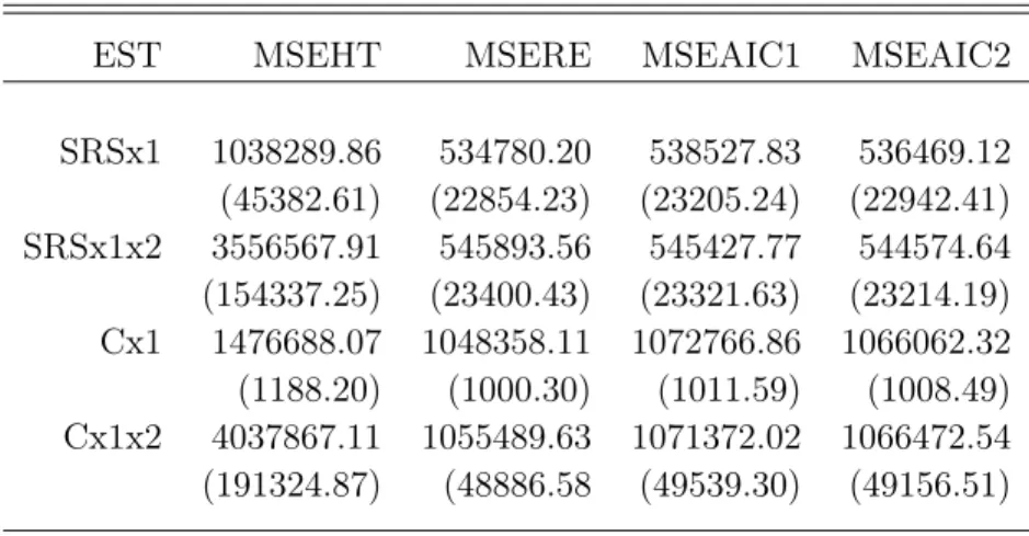
The Monte Carlo MSE is calculated for each method and sample design. The parentheses contain standard error for the MC approximating to the MSE’s (See Appendix3).
EST MSEHT MSERE MSEAIC1 MSEAIC2 SRSx1 1038289.86 534780.20 538527.83 536469.12 (45382.61) (22854.23) (23205.24) (22942.41) SRSx1x2 3556567.91 545893.56 545427.77 544574.64 (154337.25) (23400.43) (23321.63) (23214.19) Cx1 1476688.07 1048358.11 1072766.86 1066062.32 (1188.20) (1000.30) (1011.59) (1008.49) Cx1x2 4037867.11 1055489.63 1071372.02 1066472.54 (191324.87) (48886.58 (49539.30) (49156.51)
Table 1 Monte Carlo mean square error (standard error) for different estimators
Table 1 contains the comparison of Monte Carlo mean square error of the different type of estimators. As we expected, regression estimator is more efficient than HT in all cases. For SRSx1, using AIC to select the covariates (AIC1) leads to a significant increase in MSE relative to using the regression estimator based on the true model. The t-test statistic for RE and AIC1 is 2.7 and we reject the null hypothesis of no difference for SRSx1. It means that the estimators are statistically significant. For SRSx2, it is surprising that RE has larger MC MSEs than other estimates. The t-test for AIC1 and AIC2 provides the test statistic 1.9 for SRS x2 wchich is not statistically different. The simple random sample with two explanatory varables for RE and AIC1 cases have almost same results. By applying the t-test, we receive that test statistic is 0.38. It means the estimators are not statistically different.
Next, consider cluster sampling. The applied design have the expected results that using the true model leads to more effiicient estimates than using AIC to select the covariates. The t-test-statistic for RE and AIC2 is 4183.152 for Cx1. It indicates that estimators are statistically different. For this method, AIC2 is more efficient than AIC1 since AIC1 is selecting "too many" covariates. This illustrates how the MSE of the estimator can be adversely affecting. In other words, we have too many covariates in our model. The t-test for AIC1 and AIC2 are apllied and test statistic is 6840.316. This suggests that differences are statistically significant. The estimation pattern for the case with two expalantory variables is the same.
Effficency Simple and Cluster HT -5.54 Simple and Cluster REGEST -9.70 Simple and Cluster REGAIC1 -9.78 Simple and Cluster REGAIC2 -9.79
Table 2 Efficiency of sampling methods
simple random sample design to the cluster method. The two designs are comparable because our choices of sample size and varainces of error terms. We expected that simple random sample to be more effificent than cluster sampling. The results confirm that this is true case. Table 2
indicates that the simple random sample with one explanatory variable in the correct model more efficient than cluster sample. The result shows that simple random sample design for Horvitz-Thomson estimator is better than cluster sampling for the same estimator. However, the efficiency is almost the same when the alternative regression estimators with different penalty terms with two explanatory variables in the correct model.
2.2 Simulation study with different g-distance functions
The objective for the study is to provide the efficiency gain with different distance functions. The motivation for the study comes from connections between of the g-fucntions and different log likelihoods. The results of Kim and Park (2009) imply that the calibration estimator based on the raking distance function is asymptotically equivalent to the linear estimator defined as
ˆ Ty,` = X i∈s π−1i yi+ (Tx− X i∈s π−1i xi)0Bˆy|x,g, (14) where ˆ By|x,g = X i∈s xiexp(λ0xi)x0i !−1 X i∈s π−1i xiexp(λ0xi)yi,
andλ= 0. This means that the raking distance function and the linear distance function lead to
estimators with the same large sample distribution. Regardless, the form ofBˆy|x,g is related to
a Poisson log likelihood. AssumeYi∼Poisson(λi), whereλi=exp(x0iβ). Then the population
likelihood equations for estimating βare
X
i∈U
(Yi−exp(x0iβ))xi= 0.
This suggests that the raking distance function may be relatively well suited to a Poisson response random variable.
We conduct a simulation study to assess this. We generate xi ∼ N(0,0.25) for i =
1, . . . ,2000and generateYi ∼Poisson(λi), whereλi =exp(2 +xi). We select a simple random
sample of sizen= 50. We compute calibration estimators of the total ofY using the linear and
raking distance functions. We use a MC sample size of 50000. The MC MSEs of the estimators of the population totals based on the linear and raking distance functions are 857065.5 and 859853.1, respectively. The MSE of the estimator of the total based on the raking distance function is 2787 units smaller than the MSE of the estimator based on the linear distance function. The standard error of the MC estimator of the difference in MSE is 649 units. The difference in MSE is small but statistically significant.
This small but significant difference provides motivation for larger simulation study with 3 different distance functions. In order to indicate the difference in regression estimators the
Monte Carlo method approach was apllied. The three distance functions were selected: linear, raking, and logit. The logit distance function reguires the lower and upper limits. The weights from the dataset used for Section 3 is range between 0 and 258, therefore, the 0 and 260 bounds were chosen respectively. To generate response with Bernoulli distribution following notation is used:
yi =Bernoulli(pi, n), logit(pi) =β0+β1x1i (15)
x1i∼ N(µ= 2, σ2= 0.5)
The response variable for Poisson distribution uses the same explanatory varaible as in Bernoulli case and defined as following:
yi∼P oisson(λi), logit(λi) =β0+β1x1i (16)
Normal distribution is also used to generate response with same covarite and error term:
yi =β0+β1x1i+ei ei∼ N(µ= 0, σ2e = 0.5) (17)
The coefficients for all types of distributions are β0 = β1 = 1. The single explanatory
variable is used to compare the mean square error, standard error with simple random sample sampling. For the computaional convenience, population and sample sizes are 10 000 and 100 respectively.
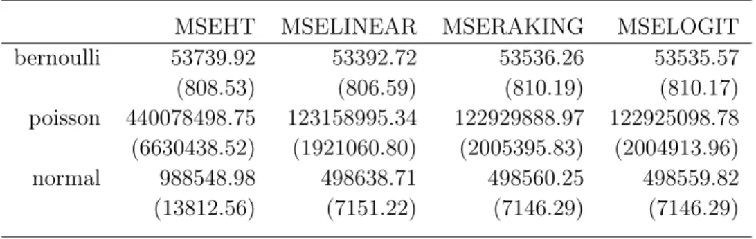
The mean square error and corresponding standard error are calculated the Horvitz-Thomson estimator, regression and further estimators constructed with different g-functions.
MSEHT MSELINEAR MSERAKING MSELOGIT
bernoulli 53739.92 53392.72 53536.26 53535.57 (808.53) (806.59) (810.19) (810.17) poisson 440078498.75 123158995.34 122929888.97 122925098.78 (6630438.52) (1921060.80) (2005395.83) (2004913.96) normal 988548.98 498638.71 498560.25 498559.82 (13812.56) (7151.22) (7146.29) (7146.29)
Table 3 contains the comparison of Monte Carlo mean square error of the estimators of the simple random sample with different distance functions. Firstly, we focused on bernoulli case. The table indicates that the mean square error with linear distance function are less than other estimators with raking and logit functions for bernoilli case. Regression estimators with different distance functions provide similar results. It needs to be checked that some estimators for statistically sifnificant. For instance, regression estimator with linear and raking distance functions compared for significance. The paired test approach is utilized. The t-test statistic is 7.737 and estimators are statistically different. The regression estimator with raking and logit function do not indicate much difference. However, the test statistic for that pair is 7.97 that shows that they are statistically different. The response variable with Poisson distribution provides unusual large estimates compared to other types of distributions. The regression estimator with linear and raking are compared and test statitic is 0.69. It suggest that two estimator are not statistically different. If we compare estimates with raking and logit distance functions, test statistic is 3.58. The p-value suggests that estimates are statistically significantly different. Surprisingly, normal distribution has smallest estimates for logit distance functions. The paired t-test is applied to compare estimates of raking and logit cases. The test statistic is 0.28 and regression estimators are not statistically significant. In addition, the test for significance is used to indicate difference for linear and logit distance functions. The test statistic is 0.62 which does not provides an evidence for statistical difference.
In summary, in these simulations, we see a negligible difference between distance functions. Part of the reason that the difference in MSE is small is that λ = 0 in Equation 14. If we
had non-response λ6= 0, and we may expect a greater difference between the linear and raking
distance functions. The question of finding model based motivation for using a particular distance function may be an area for future work. However, the main conclusion from this analysis is that the choice of the distance function is of little consequence.
3
Data analysis
3.1 Overview of National Resourses Inventory dataset
In data analysis section, we utilized the National Resourses Inventory (NRI) dataset from Kansas state. Kansas has been used as a test stage for NRI estimation because it is highly agriculture but more diverse with respect to agriculture production than Iowa. We investigated the choice of the covariate and the choice of the g-function using the NRI data.
The NRI is a longitudinal survey designed to assess natural resource conditions on non-federal lands in the United States. Center for Survey Statistics and Methodology at Iowa State University conducted many natural resource assessment surveys with the US Department of Agriculture’s Natural Resources Conservation Service.
The process of collecting and procedure of conducting an anlysis with NRI dataset have been developed on wide range of economical and political research questions. As we expected in Nusser and Goebel (1997), "The NRI is a national multi-resource inventory and monitor-ing programme whose purpose is to produce a longitudinal data base containmonitor-ing numerous agro-environmental variables that will support scientific investigations. Most of NRI’s specific objectives have been related to agriculture and natural resource conservation. These resources tend to exhibit moderately slow rates of change, although rapid alterations in land use, resource conditions, and practices may occur in response to discrete shifts in environmental conditions." Nusser and Goebel (1997) described statistical procedures used during the 1992 survey, includ-ing sample selection, data collection, imputation of missinclud-ing data, and weight calculation.
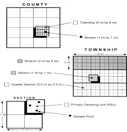
The original NRI sample was selected using a stratified two-stage design. "The choice of design for any survey depends on the objectives of the survey, the nature of the population, and operational constraints", as explained in Nusser and Goebel (1997). The land area of the majority of states in the US is divided according to the Public Land Survey system, illustrated in Figure1. The PLS system divides townships into 36 square sections, each one mile on a side. NRI strata are groups of 12 sections. A typical PSU is a 160-acre square quarter-section, 0.5 miles on each side. Three sample points are selected within each PSU.
Figure 1 Graphical representation of NRI primary sampling unit and sample points
NRI estimation involves weight construction, imputation of missing values, and adjustments to meet desired control totals. The initial weight is the inverse inclusion probability multiplied by the segment acres divided by the number of points per segment. Federal and large water areas (estuary and waterbody larger 40 acres ) are obtained from administrative sources. The final NRI estimation database is called the "pointgen". Each record in the pointgen has a single weight and a complete time series of NRI varaibles of intereset.
3.1.1 Specific NRI data sets used for the analysis
The NRI dataset for the data analysis section is taken from Kansas state in 2007 and 2012. The number of categories in dataset in NRI land uses and CDL land uses are 33 and 29 respectively. Before conducting the analysis, the federal and large water categories are removed from the dataset since these categories are known from administrative sources. In addiotion, we use final 2012 NRI estimation data set. While the estimator is more complex then the HT estimator, the final NRI estimator will be the initial survey estimator for our analysis. We call
the initial survey estimator the HT estimator. We will try to improve initial estimator using additional auxiliary information that is not already used in NRI estimation.
3.1.2 Introduction to CDL auxiliary data source
Cropland Data Layer (CDL) is a satellite data that uses to classify land cover use. Coter-minous U.S. divided into a 30x30 meter grid. In this area, every 30x30 cell is assigned a CDL land cover/use. While a NRI dataset uses a visual inspection, CDL utilize the algoritm to land cover classification.
3.1.3 Varaince estimation for the NRI dataset using replicate weights
We evaluate the varaince of regression estimators for NRI land cover/use using CDL as the covariate. In order to specify, the following notaion is used :
t = 07,12 year,k1 = 33NRI land uses and k2 = 29CDL land uses
yit = (yi1t, ..., yik1t) ;yikt=I[NRI point i is in LUk for yeart]
xit= (xi1t, ..., xik2t) ;xikt=I[CDL point i is in LUk for yeart]
wi - estimation weight for pointi
wir : r = 1,...,29 replicate weights for points ifor varaince estimation
The population is all area in Kansas. The inputs to regression estimator identifed as follow-ing: Population total and Horvitz-Thomson estimator for x :
tx,t= X U xi,t ˆtxπ,t= X s wixit. (18)
Initial NRI estimator for y:
ˆ
tyπ,t= X
i∈s
wiyit. (19)
Regression estimator, written as a function of the weights w={wi :i∈s}
ˆ
whereBˆy|x = (Pi∈swixixTi )−1 P
i∈swixiyi
The formula for the variance of HT estimator idendified as following: ˆ V(ˆtyπ,t) = 29 X r=1 (ˆt(r)yt −ˆtyπ,t)(ˆt(r)yt −ˆtyπ,t)T (21) whereˆt(r)yt =P i∈sw (r) i yit.
The formula for the variance of regression estimator described as following: ˆ
V(ˆtyreg,t) = 29 X
r=1
(ˆt(r)yreg,t−ˆtyreg,t)(ˆt(r)yreg,t−tˆyreg,t)T (22)
where tˆ(r)yreg,t = ˆtyreg,t(w(r)) wr= n
3.2 Evaluation of initial estimators and auxiliary information
In this section, we calculate basic estimators as a baseline for comparison. We first consider the NRI estimator from the 2012 NRI. We use the NRI estimator as the starting point from which we attempt to make improvements. The NRI estimator is more complex than the HT estimator because the weight defining the NRi estimator is not simply the inclusion probability. We refer to the NRI estimator as the HT estimator since we use it as the starting point for our analysis.
Design-weighted HT estimator and other regression estimators are calculated for five types crops in 2007 and 2012. In order to select the type of crops that objectively represent the given region, overall diversity of crops and the amount of acre age are taken into account. The main crops, corn and wheat have a large amount of acre age. In addition, datatset from 2007 and 2012 indicates that increasing trend of corn and decreasing trend for wheat. Therefore, we assumed that using these two type of crops to compare fundamental estimates to other regression estimators might be worthwile. Moreover, the other two types of crops that represent less acreage oats and cotton. We decided to identify the difference between estimators from crops that have large acre age with small acre age. Finally, the urban factor is included in the estimator. The main aim to include the last factor is because the issue of urbanization has been a topic of interest in the NRI.
Table 4 has the design-weighted HT estimator for corn, wheat, oats, cotton, urban in 2007 and 2012. It can be seen that estimaton for corn, oats, cotton and urban are increased whereas wheat has smaller estimator. It should be noted that some estimators shows slight increasing pattern, but HT estimator for cotton increased more than twice. Also table shows standard errors for the estimates of the change from 2007 to 2012. The ratio of the estimated change to the standard error of the estimator of the change exceeds 2 in absolute value for all LU’s except for oats.
We consider use Cropland Data Layer (CDL) as a covariate in regresssion estimation. The CDL is a land cover map based on satellite data. Table 5 shows the CDL categories for Kansas, and Table 6 shows the number of NRI points in each CDL category.
From Table 5, we can see that many of the CDL categories have small sample sizes. Some-times reseachers want to include all availabe explanatory varaibles and compare the output with subjective selection methods. This actually suggesting including all CDL varaibles. We cannot include all CDL factors since some CDL categories only have one NRI point. An attempt to control to CDL categories with only one NRI point results in an undefined variance estimator. Table 6 shows the number NRI points in Kansas in CDL category. To avoid small counts, we eliminated category fewer than 100 NRI points. We compute four ways to reduce the dimensionality of the CDL covariate in the next four sections.
3.3 Subjective covariate selection approach
First, we select covariates using subjective analysis. We consider two set of CDL categories for each year. We only use only the major crops corn and wheat. Second, we consider the 14 CDL categories with at least 100 NRI points. These 14 categories are assosicated "X" in Table 5. We also construct regression estimator using 14 CDL categories from both years. Table 7 contains the regression esimators, and Table 8 contains the corresponding standard errors. For the rows labeled "CDL YYYY", the covariates are corn and wheat for year "YYYY". For the rows labeled "ALL", the covarites are the 14 CDL categoires for the year intended in the row label name. One of the objectives of this first analysis is to examine the effect of including yearly CDL varaibles. Therefore, we consider including covariates for 2007 and 2012 separately. If we only include covariates for one year, then all distance functions yield the same estimator (See Appendix 1). Therfore, we only consider the linear distance function in this section.
Table 7 shows that corn and wheat factors from each year has different effect on regression estimators. For example, it can be seen that the regression estimator for corn in 2007 and 2012 is less than HT estimator for both years. This is expected because acre age in 2007 in Table 5 is smaller than HT07 for corn. Similarly, the HT estimator for urban is greater than the regression estimator for urban. The difference between the HT estimate and regression estimator is typically smaller than an estimated standard error. The difference is not significant, wich is reassuring, as we expect the NRI estimator to be design consistent. Therefore, we focus on in estimated varainces.
Table 8 shows the estimated standard error for each time point. If we include only 2007 for corn and wheat, it decreases the estimators variences for 2007. The 2012 variance for corn is also reduced but not as much as the 2007 estimate. The estimator of variance for wheat for 2012 actually increases when we iclude 2007 CDL variables as covariates. Conversely, including 2012 CDL varaibles leads to greater reducing in standard error for 2012 than for 2007. If we add only corn and wheat factor, it increases slightly the standard error for urban, oats and cotton covaraites.
essen-tially no change in the estimation in variance for cotton. The increase in the varaibility of the weights actually leads to an increase in the estimated standard error for oats for 2007. The results from all CDL factors in 2012 shows that estimators for corn and wheat had opposite pattern in comparison with estimates when we use all CDL factors in 2007. The estimated varinace for corn and wheat in 2012 is less than estimated varince for corn and wheat in 2007. The CDL factors from 2012 has a quite same impact on cotton, oats and urban as CDL factors from 2007. The variance estimator for urban factor in 2012 is quite less than 2007 estimates for urban variable. The analysis with CDL varainces for individual year shows that using yearly CDL variables is important. Therefore, we also select all 14 explanatory variables from 2007 and 2012 : the overall 28 factors selected from both year that have more than 100 NRI points. From the results, we can notice that variance of the regression estimators are more efficient for the corn, wheat and urban factors in both years. This inidcates that including too few CDL varaibles as covariates fails improve the efficiency for important variables.
Table 9 shows the estimators of change and corresponding standard errors for the 5 differ-ent types of regression estimators. In general, the improvemdiffer-ent in efficiency from using the regression estimator instead of the HT estimator is less important for the change than for level. In this section, we considered CDL categories with at least 100 NRI points. This as arbitrary cut-off value, but it seems to work relatively well. In the next section, we consider aggregating small CDL categories together. We have omitted CDL varaibles for oats and cotton, and the results show little change in the NRI estimators for large crop categories. In the next section, we consider including CDL categories for oats and cotton.
3.4 Subjective covariate selection approaches with g-distance functions
In the previous section we compare the results from regression estimators with two covariates and 14 covariates from different years. The results indicated that including all covariates from both years has an efficient effect on variance of regression estimators. In order to find an appropraite set of covariates, we paid an attention to the diversity of the crops and number of NRI points in the given area. We included corn and wheat factors from both years since they are major crops and have sufficient NRI points. Then, we decided to compare the impact on small crops. Therefore, the oats and cotton from 2007 and 2012 included to compute the regression estimator. The other factor as urban included in the estimation since this factor might indicate some important aspect of urabanization and potential arisining questions from agriculture sector. In addition, we decided use all available factors from the NRI dataset. In order to avoid from small NRI points, the same crop types combined to one main crop and considered as one CDL category. Thefore, we have used 14 CDL factors from both years and compared the regression estimators with linear,raking and logit distunce functions.
Table 11 below shows results from using different distance functions for different set of covariates. The 2 CDL means corn and wheat from both years, 4 CDL indicates that estimator has four type of crops which are corn, wheat, oats, and cotton. Then, 5 CDL means estimation includes a urban factor. The last set of covariates includes 14 CDL varaibles from 2007 and 2012 from NRI dataset. The table indictates that regression estimator by using 14 CDL factors for corn 2007 is less than other estimators. For the corn in 2012 the regression estimater with 2 CDL and 4 CDL provides smaller estimates. The wheat factor has smallest estimator with 14 CDL factors despite the type of the distance functions. The oats and cotton categories in 2007 has quite same estimates for different distance fucntions. However, the oats in 2012 has the smallest estimator for 2CDL for all tree types of distance functions. In contrast, cotton in 2012 has the largest estimate for 2 CDL factor. The urban factor for 2007 and 2012 has same pattern. The smallest estimates provides for 2CDL factor despite the distance functions, and largest for 14 CDL factor.
the output, it can be noticed that using the 14 CDL factors is more efficient than including other set of covariates in the estimation. The variance of regression estimators for corn in 2007, wheat in 2012 and urban in both years have linear varaince estimates. For crops as cotton and oats from both years variance of regression estimators have quite similar pattern. In addition, it should be noted that including the urban factor provides more efficient estimator, but not as much as with 14 CDL categories. Implementing estimation procedure with urban factor also decrease the variance for corn in 2012 and oats in 2007.
Table 13 and Table 14 shows that using the different distance functions does not change much. The varaince of regerssion estimator by using raking and logit distance functions have quite similar estimates. The results indicates that using all CDL categories assures more effi-ciency.
Table 15 indicates the variance of the difference between regression estimators for 2007 and 2012 with difference distance functions. As we see from the previous table results, the variance estimation for the corn and oats is less for 14 CDL factors. However, for wheat factor 4CDL categories is efficient. The cotton and urban factor has similar estimators. In summary, we can notice that the different distance function are all similar. The graphs for covariates in Table 10 are subjective. The next section explores other options to select objective set of covariates utilizing lasso, ridge and regression tree approaches.
3.5 Automated covariate selection methods
3.5.1 Selection of explanatory varaibles with stepAIC
In the previous sections, we reduced the dimensionality of the CDL categories using sub-jective methods. First, we selected CDL categories with at least 100 NRI points. Then, we grouped small CDL categories together. The criteria for selection and grouping were subjective. In this section, we consider automoted selection procedures. We first consider AIC. We consider two different values for the penalty parameter. The standard AIC penalty parameter is k= 2. The value of k= 2 is motivated from a simple random sample. The NRI is a cluster
sample with 3 points per cluster. We consider a different value fork to account for the cluster
design.
An estimated design effect for the NRI survey is defined as ˆ def f = ˆ VN RI(ˆpwheat07) ˆ pwheat07(1−pˆwheat07)/n , (23)
where pˆwheat07 is the NRI estimate of the proportion of area in Kansas in wheat in 2007, and
nis the total number of NRI points in the data set for Kansas. We obtain an estimated design
effect of 1.48. This provides justfifcation for our value ofk= 2(1.48)≈3. A”X”symbol in the table means that the corresponding covariate was selected. For example, AIC criteria selected corn in 2012, but not in 2007.
As a first step, we include an indicator varaible for each of the 29 CDL categories. We use the AIC criterion to select which CDL factors to include as covariates. We define 29 indicator variables to represent the 29 CDL categories. We use wheat in 2007 as a response variable and the 29 indicator varaibles as possible covariates. Althouhg wheat in 2007 is binary, we use squared error loss as the objective function for AIC. We use the stepAIC function in R to decide which CDL variables to include as covaraites. We usek = 2and k = 3 . With either value of
k, the stepAIC procedure includes Canola as apossible covariate. Canola a only has 1 sampled
point, which makes the varaince estimator undefined. Therefore, we will need to incorporate some subjective knowledge when implementing AIC.
We implemented stepAIC with two different sets of possible covariates and two different penalty parameters. Each row of Table 16 corresponds to a possible covariate to include in
the model. We consider including only 2007 covariates, only 2012 covaraites, and covariates for both 2007 and 2012. We begin with the 14 groups of CDL categories defined in Section 3.4, and the ask the question, "Can we reduce the dimentiality further using stepAIC?"
Then, we calculate regression estimators and corresponding standard errors using the covari-ates in Table 16. Table 17 contains the estimator and Table 18 contains the estimated standard errors. We only consider the linear distance function for this analysis. Table 18 indicates that the standard error for k=3 with CDL factors from both years leads to estimators that are more efficient than the other set of covariates. It can be noticed that standard errors for all factors have sufficient efficincy.
Table 19 shows the standard errors for regression estimators of change. As we can see that estimation with k= 2 has almost same result with penalty parameter k= 3.
3.5.2 Selection of explanatory variables with LASSO
The most known model selection approaches are best subset selection and stepwise selection. When the number of covariates is large the best subset selection is not easy to implement since the computation takes an immense amount of time. The stepwise selection needs less time and provides best model only locally.
"The "least absolute shrinkage and selection operator"(lasso) method proposed by Tib-shirani (1996) simultaneously performs model selection and coeffcient estimation by shrinking coefficients to zero. The lasso methods finds coefficients that minimize the sum of the squared residuals subject to a constraint on the sum of the absolute value of the coefficients. The coefficient estimates for lasso are given by:"
ˆ β = argmin β (Y −Xβ)T(Y −Xβ) +λX s |βj | (24)
where the estimate of the intercept β0 is not penalized and λ≥0. In order to use the LASSO
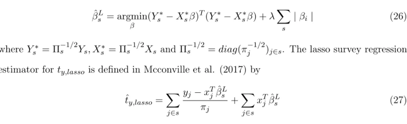
for a complex survey the survey-weighted lasso coefficient estimates are used. ˆ βLs = argmin β (Ys−Xsβ)TΠ−1s (Ys−Xsβ) +λ X s |βi|, (25)
where λ ≥ 0. The survey-weighted lasso coefficient estimates can be computed using the following equiation: ˆ βLs = argmin β (Ys∗−Xs∗β)T(Ys∗−Xs∗β) +λX s |βi | (26) whereYs∗ = Π−1/2s Ys, Xs∗ = Π −1/2 s Xs andΠ −1/2 s =diag(π −1/2
j )j∈s. The lasso survey regression
estimator forty,lasso is defined in Mcconville et al. (2017) by
ˆ ty,lasso = X j∈s yj−xTjβˆsL πj +X j∈s xTjβˆsL (27)
The lasso estimator does not provide a linear estimator. Therefore, we can not write a lasso survey regression estimator as a linear combination of the y values in the sample. Mcconville et al. (2017) defined a lasso calibration estimator is by regressing the study variable, yj, on
an intercept and the lasso-fitted mean fucntion, xTjβˆsL, over the sample. Then, xj in the lasso
calibration estimator can be replaced byx∗j = (1, xTjβˆsL)T. This suggests a LASSO calibration estimator defined by ˆ ty,lasso= X j∈s 1 + (tx∗−tˆx∗,HT)T X k∈s x∗kx∗Tk πk −1 x∗j yj πj . (28)
Since xTjβˆsL depends on (xj, yj), the weights in the lasso estimator are dependent on the
study variable,y. The computations are impleneted by using cv.glmnet package in R. The
cv.glmnet function used to perform cross-validation and select the penalty parameterλ.
The figure 2 illustrates a plot of the log(λ) against mean square error to select explanatory
variables with linear distance function. We can see that the plot includes the cross-validation curve (red dotted line), and upper and lower standard deviation curves along the λ sequence
(error bars). Two selectedλare indicated by the vertical dotted lines. We used lambda.minto
fit the model, andlambda.minis the value that gives minimum mean cross-validated error. For
other distance functions the same procedure repated and correspondinglambda.minis utilized.
Table 20 indicates the regression estimator with the penalty parameter λ with different
distance functions. It can be seen that the estimates for the corn in both years sufficiently decreased. The reason for the impact is using the corn as a responce in the cv.glmnet function. However, the estimates for other factors is not efficient. The categories as wheat and urban
have the largest estimates despite the set of covarites. The main interesting reduction comes from 14 CDL factors that provides more efficiency than other sets of explanatory variables.
Table 21 shows the estimation of variance of LASSO regression estimator with linear distance function. We can notice that the not all estimates are less than regular regression estimator. The estimates for the oast and cotton have the similar values for all groups of covariates. However, using the 14 CDL factors has sufficient efficiency on factor corn. In addition, the estimates for urban factor increased.
Table 22 and Table 23 shows the standard error of lasso regression estimator with raking and logit distance functions. The varinces for the corn factor is more efficient. Overall, the variances are almost same for these two type of distance functions. However, the estimates for the urban category is decreased when we use the 14 CDL factors.
Table 24 indicates that standard error of difference of regression estimator for corn is effi-cient when we use 14 CDL categories. The estimate is 784 and it is twice smaller from other set of covariates. However, the estimates for the cotton and urban factors has the opposite pat-tern. The categories as oats has almost similar estimates for the different group of expalantory varaibles. In summary, we can conclude that using the lasso regression estimator is not as much effective as we expected.
3.6 Smoothing regression coefficients with RIDGE
In survey sampling, ridge estimation is one way to eliminate negative or extremely large weights. Ridge regression was first used by Hoerl and Kennard (1962) and then showed a solution to the biased estimation for nonorthogonal data problems. The authors suggested that for suitable values of the penalty parameter, the ridge estimator has smaller mean squared error that the ordinary least squares estimator. The coefficient estimates for ridge are estimated by following: ˆ β= argmin β (Y −Xβ)T(Y −Xβ) +X s βj2λ. (29)
In the model-assisted framework, ridge regression estimators have been analized by Rao and Singh (1997). The form of the model-assisted ridge regression estimator is
ˆ ty,ridge= X j∈s 1 + (tx−tˆx,HT)T X k∈s xkxTk πk + Λ −1 xj yj πj (30)
whereΛis a diagonal matrix of non-negative cost terms,λ1, ..., λp. The ridge regression weights
are usually less varaible than the GREG weights. A closed form expression for the ridge coeffi-cients is
ˆ
βsR= XsTΠs−1Xs+ Λ)−1XsTΠ −1
s Ys. (31)
We consider the ridge regression estimator to smooth the coeffcient in the NRI data analysis. In our assessment, the ridge-based regression estimators are unreasonable (similar to lasso). We, therefore, do not consider the ridge procedure further. For completness, regression estimators and standard errors based on the ridge procedure are in Table 25-29.
3.7 Using regression trees to group the CDL categories
The application of regression and classification trees became an important machine learning techniques. Implementing regression tree approach in the model-assisted estimation framework, McConville and Toth (2017) showed that method can improve efficiency of the regular linear regression and the Horvitz-Thompson estimator. The authors states that auxiliary variables can increase the efficiency of survey estimators through an assisting model when the model captures some important connection between the explanatory and the response variables.
Toth (2017) expands the regression tree idea : "Recursive partitioning algorithms sequen-tially partition the data into two groups based on an auxiliary variable and estimate the mean in each group. The groups are selected by finding the split that provides the greatest reduction in the mean square error at each split. Therefore, inclusion of a categorical variable does not require a split for each category unlike the linear regression model. This can substantially re-duce the model size while still capturing interactions between categorical variables". We used the the R package rpms (Toth, 2017) to build the regression tree.
Figure 3 illsutrates the regression tree for all available CDL categories from both years. The regression tree groups factors from both years and creats the set of covariates as one factor. Then, we used set of covaraites as a single CDL category and compute the regular regression estimator and thier variance. The calculation for the raking and logit functions provides the similar results; therefore, we analyzed only for the linear case.
Table 31 indicates that using all CDL factors from both years to the regression tree method is not effective. The some regression estimate are negative. That suggests that current approach is not a correct evaluation. The standard error of the regression estimator is much larger than other regression estimators considered. The standard error of differences of the estimation also shows that an alternative approach should be imlemented.
Subsequent attempts to fit varaious types of regression trees revealed similar issues. In one attempt, grass, forest, and urban were selected into a single category. We found that using corn as a response is not as effective as using wheat as the response. Using cotton or urban as a respose divides all CDL categoires into only five nodes that combine not same type crop types.
Moreover, regression tree for oats does not provide any grouping of covariates.
To understand why the regression tree did not give a reasonable results results, it is useful to understand exactly what the regression tree is doing. For a binary response, the regression tree procedure first sorts the CDL category by the proportion of ones in each category. The sorted CDL variable is then treated as a numeric covariate in the regression tree.
Using the idea of sorting, we sorted and reordered the some categories in dataset. Reordering some factors gives more meaningful selection. After that we decided to propose an addtitional subjective selection on regression tree that provides effective grouping the explanatory variables. For instance, regression tree groups the CDL factors into 12 factors. However, factors as forest and wetland included together in one category. We separated the forest and and wetland to two categories. Therefore, we have the more meaningful selection covariates since regression tree grouped same types of crops and type of lands. Based on regression tree from the figure 4, the regression estimator calculated using the 13 CDL categories.
Regression estimators by using regression tree for wheat in 2007 given in Table 33. As we noticed the regression estimator are not much smaller than HT. It suggests that estimators in appropraite bounds. The variance estimation for urban factors are smaller than variance for previuos regression estimators considered. The estimation in difference also suggests that using the adjusted regression tree method is the most effective approach.
In the previous case, we used CDL factors from 2007. Table 34 indicates results from in-cluding CDL categories from both years. The estimation for varaince shows that using auxiliary information from both years is more efficient than including CDL factors from a single year. These estimators from regression tree with subjective guidance provides similar results when we grouped small CDL factors together. Overall, regression tree for itself does not provide objective selection, it needs to be adjusted by sorting and reordering. The additional subjective intervention needs to be apply since the factors of the dataset might have complex pattern.
4
Discussion
The main objective for this creative component is to compare different ways to select co-variates and different choices of the distance function. The general information about survey sampling theory and estimators are provided in the introduction section. The literature review contains recent works that had been done with model-based, design-based and model-assisted approaches in different perspectives. In addition, general information about conducted research methods and applications are introduced.
In a simulatuion study, AIC procedure is used to select covaraites with different penalty parameters. In the first part of the study, regression estimator is computed with adjusted Lumley criterion with a cluster sample design. Using the modified penalty parameter leads to more efficient than using the penalty parameter for a simple random sample. As expected, the outcome shows that simple random sample method is more efficient than cluster sampling. The results from second part of the simulation study indicate that the choice of the distance functions not reveals significant difference. However, mean square error of the estimators indicates that the linear distance function is reasonable for parameter configurations that we considered.
In an appliaction to NRI data, several methods are applied to generate regression estima-tor and used to compare with baseline HT estimaestima-tor. The subjective selection and grouping different set of covariates indicates that including both years provides better estimates. Regres-sion estimation improves the efficiency for large crops and for urban but not for small crops. Improving the efficiency for small crops may require stronger model assumptions. Automated covarite is used to select with different penalty parameters for diferent set of covaraites. The result indicates that regression estimator with penalty parameter k = 3 with covariates from
both years is more efficient. Other methods as lasso regression estimator and smoothing re-gression estimators with ridge are utilized. The provided outcome suggests that two methods are not effective due to binary response. The additional analysis needs to be done in this area. The regression trees is used to group covaraites and compute regression estimator. Including all CDL factors from both years is not provide correct results. The regression estimators have negative estimates. Adjusting and sorting CDL factors elimiates negative results. Selecting
wheat as a responce and sorting by meaningful order provides more accurate results. However, the regression tree is not as effective as subjective grouping. It can be concluded that using some subjective knowledge to guide an automated procedure helps to improve the estimation.
Interesting questions could be analyzed in Bayesian perspective (See Appendix 2). The available auxiliary information allows to assign model-based approaches in analysing different estimation aspects. In addition, using other type of regression and classification trees might be effective to apply with given prior information.