Nanotechnology14(2003) 1–6 PII: S0957-4484(03)52189-4
Comparison of calibration methods for
atomic-force microscopy cantilevers
N A Burnham
1, X Chen
2, C S Hodges
3, G A Matei
1, E J Thoreson
1,
C J Roberts
2, M C Davies
2and S J B Tendler
21Department of Physics, Worcester Polytechnic Institute, Worcester, MA 01609-2280, USA 2Laboratory of Biophysics and Surface Analysis, School of Pharmaceutical Sciences, University of Nottingham, Nottingham NG7 2RD, UK
3Department of Chemical Engineering, University of Leeds, West Yorkshire LS2 9JT, UK Received 9 August 2002, in final form 30 October 2002
Published 3 December 2002 Online at stacks.iop.org/Nano/14/1
Abstract
The scientific community needs a rapid and reliable way of accurately determining the stiffness of atomic-force microscopy cantilevers. We have compared the experimentally determined values of stiffness for ten cantilever probes using four different methods. For rectangular silicon cantilever beams of well defined geometry, the approaches all yield values within 17% of the manufacturer’s nominal stiffness. One of the methods is new, based on the acquisition and analysis of thermal distribution functions of the oscillator’s amplitude fluctuations. We evaluate this method in comparison to the three others and recommend it for its ease of use and broad applicability.
1. Introduction
Motivated by the need for a fast and accurate method of determining cantilever stiffness, we have conducted a study of calibration methods for atomic-force microscopy (AFM) cantilevers. Although at least a dozen different calibration methods have already been published [1–17], we limited our experimental comparison to four approaches. The first, published by Cleveland et al [1], is based on measuring the cantilever width and length or taking the manufacturer’s values thereof, accepting literature values for elastic modulus and density of the cantilever material and measuring the cantilever’s resonant frequency. The second, for rectangular cantilevers, from Saderet al[3–5], incorporates the viscosity and density of the medium in which the cantilever is immersed along with experimentally determined values of the resonant frequency and quality factor, together with the cantilever dimensions, in order to calculate the stiffness. These first two methods we call ‘geometric’ because the dimensions of the beam occur in the equations. The third and fourth methods we dub ‘thermal’ since they are based on the acquisition of the cantilever’s thermal distribution spectrum (square of the fluctuations in amplitude as a function of frequency). In the third one, published by Hutter and Bechhoefer [6] and later modified by Butt and Jaschke [7], the thermal spectrum is related to thermal energy. In the course of checking their derivation, we discovered the fourth method, an alternative
way of measuring cantilever stiffness using thermal spectra that we propose and verify in this paper.
Although other existing calibration techniques have been helpful to the development of AFM, many were not included in this study. Finite element analyses [8–12] were thought to be neither general enough nor experimentally verifiable, and too complex for speedy use. Methods using special equipment, for example, pendulums [13] and nanoindentors [15], were also excluded from this work. Approaches involving manipulation of small particles [1] were thought to be too time-consuming as well. The personal experience of the authors is that pushing one spring against the other [16, 17] is subject to stick–slip motion, which interferes with the accuracy of the results. This last method also involves laboriously precise positioning. A comparison of the methods that we surveyed is compiled in the form of table 1.
Below, we summarize the salient equations from the two geometric methods and from Hutter and Bechhoefer. We derive the distribution density for the square fluctuations in amplitude of a simple harmonic oscillator (SHO) and show how it leads to Hutter and Bechhoefer’s result and also demonstrate the equivalence of our approach. Then the corrections that must be made to compensate for our instrument’s detection system and configuration are presented, followed by the results of the four methods for ten different cantilevers in air and in water. A discussion of the advantages and disadvantages of the four approaches ensues, just before the conclusions.
Table 1.A summary of the different techniques for obtaining spring constants.
Technique Uncertainty Advantages Disadvantages
Forced 10% compared with [1] No masses need to be Technique relies on oscillation/FEA [2] for V-shaped levers added, therefore non- accurate values of
destructive. Just depends cantilever density and on unloaded resonant thickness.
frequency.
Forced 5% for rectangular Plan view dimensions only Requires knowledge oscillation/FEA [4] cantilevers compared required. Tested over a of the Reynolds
with manufacturers wide range of spring number for the fluid. values, and 10% constants.
compared with [1].
Forced oscillation [1] 10% for V-shaped Absolute deflections Difficult and risks cantilevers. measured giving direct damaging cantilever.
measure of cantilever Requires cantilever stiffness. density and elastic
modulus.
Thermal oscillations 20% as obtained by [22] Simple and quick to use. Requires cantilever to
[6] comparing with a static be pressed against
loading technique. 5% as hard surface for determined by [6]. calibration. Ignores
damping effects. Static loading using 50% as quoted in paper Measures cantilever Requires calibration
pendulum [13] stiffness directly. of pendulum.
Static loading by 15% compared with Just one particle required Cantilever movement inverting loaded manufacturer’s figures. to be added to the tip. calibration required.
cantilever [14] Potentially
destructive.
Static loading using 10–30% depending on Once one of the probes is Best for two probes of two probes [16] ratio of stiffnesses of calibrated it can be used to similar stiffness.
two probes used. calibrate many different Requires accurate probes accurately. probe positioning. FEA of statically No attempt made at Computation allows both Spring constant loaded triangular comparing with any normal and lateral spring calculation is cantilevers [8] other technique. constants to be complex. V-shaped
determined. cantilevers simulated with end loading only. FEA of oscillating 6 and 25% compared ‘Real’ V-shaped Accuracy depends on composite V-shaped with two different cantilever geometry used. uncertainty in material cantilevers [9] parallel beam properties and type of
approximations. parallel beam
approximation used. FEA of oscillating 10% for full FEA Simple formula suggested Applies to limited composite V-shaped solution. relating the cube of the resonant frequency cantilevers [10] resonant frequency to the range. Gold coating
spring constant. thickness dependent. FEA of oscillating Up to 40% for simple Full FEA gives very Gold coating composite V-shaped formula. Full FEA precise values for spring thickness significantly cantilevers [11] solution regarded as constant. Real V-shaped affects outcome of
correct. geometry used. FEA.
2. Theory Clevelandet al’s result [1] is k=2w(πlνk)3 ρ3 E, (1)
wherewrepresents the cantilever’s width,lits length,νk its
resonant frequency,ρits density andEits elastic modulus. Saderet al’s method [4] leads to
k=0.1906l Q(w2πνk)2ρfi(νk), (2)
where the new variables are Q, the quality factor, ρf, the
density of the fluid in which the rectangular oscillator is
immersed, andi(νk), the imaginary part of the hydrodynamic
function. This last variable depends on the Reynolds number of the cantilever in the fluid, a function of the cantilever’s width (squared), the frequency and the fluid density and viscosity.
Hutter and Bechhoefer [6] drew upon statistical mechanics [18], where the mean value of any harmonic term in energy must be equal to the thermal energy kBT/2;kB is
Boltzmann’s constant andTis the temperature of the cantilever in Kelvin (in thermal equilibrium). Thus the mean-square amplitude of the cantilever’s thermal fluctuation x2 must equalkBT/k.The unsubscriptedk represents the stiffness of
Starting with probability distribution density and using the definition of the mean value, one can derive an alternative thermal calibration method. Probability distribution densities are central to the atomic theory of gases [19], where the velocities of a large number of gas molecules are sampled at one moment in time, or the velocity of one molecule is sampled repeatedly over a long time.
A single oscillator’s amplitude distribution can be determined by recording its deflection over a period of time and doubling the power spectrum of the time-domain data [18, 20]. The probability per unit frequency of x2(ν) being in the
frequency range 0→ ∞is P(ν) ν = α 1−νν k 22 +νν kQ 2, (3)
whereνis the frequency resolution, andαis a constant to be normalized such that the total probability density integrated over all positive frequencies is one [19]. Before normalization, the integral equalsωkQ/4 such thatα=4/ωkQ, whereωkis
the radial kinetic resonant frequency of the cantilever,√k/m, and Q is its quality factor, equal to√km/b, with b as the damping coefficient. Therefore, the distribution density for the square of the amplitude is
x2(ν) ν = χ2P(ν) ν = 4χ2 ωkQ 1−νν k 22 +νν kQ 2, (4)
where the mean-square value—the integral over all frequencies of a distribution density, or alternatively and approximately, twice the sum of the mean-square amplitudes of a power spectrum—must be normalized to kBT/k, as required by
statistical mechanics [18] and already employed in [6].
x2 = ∞ 0 x2(ν) ν dν= kBT k ≈2 N−1 n=0 a2n, (5) where thea2
nare the mean-square magnitudes of the Fourier
coefficients. The normalization factorχ2equalsk
BT/k, and
so the amplitude squared per unit frequency
x2(ν) ν = 4kBT ωkQk 1 1−νν k 22 +νν kQ 2. (6)
We may see that the above is reasonable by considering two related problems involving distribution functions. The Langevin function for the squared velocity per unit frequency of a particle diffusing with no restoring force in a dispersive medium is given by [21] υ2(ν) ν = 4kBT b1 +νν L 2, (7)
whereνLequals the damping coefficientbdivided by 2πm. In
optical tweezer set-ups [22], where a restoring force is provided by the refraction of light passing through the object of interest, and the(ν/νk)2term in equation (6) is sometimes ignored, the
equation appears as x2(ν) ν = 4kBT b k21 +ν νR 2, (8)
with νR the roll-off frequency at which the power drops to
one-half of its low-frequency limit, equal tok/2πb. Note that 4kBT/ωkQk = 4kBT b/k2; the left-hand side is useful to us
because we can directly measure all parameters butk. Our trust in equation (6) assured, we see that if any of the
x2(ν)values can be measured along with Qandν
k,k can be
found. The fluctuations are highest at the amplitude resonance
νa, that is, at the maximum amplitude, and still high at the
kinetic resonanceνk. Because the latter is simpler to evaluate,
we use thex2(ν k)values. k= 2 π kBT Q x2(ν k) ν νk . (9) For high-Q systems, the amplitude and kinetic resonances are very close in magnitude and in frequency, so that the experimental values at the amplitude resonance can be substituted into equation (9). The relationships between them are x2(ν
a)/x2(νk) = (1−1/4Q2)−1 and (νa/νk)2 = (1−
1/2Q2).
3. Experiment
The derivation of our approach to a thermal calibration method in the previous section applies to all SHOs and does not depend on the instrument or the detection scheme used to acquire the data. For the particular instrument on which the measurements were made, a Digital Instruments MultiMode AFM, three corrections to the raw data were necessary.
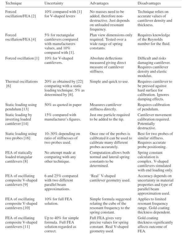
Firstly, as is common in AFMs that use microfabricated cantilevers, the oscillator is held at an angle with respect to the surface, as sketched in figure 1(a). The unit vector that represents the oscillatory motion, xˆ, lies at an angle θ with respect to the direction of motion of the scannerzˆ, the angleθ being the angle of repose of the cantilever with respect to the horizontal. For a given sample movement in thezˆdirection, the cantilever must move a distancex =z/cosθin thexˆ
direction.
Secondly, because any error in the amplitude measurement is squared, limiting the accuracy of the stiffness, the movement of the scanner in the ˆz direction should be verified, and if necessary corrected using interferometry. The cantilever can be placed near a reflective surface and the laser light purposefully placed half on and half off the cantilever. As seen in figure 1(b), the path difference between the two beams isz(1+ cos 2θ). When a force curve is acquired, interference peaks are observed in the data, as is evident in figure 1(c). The distance between these peaks,zp, should be made to equal
λ/(1 + cos 2θ).
The third correction has already been pointed out by Butt and Jaschke [7]. They calculated the effect of all the oscillation modes of the cantilever on the detected signal under various conditions. When the movement of the cantilever is monitored by reflecting a laser beam from the backside of the cantilever and the end of the cantilever is free, the observed fluctuations need to be multiplied by a factor of three-quarters.
As is common practice, we calibrated the photodiode response by placing the cantilever in contact with a stiff surface and ramping the scanner position in order to find the ratio between the manufacturer’s statedzˆmovementzm
Sample Cantilever Laser beam b) 2Θ Θ Θ Θ Sample a) Cantilever Θ ^ z ^ x Θ ∆z -1 -0.8 -0.6 -0.4 -0.2 0 0.2 0.4 0.6 0 500 1000 1500 2000 2500 Deflection [V]
Relative Scanner Displacement [nm] c)
Figure 1.(a) The unit vectorsxˆandzˆused in the calculations and the angle of reposeθof the cantilever. (b) The difference in path length between the laser light reflected from the backside of the cantilever and the laser light reflected from the surface of the sample,z(1 + cos 2θ). Although the sample is drawn as flat, roughness causes some of the reflected light to reach the photodiode. (c) The cantilever’s deflection as a function of the scanner position before the scanner calibration. The distance between peaks should be 348 nm; it was 313 nm.
positioned or repositioned on a cantilever and upon changing the medium from air to water. Taking this last procedure together with the three corrections, the mean-square cantilever amplitude fluctuations are related to the mean-square voltage fluctuations by x2(ν) = 3 4V 2(ν) z m Vm 2 × λ zp(1 + cos 2θ) 2 1 cosθ 2 . (10)
The cantilever’s angle of repose was 11◦ from the horizontal, and the wavelength of the laser was 670 nm. The distance between the interference peaks should be 348 nm; uncorrected, it was 313 nm. Thus for this instrument
x2(ν) =0.962V2(ν) zm Vm 2 . (11)
Ten different Si3N4and Si cantilevers of various shapes
were examined using the four techniques in air and in water. The plan dimensions of the cantilevers were determined with a calibrated optical microscope. For triangular cantilevers, the dimensions were determined in the same manner as [13]. Error-signal images in ‘contact mode’ with zero scan range and zero gains were acquired while the cantilever was hanging freely. These images of the system noise were Fourier transformed and the power spectra [20], measured mean-square amplitudes as a function of frequency, were saved in ASCII format. A spreadsheet program corrected them using equation (11) and fitted them to the sum of three functions [23]:
a 1/f noise background, a white-noise floor and the mean-square amplitude (equation (6) divided by two and multiplied byν, which for this instrument was 122 Hz).
x2(ν) = A ν +B+ x2(ν k) Q2 1 1−νν k 22 +νν kQ 2. (12)
The fit parameters were A, B, x2(ν
k), Q and νk. From
equation (6) or (9), the mean-square amplitude at kinetic resonance, x2(ν
k), equals kBT Qν/πkνk. The kinetic
resonant frequencyνk and the quality factor Qwere used in
calculating the Cleveland and Sader values fork. For the Hutter and Bechhoefer method (equation (5)) the square amplitudes at each frequency were summed to obtain x2, and for our
approach (equation (9)) the values of the amplitude squared at kinetic resonance were determined.
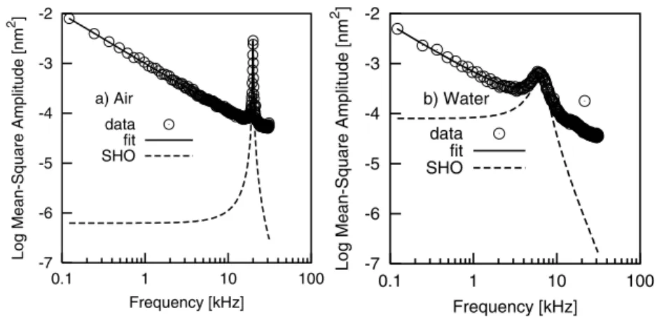
Typical mean-square amplitude distribution spectra for air and water are displayed in figure 2. Both are from the same force-calibrated cantilever (FC2) purchased from TMMicroscopes [24]. Along with the original data set (circles), the fits to the data are shown (solid curves), and as well, the curves after noise contributions had been subtracted out (dashed curves).
4. Results
Table 2 lists the cantilever, the manufacturer’s nominal stiffness, the material from which the cantilever was fabricated, its shape, plan-view dimensions, the medium in which the measurement was made, the cantilever’s quality factor, resonant frequency, square amplitude at resonance and calculated stiffness values for the Cleveland, Sader, and Hutter and Bechhoefer methods, as well as our new approach.
Comparing the values for stiffness obtained in air to the manufacturers’ nominal values, there are variations using the Cleveland method by up to factor of thirteen, for the Sader calculation by up to a factor of four and for the thermal methods by up to factor of three. Comparing the stiffness values for water with those for air within each technique, where one expects identical values, Cleveland’s method is clearly inappropriate for water. The variations are by factors of up to 120 and are probably due to geometry-dependent mass loading by water. The Sader air values range from 15 to 35% lower than the water values for rectangular cantilevers and are 25– 40% lower for triangular ones. For the thermal methods the air results run from 60% higher to 20% lower than the water results.
Comparing the stiffnesses among the techniques, the agreement between Hutter and Bechhoefer’s summation and our new approach using the square amplitude at resonance is within 2%, in both air and water. The thermal measurements yield stiffnesses up to a factor of five different from Cleveland’s approach. The thermal values in air for rectangular levers are from 20% lower to 40% higher than Sader values. In water, they range from 20 to 40% lower than those of Sader. Concerning the force-calibrated cantilevers, the various approaches yield results within 17% of the nominal value in air. Here the Cleveland method gives numbers within 5% of the nominal. There should be a good match; the nominal values were calculated with the Cleveland method by the manufacturer.
-2 -3 -4 -5 -6 -7 0.1 1 10 100
Log Mean-Square Amplitude [nm
2 ] Frequency [kHz] a) Air data fit SHO -2 -3 -4 -5 -6 -7 0.1 1 10 100
Log Mean-Square Amplitude [nm
2 ] Frequency [kHz] b) Water data fit SHO
Figure 2.Mean-square fluctuations in amplitude as a function of frequency for the same force-calibrated cantilever (FC2 in table 2) (a) in air and (b) in water. The circles are the original data, the solid curves the fit to the data including 1/fand white-noise contributions and the dashed curves the contribution of the SHO, that is, the fit minus 1/fand white noise. In (b), a noise spike appears at approximately 22 kHz. The residual root-mean-square error between the solid curve and the data is 2.9×10⁻⁵nm2for the case of air, 1.7×10⁻⁵nm2for water.
Table 2.Summary table of the results for ten different cantilevers. The last four columns contain the spring constants as determined by the four methods under study.
Dimensions k b
nom Frequency x2(νk) kClevelandf kSad er kH&B kN ew Probe (N m−1) Materialc Typed l(µm) w (µm) Mediume Q (kHz) (nm2) (N m−1) (N m−1) (N m−1) (N m−1) FC1a 0.28 Si R 398 33 A 70.1 19.93 0.0035 0.2944 0.2627 0.3255 0.3248 W 2.5 6.55 0.0006 0.0105 0.3067 0.2133 0.2127 FC2a 0.28 Si R 385 32 A 66.6 20.49 0.0032 0.2810 0.2455 0.3286 0.3282 W 2.5 6.72 0.0007 0.0099 0.2990 0.1812 0.1806 FC3a 0.28 Si R 392 33 A 67.3 19.98 0.0031 0.2830 0.2493 0.3466 0.3461 W 2.7 6.47 0.0009 0.0096 0.3136 0.1546 0.1542 5 0.02 SN R 175 19 A 17.4 12.02 0.0402 0.0035 0.0103 0.0115 0.0115 W 1.3 2.83 0.0180 45u 0.0135 0.0081 0.0081 6 0.02 SN R 175 19 A 13.8 9.17 0.0620 0.0015 0.0058 0.0078 0.0078 W 1.2 1.96 0.0316 15u 0.0076 0.0063 0.0062 7 0.02 SN R 175 19 A 18.2 12.02 0.0542 0.0035 0.0108 0.0089 0.0089 W 1.3 2.79 0.0176 43u 0.0131 0.0084 0.0083 9 0.05 SN T 170 19 A 24.2 16.54 0.0131 0.0156 0.0321 0.0357 0.0356 W 1.7 3.76 0.0045 184u 0.0429 0.0329 0.0327 2 0.03 SN T 190 20 A 13.8 10.99 0.0303 0.0071 0.0127 0.0133 0.0133 W 1.3 2.37 0.0182 71u 0.0206 0.0098 0.0097 B 0.03 SN T 185 20 A 18.5 11.76 0.0360 0.0080 0.0181 0.0140 0.0140 W 1.6 2.41 0.0130 69u 0.0257 0.0167 0.0166 C 0.03 SN T 185 20 A 17.3 11.56 0.0362 0.0076 0.0165 0.0133 0.0133 W 1.5 2.37 0.0156 66u 0.0236 0.0134 0.0132 aForce-calibrated cantilever.
bNominal cantilever stiffness as provided by the manufacturer. cSi, silicon; SN, silicon nitride.
dR, rectangular; T, triangular. eA, air; W, water.
fu, microNewtons per metre.
5. Discussion
As seen in figure 2, the fits to the data are very good. The quality factor and resonant frequency in water are much lower than in air. The quality factor decreases due to the high damping of the medium, and the resonant frequency goes down because of mass loading. The low-frequency limits in amplitude are different, and according to equation (6) the low-frequency limit is x2(0) ν = kBT πνkQk , (13)
from which the ratio of the low-frequency limits in water and air is x2 water(0) xair2 (0) = νair k Qair νwater k Qwater . (14)
The quality factors from the data shown in figure 2 are 70 and 2.5 respectively for air and water. The resonant frequencies are 20 and 6.5 kHz. We then expect the ratio of the low-frequency limits to be approximately 100, which is corroborated by the figure, where the dashed curves intersect the y axes at 3.5×10⁻⁷and 4.5×10⁻⁵nm2. The model appears to be an
Each of the four methods has its disadvantages and advantages. The Cleveland method seems to work well for silicon, because the elastic modulus and density of silicon is easily controlled and well known, whereas for silicon nitride those parameters vary. Sader’s method is independent of the material properties, yet dependent on the cantilever’s geometry. Although Sader’s method is technically limited to rectangular beams, we did not find a large variation from the expected values for the triangular cantilevers. The advantage of these two geometric methods is that the sensitivity of the photodiode to the movement of the cantilever does not have to be calibrated. It is sufficient to know the resonant frequency (for both approaches) and the quality factor (for Sader).
Two attractions to the thermal methods are that they are based on standard physics and that they are independent of both the constituent material of the cantilever and its shape. The initial difficulty is that the detector must be calibrated to the movement of the beam. However, this is a common procedure done routinely for force curve acquisition. This calibration will determine the accuracy of the thermal methods, which we estimate to be 20%. One might think that the thermal methods would be susceptible to mechanical noise, but if this were true in our measurements higher values of the amplitude would be expected, yielding small values of stiffness. This was not observed. Depending on the set-up, the thermal methods may be limited by noise such that the peaks are obscured, or by bandwidth, such that only a narrow frequency range can be examined. For example, when acquiring a 512 × 512 noise image at 61 lines s−1, the bandwidth for frequency is
31 kHz. If this bandwidth is too narrow, the error signal may be directly monitored with a wide-bandwidth spectrum analyser or collected by a computer and Fourier transformed.
The Hutter and Bechhoefer method requires that the square amplitude be summed over a large frequency range, and if the resonance occurs near the high end of the available bandwidth then the sum is prematurely truncated. We recommend that for the Hutter and Bechhoefer method the peak should not occur at a frequency much higher than half the bandwidth. Our new method has the advantage that only the resonant frequency, the quality factor and the square amplitude at resonance need to be known, and as such the peak could be near the upper edge of the bandwidth with no ill effects. Another advantage of the new approach is that it can be applied without noise subtraction to data collected in air, because the resonant peaks can be sufficiently high above the noise such that noise subtraction has no noticeable effect (compare figures 2(a) and (b)). Indeed, our choice of methods is the new one.
6. Conclusions
The four cantilever calibration methods investigated in this study agreed within 17% of the manufacturer’s nominal value for well-defined rectangular silicon cantilevers. The
agreement for silicon nitride cantilevers was significantly worse, particularly for the Cleveland method. The new thermal method demonstrated here gives stiffnesses within 2% of Hutter and Bechhoefer’s thermal approach and is similarly independent of cantilever geometry and materials. It also can be carried out in a few minutes with little or no additional equipment, has a more relaxed requirement for bandwidth, is based on important fundamental physics and, hence, is our preferred method.
Acknowledgments
The support of XC from the BBSRC Bioimaging Initiative is gratefully acknowledged, as well as F L Hutson’s criticism of the manuscript.
References
[1] Cleveland J P, Manne S, Bocek D and Hansma P K 1993Rev. Sci. Instrum.64403–5
[2] Sader J E, Larson I, Mulvaney P and White L R 1995Rev. Sci. Instrum.663789–98
[3] Sader J E 1998J. Appl. Phys.8464–76
[4] Sader J E, Chon J W M and Mulvaney P 1999Rev. Sci. Instrum.703967
[5] Chon J W M, Mulvaney P and Sader J E 2000J. Appl. Phys.
873978–88
[6] Hutter J L and Bechhoefer J 1993Rev. Sci. Instrum.64
1868–73
[7] Butt H-J and Jaschke M 1995Nanotechnology61–7 [8] Neumeister J M and Ducker W A 1994Rev. Sci. Instrum.8
2527–31
[9] Hazel J L and Tsukruk V V 1996Polym. Preparation37
567–68
[10] Hazel J L and Tsukruk V V 1998J. Tribol.120814–19 [11] Hazel J L and Tsukruk V V 1999Thin Solid Films339249–57 [12] Stark R W, Drobek T and Heckl W M 2001Ultramicroscopy
86207–15
[13] Butt H-J, Siedle P, Seifert K, Fendler K, Seeger T, Bamberg E, Weisenhorn A L, Goldie K and Engle A 1993J. Microsc.
16975–84
[14] Senden T J and Ducker W A 1994Langmuir101003–4 [15] Holbery J D, Eden V L, Sarikaya M and Fisher R M 2000Rev.
Sci. Instrum.713768–76
[16] Gibson C T, Watson G S and Myhra S 1996Nanotechnology7
259–62
[17] Tortonese M and Kirk M 1997SPIE300953–60
[18] Pathria R K 1972Statistical Mechanics(Oxford: Pergamon) [19] Atkins P W 1978Physical Chemistry(San Franciso, CA:
Freeman)
[20] Ramirez R W 1985The FFT, Fundamentals and Concepts (Englewood Cliffs, NJ: Prentice-Hall)
[21] MacDonald D K C 1962Noise and Fluctuations: an Introduction(New York: Wiley)
[22] Svoboda K and Block S M 1994Annu. Rev. Biophys. Biomol. Struct.23247–85
[23] Walters D A, Cleveland J P, Thomson N H, Hansma P K, Wendman M A, Gurley G and Elings V 1996Rev. Sci. Instrum.673583
[24] TMMicroscopes Cantilever Order Center. http://spmprobes.com