ARLib: A C++ Augmented Reality Software Development Kit. Masters Thesis

ARLib: A C++ Augmented Reality

Software Development Kit

Masters Thesis

Daniel Diggins

MSc Computer Animation

N.C.C.A Bournemouth University

Contents

1

Introduction ... 3

2

Previous and Current Work ... 5

3

Image Segmentation... 7

3.1 Static Thresholding ...7

3.2 Dynamic Thresholding ...8

4

Feature Extraction ... 12

4.1 Detecting the Corners...12

4.2 Detecting the Marker Edges ...15

4.3 Custom Corner Detector...20

5

Marker Detection... 23

5.1 Detecting Markers...23

5.2 2D-to-2D Projection Mappings...24

5.3 Detection Problem ...28

6

Camera Orientation... 30

7

Using ARLib ... 35

7.2 The “Hello World” ARLib Application ...35

7.3 Running an ARLib Application ...37

7.4 Adjusting for Varying Lighting Conditions ...37

7.5 A Custom ARLib Application...38

8

Conclusion ... 43

8.1 Recommendations...43

Appendices ... 45

Appendix A Sample Otsu Thresholding C++ code ...45

Appendix B ARLib Application Command-Line Switches ...46

Appendix C ARLib Application User-Interface Keys ...47

Appendix D ARLib Configuration File ...48

1

Introduction

Computer Graphics is now a huge industry. Computer Graphics (CG) applications are now used across a wide range of industries, including the more obvious, such as film and TV, manufacturing and the defence sector, through to the less well known such as specialist medical units.

CG has dominated the film industry in recent years, with a greater proportion of movies being made that use computer generated special effects compared with those that contain none at all. Even movies that look as if they have no special effects are likely to have been digitally manipulated or enhanced in post-production. From a director’s point of view, the use of computer graphics gives an endless creative power, in what would normally be an impossible shot to make. The downside is that the cg elements have to be added after the scenes have been shot, a process that can take many months to complete. It is not until the cg and live action footage are merged together that the final result can be viewed and is hopefully how the director envisaged it.

The ability of computers to handle complex tasks has grown in parallel with their processing power and, in particular, their ability to perform graphically intensive operations in real-time has improved so much that previously impossible cg scenarios are now both feasible and commonplace.

An exciting development within the computer graphics arena is the field of

Computer Vision. This is the ability of a computer to be able to recognise key points or extract specific features from both still images and video footage. The use of Computer Vision for reading still images is used in optical character recognition (ocr), where a computer is able to translate handwritten characters into computer text. Facial recognition is another commonly used area of computer vision with still images. However, recognition of moving images is a much less developed field. One such example is a police pedestrian monitor, used to identify potential criminals by their unlawful activities [DAVIES 2005].

Augmented Reality is a fast growing field within Computer Vision, where the use of computer graphics and live footage has taken advantage of the advances in processing power. Augmented Reality is a process in which computer graphics are placed over live footage so that the cg elements look as if they are integral to the scene. The use of Augmented Reality could, in the not too distant future, help directors to visualise how the computer graphic elements will interact in the scene during the actually shooting.

This Masters Thesis describes the process of developing an Augmented Reality C++ development kit called ARLib. The ARLib toolkit enables developers to create Augmented Applications quickly and easily. The applications work by looking for predefined black and white markers in the video footage and then placing computer graphics over the top of them. The entire process has been broken down into separate modules, each one handling a specific task.

As a means of placing this AR toolkit into context within the AR marketplace,

Chapter 2 details how AR applications are being used today, and by whom.

Chapters 3-6 cover how the ARLib was developed, and what models and methods were used in its implementation.

Chapter 3 describes the first stage of performing Augmented Reality by taking a colour image and converting it to black and white so that features within it can be detected.

Chapter 4 details the process of extracting useful features, ie; black and white markers, from the black and white image.

Potential markers in an image are then further analysed to determine whether it is a valid marker. This process is described in Chapter 5.

The final stage of the Augmented Reality process involves determining where the marker is in relation to the camera and is detailed in Chapter 6.

Chapter 7 describes how to create applications using ARLib. The C++ code for two working examples is detailed, which are included as part of ARLib.

Finally, the conclusion and recommendations for further developments are discussed in Chapter 8.

2

Previous and Current Work

A key aspect of Computer Vision is the ability of the application to identify known entities within an image. Some techniques for performing computer vision use markers to aid in the recognition process whereas more recently markerless detection systems have been developed [VACCHETTI et al 2003], [ALLEZARD et al 2000] and [LEPETIT 2004]. These markerless systems still require some knowledge about the environment. Some techniques use a computer model of an object to use as a template, where lines and features detected in the scene are matched against the model’s shape. Other techniques search for textures on objects.

The application of Augmented Reality within the realms of Computer Vision is becoming more common and is now used in many different fields, including medical, manufacturing, military and visualisation. In particular, fighter pilots have been using the application of augmented reality for many years to highlight the outside world in the form of head up displays.

The University of North Carolina has researched into using augmented reality in medicine [LIVINGSTON 1998] as an aid for performing surgery, see figure 2.1.

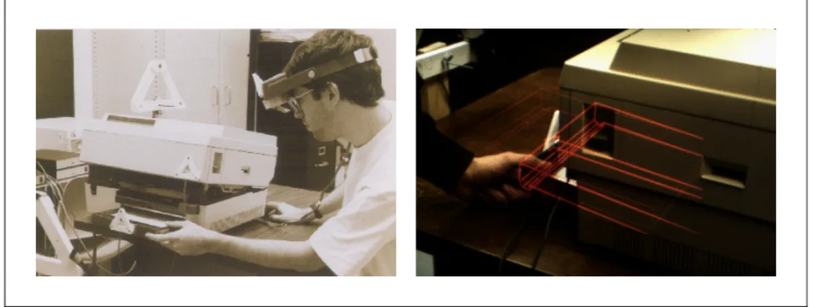
Another interesting example of Augmented Reality is an application that was developed to aid maintenance engineers who have to repair a variety of different equipment [FEINER 1993]. The system works by incorporating a camera into the engineer’s goggles, which is linked to the AR software. The AR application is able to annotate what the engineer is seeing with useful text and markers, to aid the engineer in his job, see figure 2.2.

Figure 2.2Using Augmented Reality to Assist Maintenance Engineers

A mundane but essential task of quality control has been made easier by AR. Custard creams are scanned for excess cream by an AR application and rejected if they fall outside of a predefined limit [DAVIS 2005].

L'Ecole Polytechnique Fédérale de Lausanne (EPFL) is a Swiss University that has a dedicated computer vision lab. Within this lab they have developed many techniques and applications in the realms of augmented reality, including real-time face tracking and 3D object tracking.

Figure 2.3 Examples of EPFL’s AR Work

It is EPFL’s 3D object tracking work that inspired the development of the ARLib, and is described in detail in the following chapters.

3

Image

Segmentation

With most applications of computer vision, one of the primary and most important tasks is to isolate the foreground from the background objects. This task is often referred to as segmentation or thresholding and its performance in isolating elements will determine how successful features can be extracted from the image.

3.1 Static

Thresholding

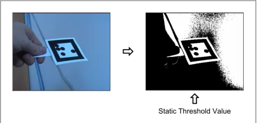
This is the simplest and most basic form of segmentation that takes the grey value of each pixel and converts it to black or white, depending on a static threshold value. Figure 3.1 shows the flow of the basic segmentation technique.

Ö

×

Static Threshold Value Figure 3.1 The basic segmentation technique

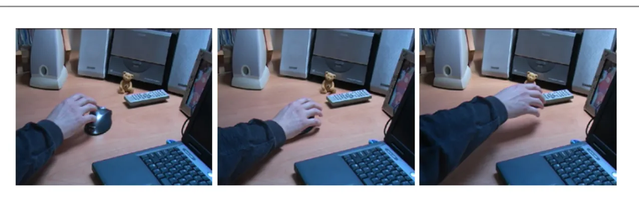
Under ideal circumstances, where the lighting and camera parameters are constant, the basic segmentation technique will perform adequately for most tasks. However, most captured video images are susceptible to noise and fluctuations in brightness and will therefore produce varying levels of segmentation. To demonstrate this, figure 3.2 shows three images taken from a static video camera. Although the background elements appear to be the same, by comparing the differences it can be seen in figure 3.3 that there were varying levels of brightness even in static regions.

Figure 3.2 Captured Video Images

Figure 3.3 Varying brightness levels for static objects.

When dealing with a single image, a static threshold value will suffice, as the value can be adjusted manually to get the desired segmented image. For video sequences, manual adjustment of the threshold value is an impractical solution as the images are being processed at a rate of 25 frames per second and therefore a technique was required that will automatically adjust the threshold from frame to frame.

3.2 Dynamic

Thresholding

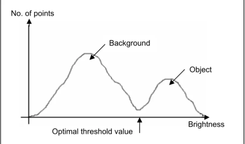
Also known as optimal thresholding, dynamic thresholding attempts to calculate the optimal threshold value based on the grey level values of the image. Each frame of an image sequence is analysed and a threshold value is calculated. This has the advantage that, if the luminance of the sequence is inconsistent between frames, then the dynamic threshold value should stabilise the problem. One of the more popular approaches of dynamic thresholding is the Otsu Method [NIXON and AGUADO 2002]. The Otsu method works on the theory that there are two peaks in the grey values of an image’s histogram, one representing the

background and the other representing either the foreground or an object. Otsu makes the assumption that the lowest mid-point between these two peaks is the optimal threshold value, see figure 3.4.

Figure 3.4 Otsu optimal threshold position

Ö

Ö

Colour Image Grey level histogram Dynamic threshold Figure 3.5 The Otsu Thresholding technique

The optimal threshold value is calculated from the Otsu method using the following equations:

∑

=

l

p

k

)

(

)

(

ω

∑

⋅

=

l

p

l

k

)

(

)

(

μ

∑

⋅

=

)

(

l

p

l

T

μ

Using the previous equations, the final calculation can be expressed as:

))

(

1

)(

(

))

(

)

(

(

)

(

k

k

k

k

T

k

ω

ω

μ

ω

μ

σ

−

⋅

⋅

=

k = The histogram index position in the range 0 to 255.

p = The normalised histogram value for the current index position.

ω and μ = The first and second order cumulative values of the normalised histogram.

μT = The total mean level of the image.

See Appendix A for example C++ implementation code for the Otsu thresholding method.

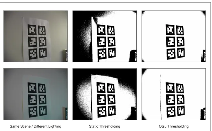
A final comparison of how Otsu’s algorithm performed against a static threshold is shown in figure 3.6. The first column shows the same scene with different lighting. The middle column shows the result after using a static threshold value and the third column shows the result with the Otsu dynamic thresholding method. It can clearly be seen that the Otsu method out-performed the static method, as the markers were more pronounced and also the noise caused from the shadows was greatly reduced.

Same Scene / Different Lighting Static Thresholding Otsu Thresholding

4

Feature

Extraction

Feature extraction is a term used for finding known elements within an image. These elements consist mainly of corners, lines, shapes and curves. The ARLib uses two dimensional square markers for its detection system, therefore the features required were corners and edges.

4.1 Detecting the Corners

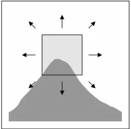
There is a variety of corner detection algorithms documented in many textbooks and research papers. A commonly used method is the Harris Corner Detector [HARRIS and STEPHENS 1988]. The basic mechanism behind the Harris detector is that a small square template window is centred on a point in the image. The template window is then slightly shifted in various directions and the average change in intensity is recorded. It is these changes in intensity that can indicate whether the template window is on a corner, see figure 4.1.

Figure 4.1 The Harris Corner Detector

Although deemed to be the preferred method for detecting corners, it was estimated that the algorithm would take too much computation time and would hinder the real-time target of ARLib.

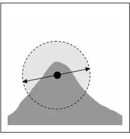
Another common technique for detecting corners is known as the SUSAN Corner Detector [SMITH and BRADY 1997]. This technique uses a circular template mask which is placed over every pixel in the image. All pixels of a similar intensity to the central pixel are counted, and if the count is less than half of the number of pixels in the template, then it is assumed a corner exists within the

circle. The actual location of the corner is indicated by performing a local minimum search within the template area, see figure 4.2.

Figure 4.2 The Susan Corner Detector

Initial prototyping and testing showed that the SUSAN algorithm was too slow at processing to be used in a real-time application.

Another corner detection algorithm that uses a circular template is detailed in [EPFL 2004] and is referred to as the Keypoint Detector. This technique differs from the SUSAN method in that only the pixels on the circumference of the template are analysed. The idea behind this technique is that if two diametrically opposed pixels have a similar intensity to the central pixel, then the point is not a corner or feature point, see figure 4.3.

Figure 4.3 The Keypoint Detector

Because of the way video images get digitised, some straight edges can be falsely recognised as corners. To overcome this problem, the neighbouring cells on the circumference are also tested, see figure 4.4.

Figure 4.4 Testing Neighbouring Pixels in Keypoint Detector

This algorithm was initially implemented in ARLib as it performs well and has no real noticeable affect on performance. Figure 4.5 shows some sample video images with highlighted corners. It can be seen that there appeared to be more corners indicated than were actually visible. This was due to noise caused by the segmentation process.

4.2 Detecting

the Marker Edges

When a two dimensional square is viewed from any angle, its edges always remain straight, therefore if the four edges of the square can be detected, then its corners can also be calculated using simple line intersection routines.

Since its invention in 1962 by Paul Hough, the Hough transform method [DUDA and HART 1972] has been the main technique used for detecting lines within an image. The technique has been further advanced to detect arbitrary shapes and is called the Generalised Hough transform.

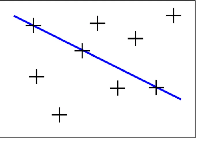
The principle behind the Hough transform is that there are an infinite number of lines that can pass through a single point. However, if many collinear points are examined, then there is only one line that is common to all of them, see figure 4.6. It is this simple concept that is used by the Hough transform.

Figure 4.6 The Hough transform principle

The original method for calculating the lines in the Hough transform used the slope-intercept equation of:

c

mx

y

=

+

Here a range of values are used for m and c to determine the lines for a particular point (x,y). A major problem with using the slope-intercept technique is that there is no way of knowing the range of values to use for m and c.

Another technique was tried [DAVIS 2005] that replaced the slope-intercept formula with one called the normal(θ,p) form:

)

sin(

)

cos(

θ

+

⋅

θ

⋅

=

x

y

p

Using this formula, the lines were represented using a sinusoidal wave. Points were plotted and multiple hits in (θ, p) space indicated the presence of a line. Multiple hits are highlighted in figure 4.7.

Figure 4.7 Hough Transform Sinusoidal Wave.

The Hough transform is a very accurate technique for detecting lines within an image and functions well in noisy images too. It is, however, very computationally expensive and it is this reason that the Hough transform was not used in ARLib, as it cannot perform satisfactorily in a real-time scenario.

With the combination of these two problems, ie; the Hough transform not performing well and the corner detection not picking up all corners, another more efficient and reliable technique was needed.

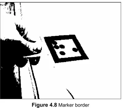
In [MALIK 2002], a completely different approach is used to detect the corners and edges of the markers. The technique takes advantage of the fact that a marker comprises of a thick black border that is surrounded by a white edge, see figure 4.8.

Figure 4.8 Marker border

It can be seen that a potential marker’s boundary consists of a large connected region of black. To identify these regions, bounding boxes were created around the black border.

Looking for the black regions was a fairly simple process and the well known flood-fill technique [FOLEY et al 1990] was used. During the flood-fill process, the current bounding box was adjusted accordingly, see figure 4.9.

The process is described in the following steps:

1. Starting at the bottom-left pixel of the image, each row is scanned until a black pixel is found.

2. When a black pixel is found, it is flagged as being processed and a bounding box is created around it.

3. The four unprocessed neighbouring pixels (above, below, left and right) are recursively scanned and processed and the extents of the bounding box are adjusted accordingly.

4. When no more black pixels can be found during the recursive process, the current bounding box is added to the list of regions that may potentially contain a marker.

5. The scanning of rows continues until another unprocessed black pixel if found, then steps 2 to 4 are repeated.

Figure 4.10 Example bounding boxes

Because there is noise in an image, the number of bounding boxes could potentially be large, which would hinder the performance of the detection process. The problem was easily overcome by applying some simple checks prior to each bounding box being added to the current list:

1. If the bounding boxes area is smaller than a predefined value then it is deemed too small for processing and is excluded, see figure 4.11a.

2. If the aspect ratio of the box is below a defined threshold, then the assumption is made that either the region does not contain a square or, if it did contain a square, then it is being viewed from too sharp an angle for a satisfactory detection, see figure 4.11b.

Figure 4.11 Bounding Box Exclusions. (a) Area and (b) Aspect Ratio too small.

Within each bounding box, a convex hull exists defined by the maximum extents of the black pixels. Because the markers were square, then the convex hull should contain four corners, see figure 4.12.

Figure 4.12 Bounding Box and Convex Hull can help identify corners.

In [MALIK 2002], the assumption is made that a straight edge consists of approximately 50% black and 50% white pixels, while the corner has more than 50% white. To determine if an edge is a corner, a square template is placed centrally over the edge pixel. A count is then made of the black and white pixels and the four highest scoring counts are recorded. This entire corner detection process is included in the recursive flood fill routines.

The results from the corner detection process proved successful for most cases in ARLib but, like many corner detection routines, they performed best when the image being processed contained a marker that was relatively flat within the scene. Testing of this technique revealed that the corners were not detected when the marker was at an angle to the camera. This is because, in some instances, a corner can look almost like a straight edge, see figure 4.13.

Figure 4.13 Corners appearing as a straight edge.

Further research failed to reveal an alternative corner technique that was capable of overcoming this problem therefore a custom corner detection method was devised and implemented.

4.3 Custom Corner Detector

A technique was needed for ARLib that would reduce or even take away the assumptions of other corner detection routines, in which a corner was determined by the ratio of black to white pixels. Because the bounding box and outer edges of the black region within the box are known, a geometric solution was possible. If a bounding box was scaled so that it forms a square, then this simplified the problem even further, see figure 4.14.

Figure 4.14 Scaling bounding boxes to form a square.

Once the bounding box was a square, the region corners could be identified by working out the furthest edge pixel from each of the bounding box corners, see figure 4.15.

Figure 4.15 Detecting region corners from bounding boxes.

Although this technique succeeded where previous detectors had failed i.e. it detected almost straight corners, this technique also had a problem with one particular scenario. The corners were not detected correctly when the region within the bounding box formed a diamond shape. The problem was caused because two of the corners in a diamond shape were the same distance from two of the bounding box corners, therefore only two corners were detected, see figure 4.16.

Figure 4.16 Two corners detected when diamond shape.

A simple solution to the problem was that, if four unique corners were not detected using the four corners of the bounding box, then four alternate points on the bounding box were used. In this case, the mid-point of each of the corners were used, see figure 4.17. By using both sets of bounding box reference points, it guaranteed that fours corners were always found.

5

Marker

Detection

A 2D marker or fiducial, as it often called, must be designed in such a way that can be easily detected and be unique enough to be easily identified from other markers. Each marker must also provide some kind of unique binary code so that its ID can determined. Most markers use black and white designs, however in [EPFL 2004] a technique is described that can be used on detailed coloured markers by using classification trees for identification.

In ARLib, black and white markers were used and were based initially on the design in [LIU et al 2002], however as will be shown, this design did not perform well at acute angles.

The marker design uses a 5x5 matrix where each cell represents a single bit in the marker’s identification code, see figure 5.1.

Figure 5.1 5x5 Matrix Design

This marker represents a 25 bit binary code. 12 of the bits are used for the actual marker ID. The four corners are used to determine the orientation and the remaining bits are used for error detection. The error detection bits enable falsely detected markers to be rejected.

5.1 Detecting

Markers

Detecting a potential marker in ARLib involved finding the location and colour of each cell within the image. Because the corners of the marker were available, the problem was simplified to mapping a square to a quadrilateral, see figure 5.2.

P1 P1 P1

P1

P2 P2 P2

P2 P1

P2

Orientation bit (4 bits)

Marker code bit (12 bits)

Parity code for rows (4 bits)

Figure 5.2 Mapping a square to a quadrilateral.

A solution is described in [HECKBERT 1995] and is commonly called projective mapping. The technique is often used in computer graphics when performing texture mapping. Projective mappings can be performed in 3D, but for the purposes of ARLib, 2D projections were used.

5.2 2D-to-2D

Projection

Mappings

The main principle behind projective mapping is to take points from one plane and project them onto another.

The general form for a projective mapping is:

i

hv

gu

c

bv

au

x

+

+

+

+

=

i

hv

gu

f

ev

du

y

+

+

+

+

=

These previous two equations can be represented in homogeneous form as:

⎥

⎥

⎥

⎦

⎤

⎢

⎢

⎢

⎣

⎡

⋅

⎥

⎥

⎥

⎦

⎤

⎢

⎢

⎢

⎣

⎡

=

⎥

⎥

⎥

⎦

⎤

⎢

⎢

⎢

⎣

⎡

i

h

g

f

e

d

c

b

a

q

v

u

w

y

x

By solving the above unknowns a-i, then by specifying u and v coordinates in the reference square, the x and y coordinates in the quadrilateral can be calculated, see figure 5.3.

Figure 5.3 u/v to x/y coordinates.

In the homogeneous matrix of the problem, assuming i=1, then there are eight unknowns. By using the four corners of the reference square and the four corners of the quadrilateral, then eight equations can be defined. Each corner mapping produces the following equations:

k k k k k k k k k k k k

u

a

v

b

c

u

x

g

v

x

h

x

hv

gu

c

bv

au

x

⇒

+

+

−

−

=

+

+

+

=

k k k k k k k k k k k k

u

d

v

e

f

u

y

g

v

y

h

y

hv

gu

f

ev

du

y

⇒

+

+

−

−

=

+

+

+

=

The eight equations can be written using an 8x8 system for k=0 to 3:

⎥

⎥

⎥

⎥

⎥

⎥

⎥

⎥

⎥

⎥

⎥

⎦

⎤

⎢

⎢

⎢

⎢

⎢

⎢

⎢

⎢

⎢

⎢

⎢

⎣

⎡

=

⎥

⎥

⎥

⎥

⎥

⎥

⎥

⎥

⎥

⎥

⎥

⎦

⎤

⎢

⎢

⎢

⎢

⎢

⎢

⎢

⎢

⎢

⎢

⎢

⎣

⎡

⋅

⎥

⎥

⎥

⎥

⎥

⎥

⎥

⎥

⎥

⎥

⎥

⎦

⎤

⎢

⎢

⎢

⎢

⎢

⎢

⎢

⎢

⎢

⎢

⎢

⎣

⎡

−

−

−

−

−

−

−

−

−

−

−

−

−

−

−

−

1

0

0

0

1

0

0

0

1

0

0

0

1

0

0

0

0

0

0

1

0

0

0

1

0

0

0

1

0

0

0

1

y

y

y

y

x

x

x

x

h

g

f

e

d

c

b

a

y

v

y

u

v

u

y

v

y

u

v

u

y

v

y

u

v

u

y

v

y

u

v

u

x

v

x

u

v

u

x

v

x

u

v

u

x

v

x

u

v

u

x

v

x

u

v

u

The linear solution can be solved using Gaussian elimination or by calculating the inverse of the 8x8 matrix. The downside of solving the above solution is that it it computationally expensive, however this solution handles the mapping of a general quadrilateral to another quadrilateral. For ARLib, all that was required was to map a square to a quadrilateral therefore the solution could be simplified. Assuming the square to quadrilateral vertex correspondences were as follows:

x y u v

x0 y0 0 0

x1 y1 1 0

x2 y2 1 1

Then the eight equations could be reduced to: 2 1 2 1 2 2

/

y

y

x

x

y

y

x

x

g

Δ

Δ

Δ

Δ

Δ

Δ

=

∑

∑

/

y

y

x

x

y

y

x

x

h

Δ

Δ

Δ

Δ

Δ

Δ

=

∑

∑

x

gx

x

a

=

−

+

d

=

y

−

y

+

gy

x

hx

x

b

=

−

+

e

=

y

−

y

+

hy

x

c

=

f

=

y

x

x

x

=

−

Δ

Δ

y

=

y

−

y

x

x

x

=

−

Δ

Δ

y

=

y

−

y

∑

x

=

x

−

x

+

x

−

x

∑

y

=

y

−

y

+

y

−

y

Using the solved projection mapping equation, it was now a straight forward task to determine the colours of the cells within the potential marker.

The u and v coordinates were divided up into the number of columns and rows and then the central position of each column and row was used to locate the point in the image, see figure 5.4.

5.3 Detection

Problem

The marker design described above had some problems in that detection performed poorly as the marker was moved away from the camera, which was amplified when the marker was also at an angle. After a variety of experiments, the markers were redesigned to use large circles instead of square cells. The bits used for error detection were removed to allow more space for the larger circles, see figure 5.5. Using a circle improved marker detection, even at acute angles.

Figure 5.5 New marker design using circles.

In the original marker design, all cells were scanned during the detection process, whereas in the new design only cells that should be definitely black or white were tested, for example figure 5.6 shows how the marker shown in figure 5.5 was defined.

Figure 5.6 New Marker definition

Using this new approach, in the example above a maximum of 7 checks were needed. 0 1 2 3 4 5 6 7 8 0 1 2 3 4 5 6 7 8 Black Cells White Cells (1 , 3) (3 , 3) (2 , 6) (7 , 5) (5 , 1) (5 , 3) (4 , 6)

6

Camera

Orientation

Once a marker had been successfully identified, the final step in the process was to determine the location of the marker in world space. This step was needed so that, when augmented graphics were rendered on top of the image, their scale and orientation would match the detected marker.

Determining the location of the marker in world space raised some interesting problems. The main one was that the only information available was the 2D coordinates of the reference square and the marker corners. There was also the added complexity in that the marker corners were subjected to perspective. In computer vision, this problem is referred to in many different ways, including Pose Estimation [ABIDI and CHANDRA 1989], Camera Calibration [EASON et al 1984] and Object Pose [LEPETIT 2004]. Although referred to by different names, they each attempt to calculate the camera’s internal and external parameters. The internal parameters, referred to as intrinsic parameters, are the focal lengths in the u and v direction. These two values control the perspective scaling of the augmented graphical objects. The external parameters, called extrinsic parameters, define the camera’s location and orientation with respect to the marker.

Many solutions assume that the focal length is already known and can be substituted into the relevant equations. ARToolkit [KATO 2005] uses this approach and supplies the required tools for calibrating new cameras. For ARLib, a solution was needed that would be able to calculate the focal length automatically. Such a solution is described in [MALIK 2002] in which the mapping of a planar marker in world space is mapped to the image plane, see figure 6.1. It is this technique that was implemented in ARLib.

Figure 6.1 Planar Mapping from world to image space

The 2D to 2D projection matrix calculated in section 4 were used as the starting point. The technique, used in ARLib, calls on the projection matrix values to enable the focal lengths and orientation to be calculated automatically.

The general perspective matrix is show in equation 6.1. This matrix was simplified and shown in equation 6.2.

⎥

⎥

⎥

⎦

⎤

⎢

⎢

⎢

⎣

⎡

=

=

t

r

r

r

t

f

r

f

r

f

r

f

t

f

r

f

r

f

r

f

M

M

M

⎥

⎥

⎥

⎦

⎤

⎢

⎢

⎢

⎣

⎡

=

t

r

r

t

f

r

f

r

f

t

f

r

f

r

f

H

The following rules exist with the H matrix:

1

+

r

+

r

=

r

1

+

r

+

r

=

r

0

r

+

r

r

+

r

r

=

r

Using the rules in equations 6.3 to 6.5, matrix H could then be arranged into two equations for solving fu and fv:

)

(

)

(

)

(

)

(

h

h

h

h

h

h

h

h

h

h

h

h

h

h

h

h

f

−

+

−

−

−

−

−

=

)

(

)

(

)

(

)

(

h

h

h

h

h

h

h

h

h

h

h

h

h

h

h

h

f

−

+

−

−

−

−

−

=

Once the intrinsic values have been calculated from the above equations, the remaining matrix values could be calculated using the following equations:

u

f

h

r

=

λ

/

r

=

λ

h

/

f

r

=

r

r

−

r

r

t

=

λ

h

/

f

f

h

r

=

λ

/

r

=

λ

h

/

f

r

=

r

r

−

r

r

t

=

λ

h

/

f

h

r

=

λ

r

=

λ

h

r

=

r

r

−

r

r

t

=

λ

h

Where λ is a scaling factor and was calculated using the following equation: 2 31 2 2 21 2 2 11

/

/

1

h

f

h

f

h

+

+

=

λ

6.2 OpenGL

Matrices

Once the values had been calculated for fu, fv, r11-r33 and t1-t3, they could then be

used to construct the projection and model view matrices.

To create the projection matrix, the fu and fv value were used in the glFrustum function call.

void glFrustum(GLdouble left, GLdouble right, GLdouble bottom, GLdouble top,

GLdouble zNear, GLdouble zFar)

Typical values used in the glFrustum call were: right = imageWidth / fu

left = -right

top = imageHeight / fv

The model view matrix could be constructed from the remaining values r11-r33 and

t1-t3. The OpenGL function glLoadMatrix uses matrices in column-major order,

therefore the values in ARLib were needed to be transposed from the matrix in equations 6.8 to 6.19. The sixteen elements of the glLoadMatrix parameter were set as follows: M[0] = r11 M[4] = r21 M[8] = r31 M[12] = 0 M[1] = r12 M[5] = r22 M[9] = r32 M[13] = 0 M[2] = r13 M[6] = r23 M[10] = r33 M[14] = 0 M[3] = t1 M[7] = t2 M[11] = t3 M[15] = 1

6.3 Augmentation

Once the OpenGL projection and model view matrices had been initialised, then standard calls to Glut and OpenGL could be made to render 3D objects. Any rendered objects would be positioned and scaled on the marker with the scene. Because there could be multiple markers within a particular image, the whole process of calculating the camera intrinsic and extrinsic parameters needed to be calculated for each marker. The call to glFrustum and the loading of the model view matrix also needed to be carried out for each marker.

7

Using

ARLib

The ARLib toolkit was written for both Windows and Linux. It consists of a single static library that is linked into the final Augmented Reality application.

7.1 Installation

Before applications can be developed using ARLib, the library needs to be built. Linux

ARLib has the following external dependencies and they must be installed prior to building the library:

• Libtiff • Glut • OpenGL

Once these dependencies have been installed, the ARLib static library can be built by typing “Make”. This process creates a file called “libAR.so” in the “lib” folder. The file should be moved either to another location, where it can be located by the linker, or alternatively, the LD_LIBRARY_PATH can be updated to include the lib folder path.

Windows

The Windows version of ARLib has the following dependencies: • Libtiff

• Glut • OpenGL • DirectX 9

A Visual Studio .NET C++ solution file exists within the “vcc” folder. This should be loaded into Visual Studio and built using the “Build” option. The file “AR.lib” will be created in the “lib” folder.

7.2 The

“Hello

World” ARLib Application

To demonstrate the ease of use of ARLib, a basic application is described below. The basic application uses no custom functionality, but has instead all the

features of all AR applications developed using ARLib. Note that the source files for this application can be found in the “examples\BasicApp” folder.

The first requirement of the application is to include the relevant header files:

#include <arlib.h>

#include <arapplication.h>

#include <arappbase.h>

These are the main header files. As more functionality of ARLib is used, then additional files will need to be included.

ARLib uses namespaces to group functional areas. The top level namespace is ARLib and within this namespace, there are the functional namespaces.

using namespace ARLib::Application;

The final piece of code required is the main function.

int main(int argc, char *argv[]) {

ARApplication<ARAppBase> app(&argc, argv); app.Run();

return 1; }

The first line of code constructs an ARApplication variable called “app”. The ARApplication is a template class and therefore requires a template argument. The argument in this case is the ARAppBase class name. This class provides all the base functionality for ARLib applications, including display and user interface operations. This functionality can be changed by specifying a custom class name as the template argument for ARApplication. However, the custom class must be derived from ARAppBase.

The next line of code calls the Run method of the ARApplication. This method puts the application into Augmented Reality mode and will display the specified images or video with computer graphics overlaid.

Once the above code has been written, it can be built, but before it can be executed, there are some additional requirements.

All ARLib applications are configured through external configuration files, so some additional files will need to be created for the basic application.

Fortunately, template versions of these files with default settings are supplied with the ARLib application. The folder “config” should be copied to the location of the final application executable. For details on how to modify the configuration files, see Appendix D.

7.3 Running an ARLib Application

Running the executable without any command-line arguments will attempt to connect to a video source if one is available. In Linux this can be a webcam and in Windows this can either be a webcam or an IEEE1394/firewire device. If no video source is available, a pre-recorded sequence of .tif files can be viewed. To specify a sequence, the following command-line argument should be used:

AppName -sequence <filename>

The filename parameter should be the first image to be used in a numbered sequence of files ie. footage.0001.tif.

As well as displaying sequences of files, a single image can also be viewed:

AppName - image <filename>

For a complete list of available command-line arguments, see Appendix B.

Once the application is running, there are numerous keys that can be used to control the functionality, see Appendix C for a complete list. Some of the more useful keys are:

Tab Toggles between the display of messages and debug information. F Toggles between full screen and windowed mode.

+/- Zoom in and out. Space Pauses the sequence.

7.4 Adjusting for Varying Lighting Conditions

Although the routines used in ARLib attempt to minimise the amount of adjustments required, in varying lighting conditions, they will generally need to be tweaked to get the best results when detecting markers. The main adjustments that will need to be made are in the segmentation process, when the colour image is converted to black and white. The Otsu thresholding technique described in Chapter 3 automatically calculates the relevant values, but does not

cater for the fact that the scene may either be brightly lit or is in low light. Therefore, the Otsu values need to be offset to cater for the current lighting.

The following steps describe the process for adjusting the Otsu thresholding value:

1. Press the ‘A’ key to display the alpha channel of the image. This makes the adjustment easier to see.

2. Press the ‘U’ key to enter update mode. This will display each option that can be updated at the top of the screen. Use the left and right arrow keys to navigate backwards and forwards through the available options.

3. Navigate to the option called “Otsu Threshold Offset” and use the up and down arrow keys to adjust the value until the markers are more pronounced. The ideal setting is to have more white than black, whilst ensuring that the definition of the markers is as clear as possible.

4. Once the Otsu value has been adjusted press the escape key to exit update mode.

5. To switch back into colour mode, press ‘C’.

7.5 A Custom ARLib Application

The basic functionality of ARLib supports the augmentation of static images or models. To add animated effects, a custom implementation needs to be made. To demonstrate how to implement custom code, the “Clock” example (found in “examples\Clock” folder) is described below.

The “Clock” example comprises of three source files, one header file and two implementation files.

clock.h

The clock header file details the custom functionality that will be provided by the Clock class. The first requirement is to include the ARLib headers that will be used:

#include <arappbase.h>

#include <arboundingbox.h>

The next step is to define the class:

class Clock : public ARLib::Application::ARAppBase

All custom implementations must be derived from the ARAppBase class.

The final stage of the class definition is to list the methods that are to be overridden from the ARAppBase class:

public:

virtual void OnGetApplicationTitle( ARLib::Utility::ARString &title );

virtual void OnGetDetailHelp( ARLib::Utility::ARString &help );

virtual void OnInit( int *argc, char *argv[] );

virtual void OnInitDisplayAR();

virtual void OnDisplayAR( ARLib::Detection::ARBoundingBox *marker );

The details behind these methods will be described in the next section. clock.cpp

First define the header files and namespaces that are to be used:

#include <clock.h>

#include <armodels.h>

#include <time.h>

#include <sys/timeb.h>

// specify the ARLib namespaces that are to be used using namespace ARLib::Application;

using namespace ARLib::Graphics;

using namespace ARLib::Utility;

Next define the constant variables that are to be used by the custom implementation:

// define OpenGL colour parameters

const GLfloat ambientLight[] = { 0.3f, 0.3f, 0.3f, 1.0f };

const GLfloat diffuseLight[] = { 0.7f, 0.7f, 0.7f, 1.0f };

const GLfloat lightPos[] = { 10.0f, 10.0f, -10.0f, 1.0f };

// Constants for loaded obj files #define OBJ_MINUTE_HAND 101

#define OBJ_HOUR_HAND 102

Now the custom implementation code is created:

void Clock::OnGetApplicationTitle( ARString &title ) {

// Set the title for the AR Application

title = "Augmented Ticking Clock"; }

This OnGetApplicationTitle method tells ARLib the name of the application. The title is used in the application’s main window title bar.

void Clock::OnGetDetailHelp( ARString &help ) {

// Set the detail help for the application

help = "An augmented reality application that displays a ticking clock."; }

The OnGetDetailHelp method defines additional help text that will be displayed when the application is executed with the help switch ( -? or -help),

void Clock::OnInit( int *argc, char *argv[] ) {

// Call base implementation

ARAppBase::OnInit( argc, argv );

// Load custom models that will be used

ARModels::Add( "models/bighand.obj" , OBJ_MINUTE_HAND ); ARModels::Add( "models/smallhand.obj" , OBJ_HOUR_HAND ); ARModels::Add( "models/secondhand.obj" , OBJ_SECOND_HAND ); }

The OnInit method is where all custom initialisation is performed. The first command in the OnInit should be to call the ARAppBase::OnInt method to allow default initialisation to be done. In this example, three additional models are to be loaded.

void Clock::OnInitDisplayAR() {

// Call base implementation

ARAppBase::OnInitDisplayAR();

// Setup OpenGL lights

glLightfv( GL_LIGHT0, GL_AMBIENT, ambientLight ); glLightfv( GL_LIGHT0, GL_DIFFUSE, diffuseLight ); glLightfv( GL_LIGHT0, GL_POSITION, lightPos ); glColorMaterial( GL_FRONT, GL_AMBIENT_AND_DIFFUSE ); glEnable( GL_LIGHTING );

glEnable( GL_LIGHT0 );

glEnable( GL_COLOR_MATERIAL ); }

The OnInitDisplayAR is called prior to displaying all the augmented graphics. Again as with the OnInit method, the ARAppBase implementation is called first, followed by the custom code. In this example, the OpenGL lighting is being setup for the scene.

void Clock::OnDisplayAR( ARLib::Detection::ARBoundingBox *marker ) {

ARAppBase::OnDisplayAR( marker );

// get the time

time_t theTime; time( &theTime );

// break up the time useful elements e.g. hours, minutes and seconds

tm *fullTime = localtime( &theTime );

// Draw the Second hand

glPushMatrix();

glRotatef(-(6 * fullTime->tm_sec),0,1,0); ARModels::glDrawList( OBJ_SECOND_HAND ); glPopMatrix();

// Draw the Hour hand

glPushMatrix();

glRotatef(-((30*fullTime->tm_hour)+((fullTime->tm_min/60.0)*5)*6),0,1,0); ARModels::glDrawList( OBJ_HOUR_HAND );

glPopMatrix();

// Draw the Minute hand

glPushMatrix();

glRotatef(-(6*fullTime->tm_min),0,1,0); ARModels::glDrawList( OBJ_MINUTE_HAND ); glPopMatrix();

}

The final custom method is OnDisplayAR. This method is called for each marker that is detected and requires augmented graphics to be displayed. Here, the

ARAppBase code is executed, although this is optional. In the case of the Clock, a static clock model is associated with the markers, therefore the default implementation can handle the drawing of the static models. The rest of the code deals with drawing the clock’s hour, minute and second hands.

main.cpp

The final source file in the clock application is the main function. The code in this file is the same as for the basic application except the ARApplication template argument is the Clock class:

#include <arlib.h>

#include <arapplication.h>

#include <clock.h>

using namespace ARLib::Application;

int main(int argc, char *argv[]) {

ARApplication<Clock> app(&argc, argv); app.Run();

return 1; }

8

Conclusion

The aim of project was to develop a comprehensive, yet easy to implement developer’s toolkit for producing augmented reality applications. The ease of use has certainly been achieved, as an AR application can be created with just two lines of code. For the majority of scenarios, the basic ARLib application will suffice, as much of the functionality is controlled through external configuration files. For more advanced applications, the built-in functionality can be extended or completely replaced, depending on requirements.

From a developer’s point of view, the toolkit offers all the extensible features that would normally be expected of a software library such as ARLib. Another area with the ARLib that functions particularly well is the corner detection routines. The final solution was devised and developed by the author and out performed other well establish techniques in both the detection and performance.

Where the toolkit performs less well is in the actual augmentation implementation, particularly the camera calibration calculations. The technique used from [MALIK 2002] is a fairly simple implementation for what is well known in the computer vision world as a fairly complex problem. The simplicity of the algorithms used was also reflected in the quality of the augmented graphics; even the smallest of 3D objects can suffer from jittering. This is because the algorithms can produce quite different focal length values even when a corner of a detected marker moves by a single pixel. To overcome this problem, ARLib can be switched from automatically calculating the focal lengths to using fixed values. The fixed values can be adjusted while the AR application is running. Every step of this project was complex and had its difficulties. A main requirement of ARLib was that it must be able to run in real-time of at least 25 frames per second. These requirements proved too much for some of the chosen algorithms, but could only be rejected once the code had been implemented and tested. In the early stages of the project, two week’s work had to be abandoned, as the marker detection routines did not function in a real-time environment because they were too computationally expensive.

8.1 Recommendations

ARLib is a complete application and can be used to create AR applications quickly and easily. However, like most first versions of software there are improvements to features and functionality that can be added to later releases. These include:

• Improve the camera pose calculation so that it is less jittering. This could be improved by adding a history to the detected markers so that if a corner has only moved by a pixel or two, then the focal lengths do not need to be recalculated.

• Provide full support for IEEE1394/Firewire devices in Linux.

• Add built-in support for OpenGL lighting so that lights can be configured while an AR application is running. This would allow the lit augmented objects to match the real world environment.

• Currently, a single snapshot of the augmented scene can be saved to a .tif file. This functionality could be extended so that an entire sequence can be saved.

Appendices

Appendix A

Sample Otsu Thresholding C++ code

// NOTE: Creation of histogram[256] not shown

float w = 0; // first order cumulative float u = 0; // second order cumulative float uT = 0; // total mean level

int k = 255; // maximum histogram index int threshold = 0; // optimal threshold value float histNormalized[256];// normalized histogram values float work1, work2; // working variables

double work3 = 0.0;

// Create normalised histogram values (size=image width * image height) for (int I=1; I<=k; I++)

histNormalized[I-1] = histogram[I-1]/(float)size;

// Calculate total mean level for (int I=1; I<=k; I++)

uT+=(I*histNormalized[I-1]);

// Find optimal threshold value for (int I=1; I<k; I++) {Hav w+=histNormalized[I-1]; u+=(I*histNormalized[I-1]);

work1 = (uT * w - u);

work2 = (work1 * work1) / ( w * (1.0f-w) );

if (work2>work3) work3=work2; }

// Convert the final value to an integer

Appendix B

ARLib Application Command-Line Switches

The default implementation of ARLib supports the following command-line switches:

Switch Details

-? or -help Displays help for the application, including command-line switches and user interface keys.

-configfile <filename> Specifies an alternative configuration file to use for the application.

-markerfile <filename> Specifies an alternative marker definition file to use for the application.

-modelfile <filename> Specifies an alternative model file to use for the application. -image <filename> Loads the image specified by <filename>.

-sequence <filename> Loads a sequence of tiff files starting with the specified <filename>.

Appendix C

Key Details

Left Arrow Plays the sequence backwards. If the sequence is paused, then this keys will step backward one frame at a time.

Right Arrow Plays the sequence forwards. If the sequence is paused, then this key will step forward one frame at a time.

Spacebar Stops the current sequence or video source. Press spacebar to continue. R Toggles playback of sequence between real-time and normal speed. F Toggles display between full screen and windowed mode.

D Switch into display element mode. Use left and right arrows to navigate the available user interface elements. Use the up and down arrows to change to associated value. Press Escape to exit this mode.

U Switch into update mode. Use the left and right arrows to navigate through the available options. Use the up and down keys to change the associated value (hold shift to update in increments of 10). Press Escape to exit. Tab Toggles the display of all user interface elements.

M Reloads any models (obj files) that are being used. +/- Zooms in and out of the currently display image.

A Displays the Alpha channel. C Displays the colour channel.

S Saves a snapshot of the currently display image. Esc Exits the application.

Appendix D

ARLib Configuration File

The following configuration file is supplied as default with ARLib:

default.conf

######################################################### # Default configuration settings for ARLib applications # ######################################################### # The common section defines configuration options applicable # to all ARLib applications.

############################################################################### [Common]

############################################################################### # Image is for specifying an image to be automatically loaded.

Image =

# Sequence is for specifying the first image of a sequence of image to load.

Sequence =

# MarkerFile is for specifying an alternate marker configuration file.

# The default is "config/markers.conf". If no value then default will be used. MarkerFile =

# ModelFile is for specifying an alternate model configuration file.

# The default is "config/models.conf". If no value then default will be used. ModelFile =

# ShowUI is an ovveride for the displaying of all user interface elements # (e.g. showfps). If this value is not set then no UI elements will display. # The default is 0 (off). Acceptable values are 1 or 0.

showUI = 1

# Realtime denotes whether image sequences should run at realtime (as denoted # by the fps setting). If realtime is off then frames will be displayed as # they are processed. The default is 1 (on). Acceptable values are 1 or 0.

realtime = 1

# denotes the required frames per second to display. # The default is 25. Acceptible values are 1 to 100.

fps = 25

# Zoom denotes how much the image should be zoomed or scaled # The default is 1. Acceptible values are in the range of 1 to 20.

# Fullscreen denotes whether the application should start in full screen mode. # The default is 0 (off). Acceptable values are 1 or 0.

FullScreen = 0

# WindowWidth defines the default startup width of the main window. # The default is 800. Acceptable values are a position integer.

WindowWidth = 800

# WindowHeight defines the default startup height of the main window. # The default is 600. Acceptable values are a position integer.

WindowHeight = 600

# ShowAR denotes whether the augmented elements should be display. # The default is 1 (on). Acceptable values are 1 or 0.

ShowAR = 1

# ShowFPS denotes whether frames per second should be displayed or not. # The default is 0 (off). Acceptable values are 1 or 0.

ShowFPS = 1

# ShowFrameNo denotes whether the current frame number should be displayed. # The default is 0 (off). Acceptable values are 1 or 0.

ShowFrameNo = 1

# ShowFocalLength denotes whether to display the current focal length. # The default is 0 (off). Acceptable values are 1 or 0.

ShowFocalLength = 1

# (LINUX) Denotes whether the image show be flipped upside down. Some (if not # all webcam drivers appear to read the image upside down).

# The default is 1 (on). Acceptable values are 1 or 0. FlipHorizontal = 1

# (LINUX) Specifies the default device to open for streaming webcam support. # The default is /dev/video0.

DefaultDevice =

# Specifies the location to store snapshots. # The default is "".

SnapshotLocation = snapshots

# Specifies the prefix of the snapshot file name. The format of the final image # will be SnapshotPrefix.n.tif.

# The default is "snapshot". SnapshotPrefix = snapshot

############################################################################### [Segmentation]

############################################################################### # The segmentation section defines options for producing a black and white # image from the pixel colour values.

# The OtsuOffset defines how much the dynamically calculated threshold value # should be adjusted. The Default is 0. Acceptable values are -255 to 255.

OtsuOffset = 55

# UseLuminance denotes how the black and white values should be calculated from # the colour values. If set then a lumunance formula is used otherwise an # average of the red, green and blue value is used. The default is 1 (On). # Acceptable values are 1 or 0.

UseLuminance = 1

############################################################################### [Detection]

############################################################################### # ShowBoundingBoxes denotes whether boxes should be draw around potential # markers. The default is 0 (off). Acceptable values are 1 or 0.

ShowBoundingBoxes = 1

# ShowCorners denotes whether potential marker corners should be display. # The default is 0 (off). Acceptable values are 1 or 0.

ShowCorners = 1

# ShowMarkerEdge denotes whether the markers outer edge should be highlighted. # The default is 0 (off). Acceptable values are 1 or 0.

ShowMarkerEdge = 1

# ShowMarkerID denotes whether to display the detected marker id. # The default is 0 (off). Acceptable values are 1 or 0.

ShowMarkerID = 1

# The MinArea defines the minimum size in pixels that a bounding box is deemed # valid. The Default = 625. Acceptable values are a positive integer.

MinArea = 400

############################################################################### [Pose]

############################################################################### # UseFixedFocal denotes whether the fixed Focal Length values should be used or # whether the focal length should be dynamic calculated based on detected marker # position. The Default = 1. Acceptable values are 1 or 0.

# The FocalLength parameters defines the fixed focal length in the U and V # directions.

FocalLength = 800,400

# The Rotation parameter defines a default rotation for each model prior to # being diplayed. The three values represent rotation degrees in the x, y and z # axis. The default is 0,0,0.

Bibliography

ABIDI, M. A. AND CHANDRA, T., 1989. Accurate Pose Estimation From A Single Perspective View. University of Tennessee, Knoxville.

ALLEZARD, N., DHOME, M., AND JURIE, F., 2000. Recognition of 3D Textured Objects by Mixing View-Based and Model-Based Representations. In: 15th

International Conference on Pattern Recognition. 2000 p.1960.

DAVIS, E. R., 2005. Machine Vision - Theory, Algorithms, Practicalities, 3rd ed. USA: Morgan Kaufmann.

DUDA, R.O. AND HART, P.E., 1972. Use of the Hough transformation to detect lines and curves in pictures. In: Communications of the ACM Vol 15 Number 1, 1972 New York. ACM Press. pp. 11-15.

EASON, R. O., ABIDI, M. A., AND GONZALEZ, R. C., 1984. A Method For Camera Calibration Using Three World Points. In: Proc. Int’l Conf.Systems,man and Cyber., October 1984 Halifax Canada. pp. 280-289.

EPFL, 2004. Towards Recognizing Feature Points Using Classification Trees. Lausanne, Switzerland, IC/2004/74.

FEINER, S., MACINTYRE, B., AND SELIGMANN, D., 1993. KARMA: Knowledge-based Augmented Reality for Maintenance Assitance [online]. Columbia University. Available from

http://www1.cs.columbia.edu/graphics/projects/karma/karma.html [Accessed 2 Sept 2005].

FOLEY, J. D., DAM, A. V., FEINER, S. K., AND HUGHES, J. F., 1990. Computer Graphics - Principles and Practice. 2nd ed. USA: Addison-Wesley.

HARRIS, C. AND STEPHENS, M., 1988. A Combined Corner and Edge Detector. In: M. M. MATTHEWS, ed. Proceedings of the 4th ALVEY vision conference, September 1988 University of Manchester. pp. 147-151. HECKBERT, P., 1995. Projective Mappings for Image Warping (Masters). University of Berkeley.

HUBER, D., 2005. Computer Vision Homepage [online]. Carnegie Mellon University. Available from http://www.cs.cmu.edu/~cil/vision.html [Accessed 3 Sept 2005].

KATO, H., 2005. ARToolkit Home Page [online]. University of Washington. Available from http://www.hitl.washington.edu/artoolkit/ [Accessed 3 Sept 2005].

LEPETIT, V., PILET, J., AND FUA, P., 2004. Point Matching as a Classification Problem for Fast and Robust Object Pose Estimation. In: CVPR, June 2004 Washington DC.

LIU, P., GEORGANAS, N. D., AND BOULANGER, P., 2002. Designing Real-Time Vision Based Augmented Reality Environments for 3D Collaborative Applications. In: Proceedings of the 2002 IEEE Canadian Conference on Electrical & Computer Engineering, May 12-15 2002 Hotel Fort Garry.

LIVINGSTON, M. A., 1998. UNC Laparoscopic Visualization Research [online]. University of North Carolina. Available from

http://www.cs.unc.edu/Research/us/laparo.html [Accessed 3 Sept 2005] MALIK, S., 2002. Robust Registration of Virtual Objects for Real-Time Augmented Reality (MSc). Carleton University, Canada.

NIXON, M. AND AGUADO, A., 2002. Feature Extraction & Image Processing. Cornwall, England: Newnes.

SMITH, S.M. AND BRADY, J.M., 1997. SUSAN - a new approach to low level image processing. Int. Journal of Computer Vision. May 1997. pp. 45-78. VACCHETTI, L., LEPETIT, V., AND FUA, P., 2003. Fusing Online and Offline Information for Stable 3D Tracking in Real-Time. In: Conference on Computer Vision and Pattern Recognition, June 2003 Madison.

Further Reading

BOYLE, R. D., AND THOMAS, R. C., 1988. Computer Vision - A First Course. Great Britain: Blackwell Scientific Publications.

GONZALEZ, R. C., WOODS, R. E., AND EDDINS, S. L., 2004. Digital Image Processing Using MATLAB. New Jersey: Pearson Prentice Hall.

HARTLEY, R., AND ZISSERMAN, A., 2000. Multiple View Geometry in Computer Vision. 2nd ed. Cambridge: Cambridge University Press JAIN, R., KASTURI, R., AND SCHUNCK, B. G., 1995. Machine Vision. Singapore: McGraw-Hill.

STOLFI, J., 1991. Oriented Projective Geometry: A Framework for Geometric Computations. USA: Academic Press, Inc.